11.4 Groundwater

Groundwater is the water stored in the open spaces within unconsolidated sediment and the underlying bedrocks. Sediments and rocks near the surface are under less pressure than those at significant depth and therefore tend to have more open space. For this reason, and because it’s expensive to drill deep wells, most of the groundwater that is accessed by individual users is from within the first 100 metres of the surface. Some municipal, agricultural, and industrial groundwater users get their water from greater depth, but deeper groundwater tends to be of lower quality than shallow groundwater, so there is a practical limit as to how deep we can go.

Porosity is the percentage of open space within an unconsolidated sediment or a rock. Primary porosity is represented by the spaces between grains in a sediment or sedimentary rock. Secondary porosity is porosity that has developed after the rock has formed. It can include fracture porosity, which is the space within fractures in any kind of rock. Some volcanic rock has a special type of porosity related to vesicles, which are open spaces created by gas bubbles in the molten volcanic lava.

Porosity is expressed as a percentage calculated as the volume of open space in a rock compared with the total volume of rock. Typical porosities for a number of different geological materials are shown in Figure 11.4.1. Unconsolidated sediments tend to have higher porosity than consolidated ones because they have no cement, and most have not been strongly compressed. Finer-grained materials (e.g., silt and clay) tend to have greater porosity—some as high as 70%—than coarser materials like grave. Primary porosity tends to be higher in well-sorted sediments compared to poorly sorted sediments, where there is a range of smaller particles to fill the spaces made by the larger particles. Glacial till, which has a wide range of grain sizes and is typically formed under compression beneath glacial ice, has relatively low porosity.

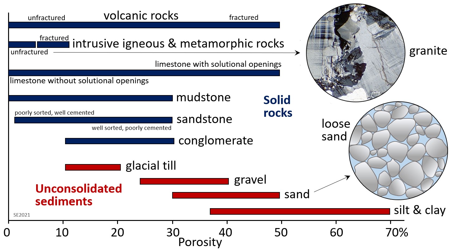
Consolidation and cementation during the process of lithification of sediments into sedimentary rocks reduces primary porosity. Sedimentary rocks generally have porosities in the range of 10% to 25%, some of which may be secondary (fracture) porosity. The grain size, sorting, compaction, and degree of cementation of the rocks all influence primary porosity. For example, poorly sorted and well-cemented sandstone and well-compressed mudstone can have low porosity. Igneous or metamorphic rocks have the lowest primary porosity because they commonly form at depth and their crystals are interlocking. Most of their porosity is secondary porosity in fractures. Of the consolidated rocks, well-fractured volcanic rocks and limestone that has cavernous openings produced by dissolution have the highest potential porosity, while intrusive igneous and metamorphic rocks, which formed under great pressure, have the lowest.

Porosity is a measure of how much water can be stored in geological materials. Almost all rocks have some porosity and therefore contain groundwater. Groundwater is present under your feet and everywhere on the planet. Considering that sedimentary rocks and unconsolidated sediments cover about 75% of the continental crust with an average thickness of a few hundred metres, and that they are likely to have around 20% porosity on average, it is easy to see that a huge volume of water is stored in the ground.

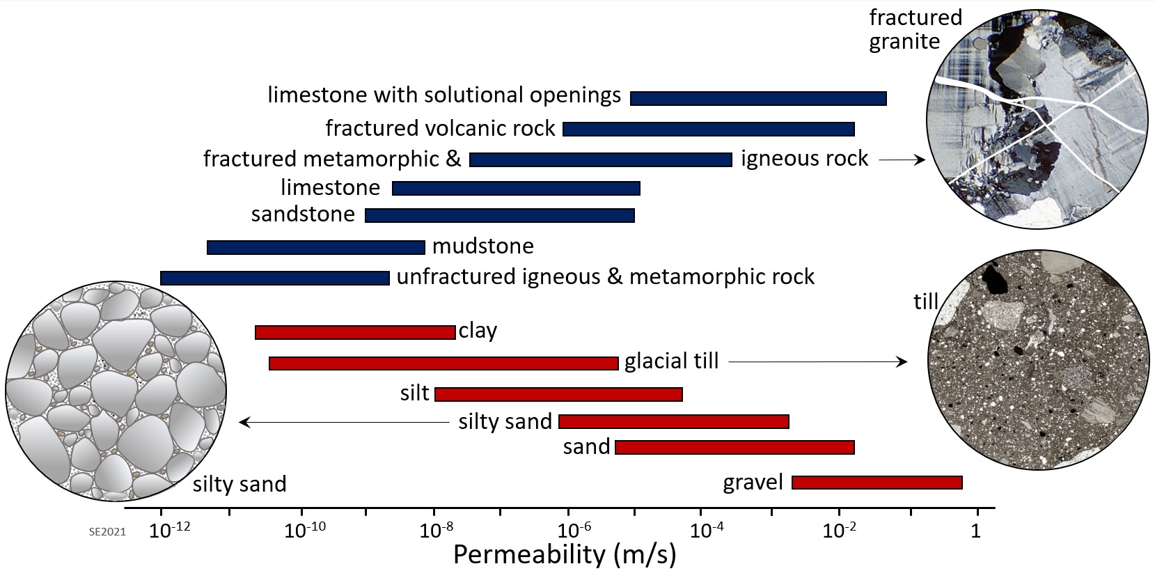
While porosity is a measure of open space, permeability is related to the sizes of those spaces and how they are shaped and interconnected, and so determines how easy it is for water to flow through the material. Larger pores mean there is less friction between flowing water and the sides of the pores. Smaller pores mean more friction along pore walls, and also more twists and turns for the water to have to flow-through. Permeability controls how quickly water can flow through the rock or unconsolidated sediment and how easy it will be to extract the water for our purposes. Permeability is the most important variable in controlling groundwater flow rate and the quality of an aquifer as a source of water. Permeability can be expressed in a range of different units; in this book we will use metres per second, which is also termed the hydraulic conductivity (K, m/s).

As shown on Figure 11.4.2 there is a wide range of permeabilities in geological materials from hydraulic conductivities of 10⁻¹² metres per second (0.000000000001 m/s) to approaching 1 m/s. Unconsolidated materials are generally more permeable than the corresponding rocks (compare sand with sandstone, for example), and the coarser materials are generally more permeable than the finer ones. The least permeable rocks are unfractured intrusive igneous and metamorphic rocks, followed by unfractured mudstone, sandstone, and limestone. The permeability of sandstone can vary widely depending on the rock’s degree of sorting and cementation. Volcanic rocks can be highly permeable—especially if they are fractured—as can limestone that has been dissolved along fractures and bedding planes to create solutional openings.

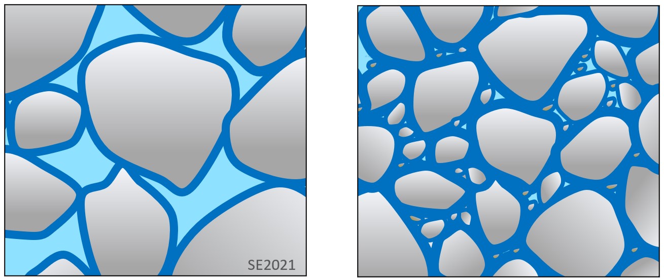
Grain size is critically important to permeability because it influences the extent to which the water adheres to the grains and so is reluctant to flow. A molecule of water (H₂O) is polar, in that it is positively charged near the two hydrogen atoms, and negatively charged near the oxygen atom. The outer surface of most silicate minerals has a slight negative ionic charge, which creates adhesive forces between mineral surfaces and the positive sides of water molecules. Water adhesion to grains is only effective for a short distance away from a surface. This is illustrated on Figure 11.4.3, where dark blue represents water that is held to surfaces by adhesion and light blue is water that is more free to move. If the grains are large (sand-sized) and therefore the pores are large, most of the water in the pores is not affected by adhesion (left side) and is free to move. If the grains are small (silt- and clay-sized) and the pores are small, more of the water will be near to a grain surface, and thus will held in place by adhesion (right side), and therefore less able to move, making the material less permeable.

Surface water and groundwater are both active parts of the hydrologic cycle that moves water from where it has been deposited on the land surface as rain or snow, back to the ocean. The water within a watershed is all linked.

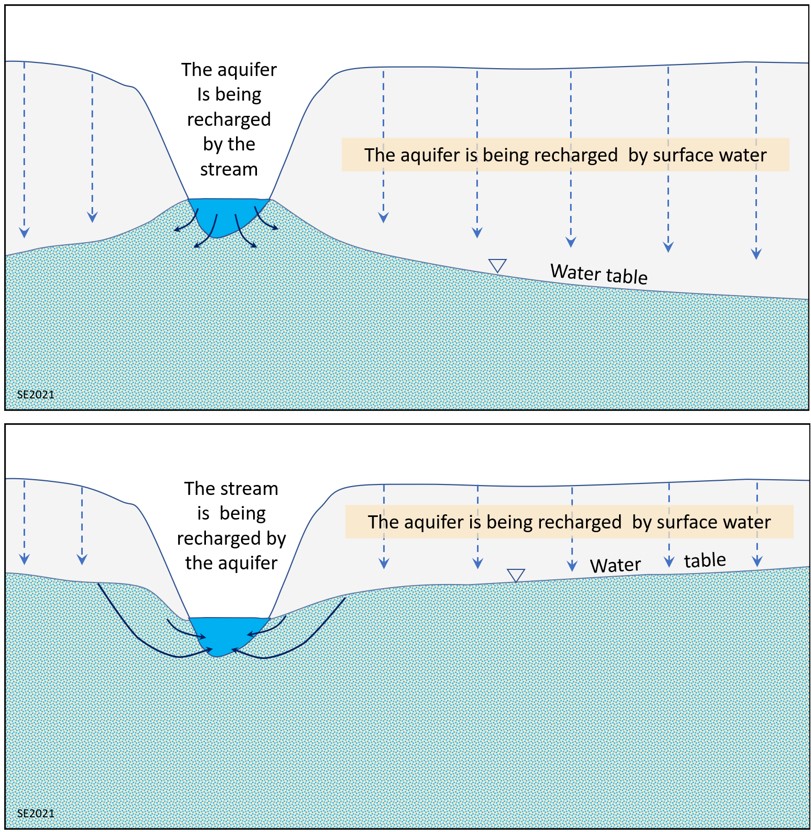
There is ongoing exchange of water between surface water (streams, lakes etc.) and the groundwater. One aspect of this exchange is illustrated on Figure 11.4.4 (top), which shows how an unconfined aquifer may be recharged by water from a stream, and also by water percolating downward from surface. The aquifer shown here is partly saturated with water, and the upper limit of the zone of saturation is known as the water table. The water table intersects the surface where there is a stream or a lake.

At a different time of year, when the water table is higher, water may flow from the aquifer into the stream, supplementing the stream flow (Figure 11.4.4, bottom). See Box 11.1 below for an illustration of the importance of the contribution of groundwater to stream flow.

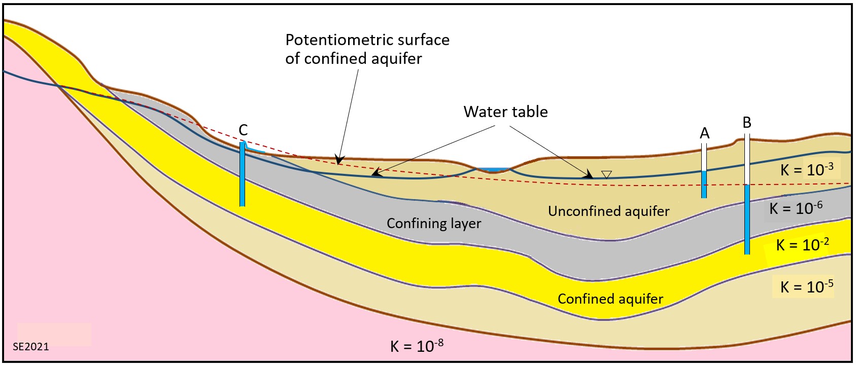
The porosities and permeabilities of different geological materials help us to define their water storage and water supply capabilities so that we can identify which materials might be useful as a groundwater source, and which might not. An aquifer is a body of sediment or rock that has sufficiently high permeability that we can easily extract water for our use using a well. An aquitard (or confining layer) is a body that has too little permeability to be useful. This concept is illustrated on Figure 11.4.5 which shows an aquifer at the top (labelled “Unconfined aquifer”). The level of the water in well A is at the same height as the water table at that location.

The unconfined aquifer is underlain by a layer of relatively impermeable material, here labelled a “Confining layer” which could also be called an aquitard. This is underlain by another permeable layer which is labelled as a “Confined aquifer”. Water can enter the confined aquifer only in the area where it is exposed (upper left) and because that is at a relatively high elevation the groundwater at depth in this aquifer is under pressure. The red-dashed line defines the pressure at any point in this aquifer, and that is equivalent to the height to which water would rise in a well at that location. This is called the potentiometric surface. A well drilled at B is known as artesian because the water rises above the upper surface of the confined aquifer. The well at C is also artesian, but because the potentiometric surface is above the ground surface at that location this is a flowing artesian well. There could be more than one confined aquifer in a region. In that case, each would have its own potentiometric surface.

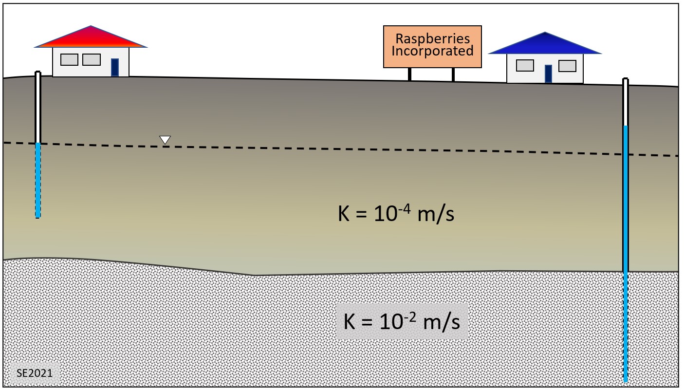
It is important to note that the distinction between an aquifer and an aquitard is subjective. As shown on Figure 11.4.6, a groundwater user with only a modest need for water may consider a body with low permeability to be an aquifer, while someone with a need for a lot of water might consider that same body to be an aquitard.

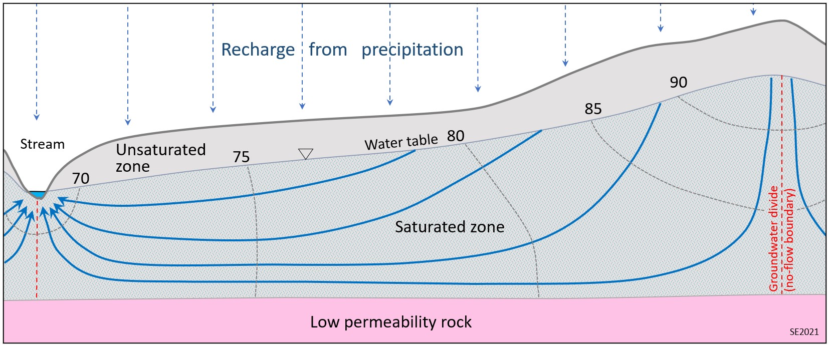
Groundwater flows from areas of high hydraulic head (high water table or potentiometric surface) to areas of lower hydraulic head. This is shown on Figure 11.4.7, which also illustrates the concept of a groundwater divide (red-dashed lines), where the slope of the water table changes directions. Precipitation on the ground surface leads to recharge of the groundwater system. Water doesn’t flow across a groundwater divide, which is why it is also termed a no-flow boundary. Groundwater flow lines always cross hydraulic head contour lines (also known as equipotential lines) at right angles.

In 1856, French engineer Henri Darcy derived a method for estimating the volume of groundwater flow based on the hydraulic gradient and the permeability of an aquifer. Darcy’s equation, which has been used widely by hydrogeologists ever since, looks like this:

Q = K × i ×A

where Q is the volume of the groundwater flow (m³/s), K is the permeability (m/s), i is the hydraulic gradient, and A is the cross-sectional area of the aquifer perpendicular to the flow.

The following equation can be used to determine the flux (i.e., volume per unit time per unit area of aquifer) of groundwater passing through the area of the aquifer being considered. This is how much groundwater flows through each unit area of aquifer:

q = Q/A = K × i

Lower-case q is known as the Darcy flux; it typically has units of metres per second (although other units can be used, such as cm/day or ft/minute). It is not the velocity of the groundwater, but is an estimate of how much volume (m³/s) passes through each area (m²), so the typical units are (m³/s)/m², which is shortened to m/s. In reality, the groundwater does not pass through all of the cross-sectional area of the aquifer (A); it can only pass through the pores. The actual velocity of the water is the rate at which the water must move through the pores in order to get the same flux through the actual open area (total area × porosity). So, the equation to estimate flow velocity is as follows:

V = (K × i)/n

where V is the velocity of the groundwater in m/s, and n is the porosity (expressed as a proportion, so if the porosity is 10%, n = 0.1).

We can apply this equation to the scenario in Figure 11.4.8 to estimate the groundwater velocity. The hydraulic gradient (i) is the difference in elevation of the water table at two points in the aquifer, divided by the distance between those two points. The elevation of the water table at the well is 90 m and that at the stream is 70 m. The two points are 250 m apart, so i = (90-70m )/250 m= 0.08. The hydraulic gradient expresses m of head change per m of distance or m/m, which means it has no units. If the permeability is 0.00001 metres per second (m/s), and if the material has a porosity of 25%, then the velocity of the groundwater can be estimated using:

V = (0.00001 m/s x 0.08)/0.25 = 0.0000032 m/s

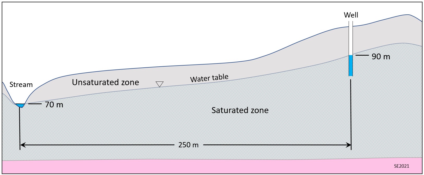
That is equivalent to 0.000192 metres/minute, 0.0115 metres/hour or 0.276 m/day. That means that, in this example, it would take 361 days for water to travel the 250 metres from the vicinity of the well to the stream. Groundwater moves slowly, and that is a reasonable amount of time for water to move that distance. In fact, it would likely take a little longer than that, because, as we’ve seen from Figure 11.4.7, it doesn’t travel in a straight line.

Exercise 11.3 Groundwater Flow Rate

Joe’s Gas station has an underground storage tank (UST) that is corroded and is leaking fuel into the aquifer.  Joe is concerned that any components of the fuel that mix with groundwater could contaminate a nearby stream and wants to find out how quickly that could happen. The scenario is illustrated on Figure 11.4.9. The water level in the well next to the gas station is 37 m above sea level, while the stream, 80 m away, is at 21 m. Assume that the aquifer has a permeability of 0.0002 m/s and a porosity of 15%.

Use the equation V = (K × i)/n to estimate the flow rate of water in the aquifer in the direction from the gas station to the stream. Use that number to determine how long it is likely to take the contaminated groundwater to reach the stream.

Exercise answers are provided Appendix 2.

It is critical to understand that—except in limestone karst regions—groundwater does not flow in underground streams, nor does it form underground lakes. In almost all cases, groundwater flows very slowly through the pores in granular sediments, or through the fractures in solid rock. Flow velocities of several centimetres per day are possible in permeable sediments with significant hydraulic gradients. But in many cases, permeabilities are lower than the ones used in the examples above, and gradients are much lower. It is not uncommon for groundwater to flow at velocities of a few centimetres per year, or even just a few millimetres per year.

Box 11.3 Nile Creek Surface Water and Groundwater

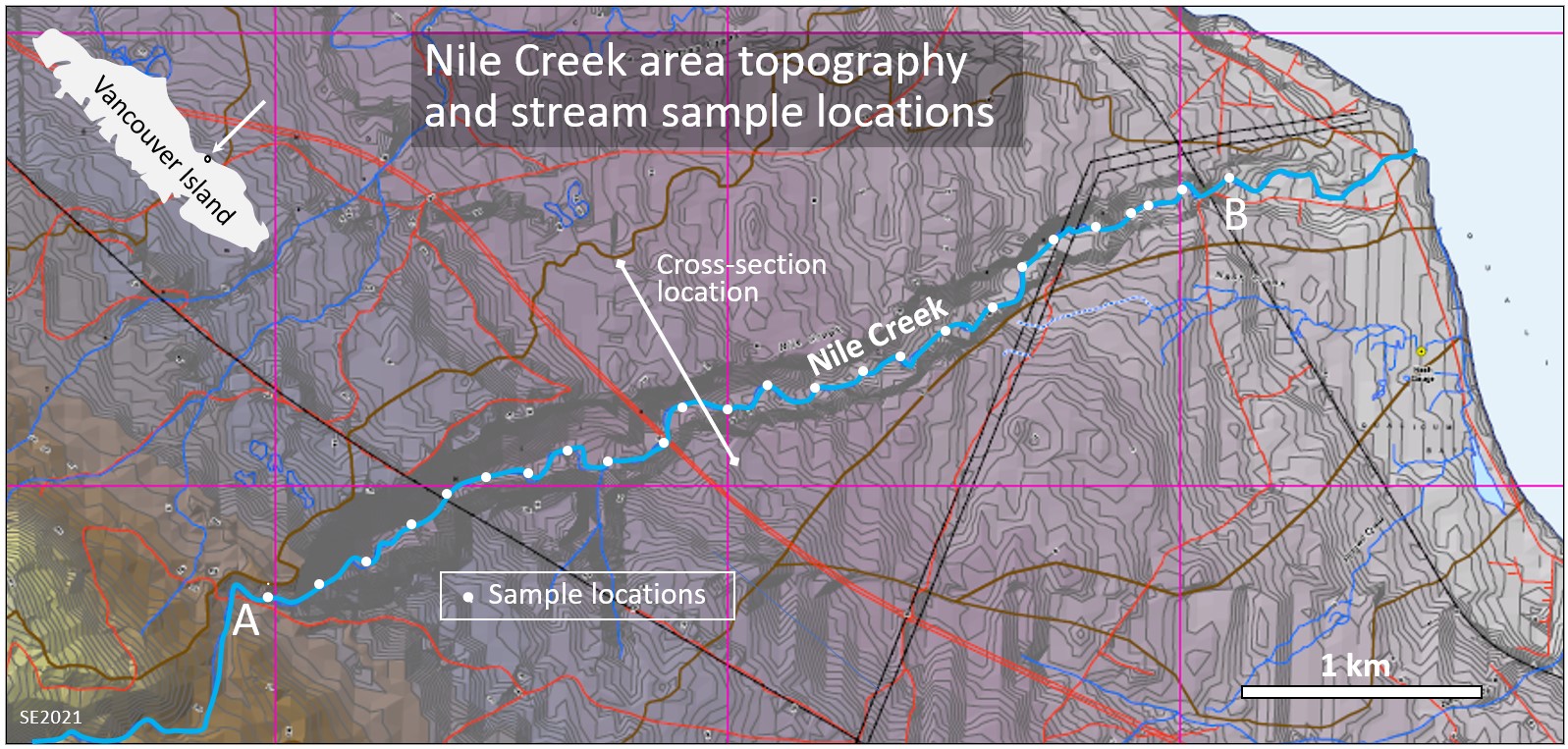
Nile Creek is a small stream on the east side of Vancouver Island (Figure 11.4.10). It has strong year-round flow and supports a significant population of pink salmon (Oncorhynchus gorbuscha).

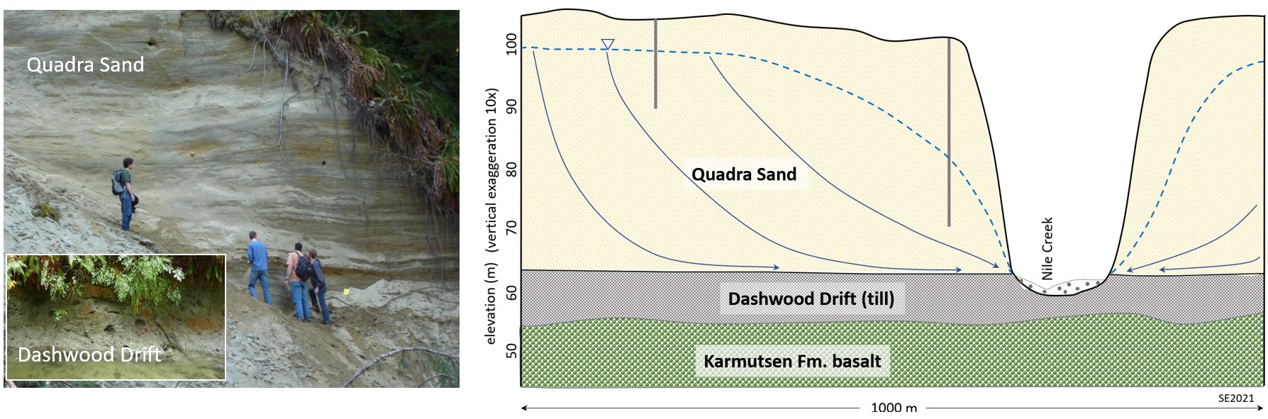
The Nile Creek valley is incised into a 50 m thick deposit of glacial outwash sand (Quadra Sand) that is underlain by till (Dashwood Drift) which is underlain by basaltic rock (Karmutsen Fm) (Figure 11.4.11). The Quadra Sand is quite permeable while the Dashwood drift is much less permeable.

In 2011 and 2012 Trout Unlimited Canada sponsored a project to improve our understanding of why Nile Creek provides good habitat for Pink Salmon (https://tucanada.org/nile-creek/). Water samples were taken at numerous locations along the stream, at different times of the year, and analyzed for a range of parameters, including pH, conductivity (which is a measure of the total amount of dissolved solids) and temperature.

Results for conductivity and temperature in September 2012 are shown on Figure 11.4.12. Point A is where the stream emerges from an upland area underlain only by Karmutsen Fm. basalt and enters the deeply incised valley. About 500 m downstream from that point the temperature of the water decreased sharply from around 14° C to about 9° C, while the conductivity increased from around 60 µs/cm to over 75 µs/cm. Similar data from six months earlier (February 2011) shows a comparable increase in conductivity, but in February the very cold stream water becomes warmer rather than colder as it flows through the deep valley.

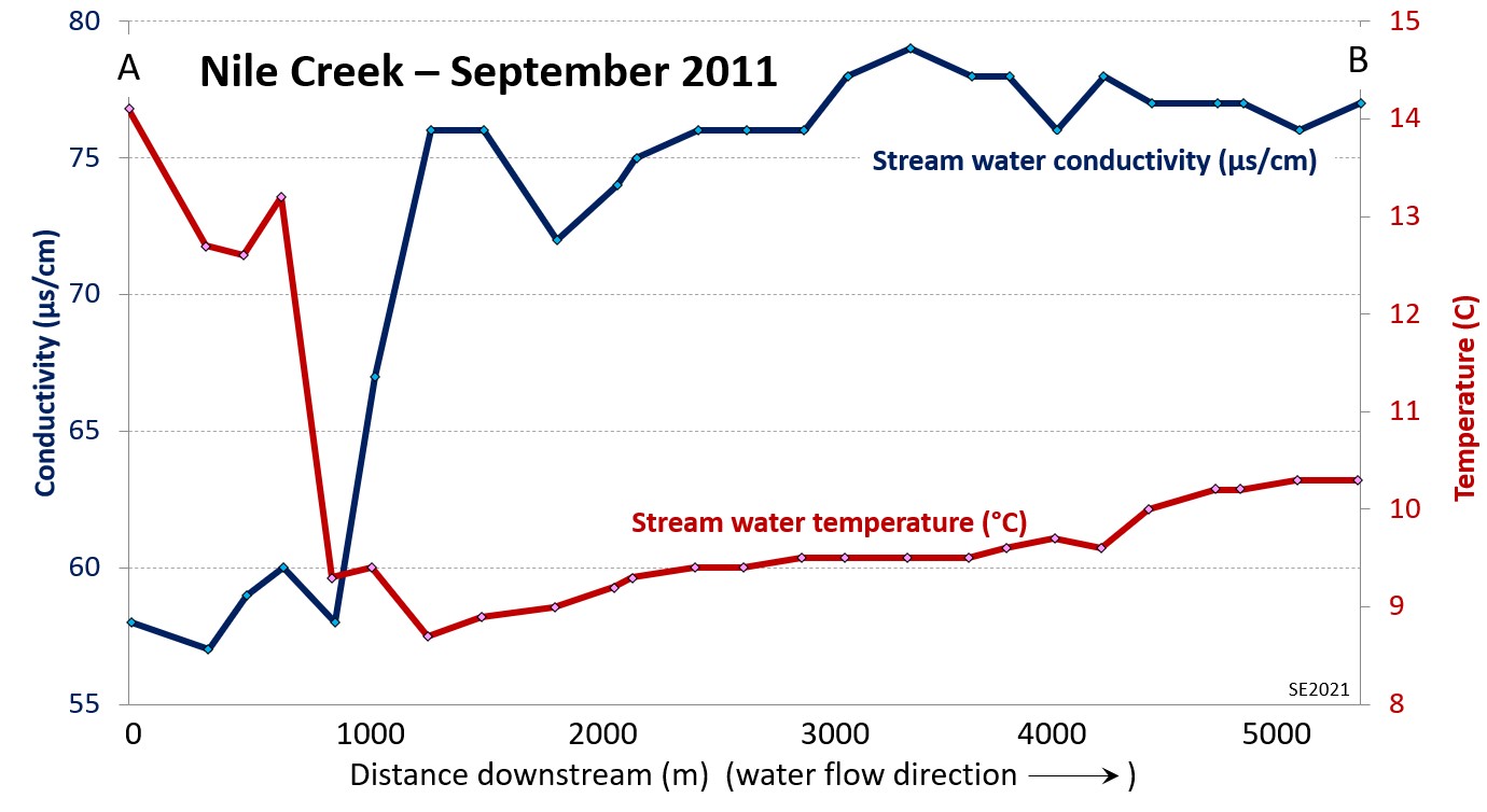
The implication of these observed changes is that there is a significant contribution of groundwater to the flow of Nile Creek within the incised section. That groundwater has a higher conductivity (in the order of 100 µs/cm) than the surface water, and at around 10° C it is cooler than the surface water in summer, and warmer than the surface water in the winter. Based on available information on the conductivity and temperature of the groundwater in the Quadra Sand it is estimated that 70 to 90% of the summertime flow of Nile Creek is derived from groundwater coming from the Quadra Sand aquifer. In winter, when the surface flow is always much higher, 20 to 30% of the flow is from groundwater. The significant contribution of groundwater to the flow of Nile Creek is key to its success as a salmon stream. An important corollary is that in order to ensure that streams like this continue to provide habitat for fish and other organisms we also need to protect the surrounding aquifers.

Exercise 11.4 Cone of Depression

When a well is pumped at a rate that is faster than rate at which water can flow into it (as governed by the permeability of the aquifer) the water level in the well will drop and a cone of depression will develop around the well. This is illustrated for well A in Figure 11.4.13. (Wells B and C are not being pumped at this time.)

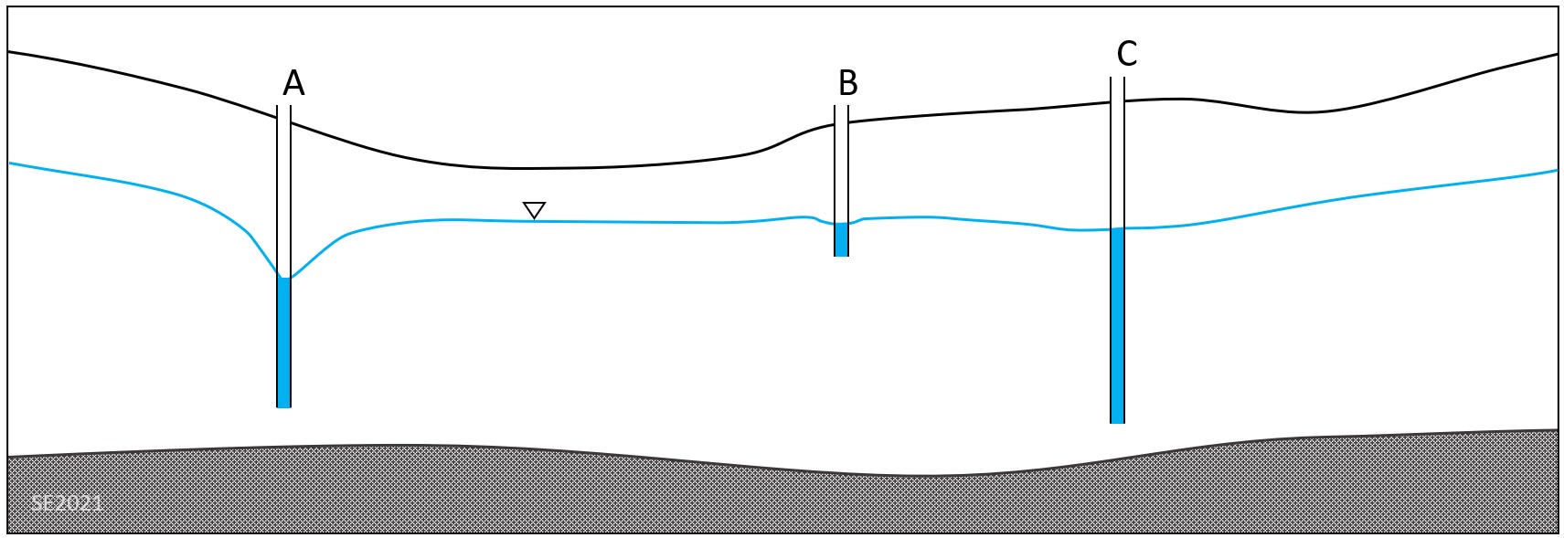
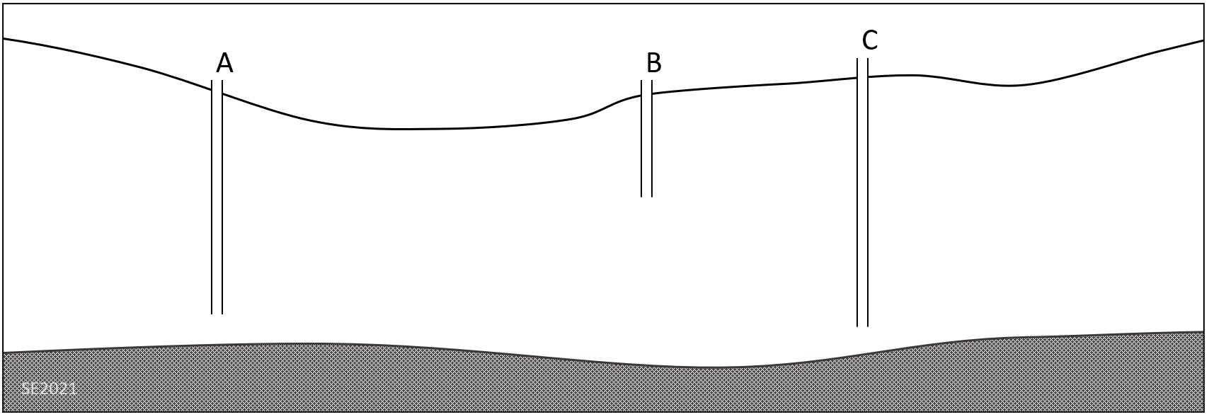
Using Figure 11.4.14 draw the water table to show what would happen if well C was pumped fast enough to create a cone of depression that resulted in well B going dry.

Exercise answers are provided Appendix 2.

Groundwater is the basis for water movement in a drainage basin. Literally, the base. Any water that cannot flow out of the drainage basin while still under the ground will end up flowing into low spots on the landscape, contributing to the flow in streams and lakes. Those flows are supplemented by surface runoff.

What we need to recognize is that pumping any amount of groundwater takes away from surface water somewhere in the drainage basin (unless we later rehabilitate that water and return it to the environment). It’s OK to use groundwater, but we need to recognize that groundwater and surface water are really all the same thing, and so we need to be careful not to use so much that we negatively affect other users, including ecosystems.

Media Attributions

• Figure 11.4.1 Steven Earle, CC BY 4.0
• Figure 11.4.2 Steven Earle, CC BY 4.0
• Figure 11.4.3 Steven Earle, CC BY 4.0
• Figure 11.4.4 Steven Earle, CC BY 4.0
• Figure 11.4.5 Steven Earle, CC BY 4.0
• Figure 11.4.6 Steven Earle, CC BY 4.0
• Figure 11.4.7 Steven Earle, CC BY 4.0
• Figure 11.4.8 Steven Earle, CC BY 4.0
• Figure 11.4.9 Steven Earle, CC BY 4.0
• Figure 11.4.10 Steven Earle, CC BY 4.0, after Trout Unlimited Canada, https://tucanada.org/
• Figure 11.4.11 Steven Earle, CC BY 4.0
• Figure 11.4.12 Steven Earle, CC BY 4.0
• Figure 11.4.13 Steven Earle, CC BY 4.0
• Figure 11.4.14 Steven Earle, CC BY 4.0

Reference

Nile Creek-Qualicum Bay restoration and enhancement: Reconnecting coastal cutthroat trout and salmon to their habitat. (2011). Trout Unlimited Canada. https://tucanada.org/project/nile-creek-qualicum-bay-restoration-and-enhancement/