<?xml version="1.0" encoding="UTF-8"?>
<!DOCTYPE html PUBLIC "-//W3C//DTD XHTML 1.1//EN" "http://www.w3.org/TR/xhtml11/DTD/xhtml11.dtd">
<html xmlns="http://www.w3.org/1999/xhtml" xml:lang="en">
<head>
<meta content="text/html; charset=UTF-8" http-equiv="content-type" />
<meta http-equiv="Content-Language" content="en" />
<meta name="generator" content="Pressbooks 6.19.0" />
<meta name="pb-authors" content="Steve Earle" />
<meta name="pb-title" content="Environmental Geology" />
<meta name="pb-language" content="en-ca" />
<meta name="pb-cover-image" content="https://environmental-geol.pressbooks.tru.ca/wp-content/uploads/sites/123/2022/11/environmental_geology_cover_online.png" />
<meta name="pb-book-license" content="cc-by-nc-sa" />
<meta name="pb-publisher" content="TRU Open Learning" />
<meta name="pb-publisher-city" content="Kamloops" />
<meta name="pb-primary-subject" content="R" />
<meta name="pb-copyright-holder" content="Steve Earle, Thompson Rivers University" />
<meta name="pb-about-50" content="Environmental Geology is a college-level textbook exploring Earth systems, climate change, natural hazards, and vital resources. With rich illustrations and interactive exercises, it engages students in key geological processes and their environmental impacts." />
<meta name="pb-about-unlimited" content="Environmental Geology is a comprehensive, up-to-date textbook for college-level courses on the environmental aspects of Earth Science. It covers Earth systems, climate change, glaciation, natural hazards like earthquakes and floods, and essential resources such as water, energy, and metals. Richly illustrated with embedded exercises—some interactive—it engages students as they explore key geological processes and their environmental impacts." />
<meta name="pb-custom-copyright" content="© 2021 Steven Earl, Thompson Rivers UniversityEnvironmental Geology by Steven Earle is licensed under a  CC BY-NC-SA 4.0 licence." />
<meta name="pb-publication-date" content="1638316800" />
<meta name="pb-additional-subjects" content="RB, RNFY, RNPG, RNR, YPMP7" />
<title>Environmental Geology</title>
</head>
<body lang='en' >
<div id="half-title-page"><h1 class="title">Environmental Geology</h1></div>
<div id="title-page">
			<h1 class="title">Environmental Geology</h1>
		<h2 class="subtitle"></h2>
					<p class="author">Steve Earle</p>
								<p class="publisher">TRU Open Learning</p>
		<p class="publisher-city">Kamloops</p>
	</div>
<div id="copyright-page">
	<div class="ugc">
					
<div class="license-attribution"><p><img src="https://environmental-geol.pressbooks.tru.ca/wp-content/themes/pressbooks-book/packages/buckram/assets/images/cc-by-nc-sa.svg" alt="Icon for the Creative Commons Attribution-NonCommercial-ShareAlike 4.0 International License" /></p><p>Environmental Geology Copyright © 2021 by <span>Steve Earle, Thompson Rivers University</span> is licensed under a <a rel="license" href="https://creativecommons.org/licenses/by-nc-sa/4.0/">Creative Commons Attribution-NonCommercial-ShareAlike 4.0 International License</a>, except where otherwise noted.</p></div>

							<p>© 2021 Steven Earl, Thompson Rivers University</p><p><i><a href="https://trucareertext.pressbooks.tru.ca/">Environmental Geology</a></i> by Steven Earle is licensed under a  <a href="https://creativecommons.org/licenses/by-nc-sa/4.0/">CC BY-NC-SA 4.0 licence</a>.</p>
							</div>
</div>
<div id="toc">
	<h1>Contents</h1>
	<ul>
					<li class="front-matter miscellaneous">
	<a href="#front-matter-introduction">
		<span class="toc-chapter-title">Introduction</span>
							</a>
	</li>

					<li class="part">
	<a href="#part-chapter-1-earth-system-science-and-environmental-geology">
					Chapter 1 Earth System Science and Environmental Geology
			</a>
</li>

					<li class="chapter standard">
	<a href="#chapter-the-earth-in-space">
		<span class="toc-chapter-title">1.1 The Earth in Space</span>
							<span class="chapter-author">Steve Earle</span>
					</a>
	</li>

					<li class="chapter standard">
	<a href="#chapter-earth-system-science">
		<span class="toc-chapter-title">1.2 Earth System Science</span>
							<span class="chapter-author">Steve Earle</span>
					</a>
	</li>

					<li class="chapter standard">
	<a href="#chapter-environmental-geology">
		<span class="toc-chapter-title">1.3 Environmental Geology</span>
							<span class="chapter-author">Steve Earle</span>
					</a>
	</li>

					<li class="chapter standard">
	<a href="#chapter-chapter-1-summary">
		<span class="toc-chapter-title">Chapter 1 Summary and Questions for Review</span>
							<span class="chapter-author">Steve Earle</span>
					</a>
	</li>

					<li class="part">
	<a href="#part-chapter-2-review-of-physical-geology">
					Chapter 2 Review of Physical Geology
			</a>
</li>

					<li class="chapter standard">
	<a href="#chapter-minerals">
		<span class="toc-chapter-title">2.1 Minerals </span>
							<span class="chapter-author">Steve Earle</span>
					</a>
	</li>

					<li class="chapter standard">
	<a href="#chapter-rocks">
		<span class="toc-chapter-title">2.2 Rocks</span>
							<span class="chapter-author">Steve Earle</span>
					</a>
	</li>

					<li class="chapter standard">
	<a href="#chapter-earths-interior">
		<span class="toc-chapter-title">2.3 Earth’s Interior</span>
							<span class="chapter-author">Steve Earle</span>
					</a>
	</li>

					<li class="chapter standard">
	<a href="#chapter-plate-tectonics">
		<span class="toc-chapter-title">2.4 Plate Tectonics</span>
							<span class="chapter-author">Steve Earle</span>
					</a>
	</li>

					<li class="chapter standard">
	<a href="#chapter-geosphere-earth-systems">
		<span class="toc-chapter-title">2.5 Geosphere Earth Systems</span>
							<span class="chapter-author">Steve Earle</span>
					</a>
	</li>

					<li class="chapter standard">
	<a href="#chapter-summary-and-questions-for-review">
		<span class="toc-chapter-title">Chapter 2 Summary and Questions for Review</span>
							<span class="chapter-author">Steve Earle</span>
					</a>
	</li>

					<li class="part">
	<a href="#part-chapter-3-climate-changes-in-earths-past">
					Chapter 3 Climate Changes in Earth’s Past
			</a>
</li>

					<li class="chapter standard">
	<a href="#chapter-changes-in-solar-output-and-in-the-earths-atmosphere">
		<span class="toc-chapter-title">3.1 Changes in Solar Output and in the Earth’s Atmosphere</span>
							<span class="chapter-author">Steve Earle</span>
					</a>
	</li>

					<li class="chapter standard">
	<a href="#chapter-plate-tectonics-and-climate-change">
		<span class="toc-chapter-title">3.2 Plate Tectonics and Climate Change</span>
							<span class="chapter-author">Steve Earle</span>
					</a>
	</li>

					<li class="chapter standard">
	<a href="#chapter-volcanism-and-climate-change">
		<span class="toc-chapter-title">3.3 Volcanism and Climate Change</span>
							<span class="chapter-author">Steve Earle</span>
					</a>
	</li>

					<li class="chapter standard">
	<a href="#chapter-earths-orbital-fluctuations-and-climate-change">
		<span class="toc-chapter-title">3.4 Earth’s Orbital Fluctuations and Climate Change</span>
							<span class="chapter-author">Steve Earle</span>
					</a>
	</li>

					<li class="chapter standard">
	<a href="#chapter-ocean-currents-and-climate-change">
		<span class="toc-chapter-title">3.5 Ocean Currents and Climate Change</span>
							<span class="chapter-author">Steve Earle</span>
					</a>
	</li>

					<li class="chapter standard">
	<a href="#chapter-extraterrestrial-impacts-and-climate-change">
		<span class="toc-chapter-title">3.6 Extraterrestrial Impacts and Climate Change</span>
							<span class="chapter-author">Steve Earle</span>
					</a>
	</li>

					<li class="chapter standard">
	<a href="#chapter-summary-and-questions-for-review-2">
		<span class="toc-chapter-title">Chapter 3 Summary and Questions for Review</span>
							<span class="chapter-author">Steve Earle</span>
					</a>
	</li>

					<li class="part">
	<a href="#part-chapter-4-glaciation">
					Chapter 4 Glaciation
			</a>
</li>

					<li class="chapter standard">
	<a href="#chapter-glacial-periods-in-earths-history">
		<span class="toc-chapter-title">4.1 Glacial Periods in Earth’s History</span>
							<span class="chapter-author">Steve Earle</span>
					</a>
	</li>

					<li class="chapter standard">
	<a href="#chapter-how-glaciers-work">
		<span class="toc-chapter-title">4.2 How Glaciers Work</span>
							<span class="chapter-author">Steve Earle</span>
					</a>
	</li>

					<li class="chapter standard">
	<a href="#chapter-glacial-erosion">
		<span class="toc-chapter-title">4.3 Glacial Erosion</span>
							<span class="chapter-author">Steve Earle</span>
					</a>
	</li>

					<li class="chapter standard">
	<a href="#chapter-glacial-deposits">
		<span class="toc-chapter-title">4.4 Glacial Deposits</span>
							<span class="chapter-author">Steve Earle</span>
					</a>
	</li>

					<li class="chapter standard">
	<a href="#chapter-glaciers-and-climate-change-glaciers-and-earth-systems">
		<span class="toc-chapter-title">4.5 Glaciers and Climate Change, Glaciers and Earth Systems</span>
							<span class="chapter-author">Steve Earle</span>
					</a>
	</li>

					<li class="chapter standard">
	<a href="#chapter-slug-279-2">
		<span class="toc-chapter-title">Chapter 4 Summary and Questions for Review</span>
							<span class="chapter-author">Steve Earle</span>
					</a>
	</li>

					<li class="part">
	<a href="#part-chapter-5-mass-wasting">
					Chapter 5 Mass Wasting
			</a>
</li>

					<li class="chapter standard">
	<a href="#chapter-factors-that-control-slope-stability">
		<span class="toc-chapter-title">5.1 Factors that Control Slope Stability</span>
							<span class="chapter-author">Steve Earle</span>
					</a>
	</li>

					<li class="chapter standard">
	<a href="#chapter-classification-of-mass-wasting">
		<span class="toc-chapter-title">5.2 Classification of Mass Wasting </span>
							<span class="chapter-author">Steve Earle</span>
					</a>
	</li>

					<li class="chapter standard">
	<a href="#chapter-mitigating-the-effects-of-mass-wasting">
		<span class="toc-chapter-title">5.3 Mitigating the Effects of Mass Wasting</span>
							<span class="chapter-author">Steve Earle</span>
					</a>
	</li>

					<li class="chapter standard">
	<a href="#chapter-mass-wasting-and-earth-systems">
		<span class="toc-chapter-title">5.4 Mass Wasting and Earth Systems</span>
							<span class="chapter-author">Steve Earle</span>
					</a>
	</li>

					<li class="chapter standard">
	<a href="#chapter-chapter-5-summary-and-questions-for-review">
		<span class="toc-chapter-title">Chapter 5 Summary and Questions for Review</span>
							<span class="chapter-author">Steve Earle</span>
					</a>
	</li>

					<li class="part">
	<a href="#part-chapter-6-earthquakes">
					Chapter 6 Earthquakes
			</a>
</li>

					<li class="chapter standard">
	<a href="#chapter-what-is-an-earthquake">
		<span class="toc-chapter-title">6.1 What is an Earthquake?</span>
							<span class="chapter-author">Steve Earle</span>
					</a>
	</li>

					<li class="chapter standard">
	<a href="#chapter-earthquakes-and-plate-tectonics">
		<span class="toc-chapter-title">6.2 Earthquakes and Plate Tectonics</span>
							<span class="chapter-author">Steve Earle</span>
					</a>
	</li>

					<li class="chapter standard">
	<a href="#chapter-measuring-earthquakes">
		<span class="toc-chapter-title">6.3 Measuring Earthquakes</span>
							<span class="chapter-author">Steve Earle</span>
					</a>
	</li>

					<li class="chapter standard">
	<a href="#chapter-the-impacts-of-earthquakes">
		<span class="toc-chapter-title">6.4 The Impacts of Earthquakes</span>
							<span class="chapter-author">Steve Earle</span>
					</a>
	</li>

					<li class="chapter standard">
	<a href="#chapter-forecasting-earthquakes-and-minimizing-damage-and-casualties">
		<span class="toc-chapter-title">6.5 Forecasting Earthquakes and Minimizing Damage and Casualties</span>
							<span class="chapter-author">Steve Earle</span>
					</a>
	</li>

					<li class="chapter standard">
	<a href="#chapter-chapter-6-summary-and-questions-for-review">
		<span class="toc-chapter-title">Chapter 6 Summary and Questions for Review</span>
							<span class="chapter-author">Steve Earle</span>
					</a>
	</li>

					<li class="part">
	<a href="#part-chapter-7-volcanism">
					Chapter 7 Volcanism
			</a>
</li>

					<li class="chapter standard">
	<a href="#chapter-plate-tectonic-settings-of-volcanism">
		<span class="toc-chapter-title">7.1 Plate Tectonic Settings of Volcanism</span>
							<span class="chapter-author">Steve Earle</span>
					</a>
	</li>

					<li class="chapter standard">
	<a href="#chapter-magma-composition-and-eruption-style">
		<span class="toc-chapter-title">7.2 Magma Composition and Eruption Style</span>
							<span class="chapter-author">Steve Earle</span>
					</a>
	</li>

					<li class="chapter standard">
	<a href="#chapter-types-of-volcanism">
		<span class="toc-chapter-title">7.3 Types of Volcanism</span>
							<span class="chapter-author">Steve Earle</span>
					</a>
	</li>

					<li class="chapter standard">
	<a href="#chapter-volcanic-hazards">
		<span class="toc-chapter-title">7.4 Volcanic Hazards</span>
							<span class="chapter-author">Steve Earle</span>
					</a>
	</li>

					<li class="chapter standard">
	<a href="#chapter-monitoring-volcanoes-and-predicting-eruptions">
		<span class="toc-chapter-title">7.5 Monitoring Volcanoes and Predicting Eruptions</span>
							<span class="chapter-author">Steve Earle</span>
					</a>
	</li>

					<li class="chapter standard">
	<a href="#chapter-effects-of-volcanic-eruptions-on-humans-and-on-earth-systems">
		<span class="toc-chapter-title">7.6 Effects of Volcanic Eruptions on Humans and on Earth Systems</span>
							<span class="chapter-author">Steve Earle</span>
					</a>
	</li>

					<li class="chapter standard">
	<a href="#chapter-chapter-7-summary-and-questions-for-review">
		<span class="toc-chapter-title">Chapter 7 Summary and Questions for Review</span>
							<span class="chapter-author">Steve Earle</span>
					</a>
	</li>

					<li class="part">
	<a href="#part-chapter-8-geological-resources">
					Chapter 8 Geological Resources
			</a>
</li>

					<li class="chapter standard">
	<a href="#chapter-metal-deposits">
		<span class="toc-chapter-title">8.1 Metal Deposits</span>
							<span class="chapter-author">Steve Earle</span>
					</a>
	</li>

					<li class="chapter standard">
	<a href="#chapter-mining-and-ore-processing">
		<span class="toc-chapter-title">8.2 Mining and Ore Processing </span>
							<span class="chapter-author">Steve Earle</span>
					</a>
	</li>

					<li class="chapter standard">
	<a href="#chapter-industrial-minerals">
		<span class="toc-chapter-title">8.3 Industrial Minerals </span>
							<span class="chapter-author">Steve Earle</span>
					</a>
	</li>

					<li class="chapter standard">
	<a href="#chapter-fossil-fuels">
		<span class="toc-chapter-title">8.4 Fossil Fuels</span>
							<span class="chapter-author">Steve Earle</span>
					</a>
	</li>

					<li class="chapter standard">
	<a href="#chapter-the-implications-of-resource-extraction-for-the-climate-and-earth-systems">
		<span class="toc-chapter-title">8.5 The Implications of Resource Extraction for the Climate and Earth Systems</span>
							<span class="chapter-author">Steve Earle</span>
					</a>
	</li>

					<li class="chapter standard">
	<a href="#chapter-chapter-8-summary-and-questions-for-review">
		<span class="toc-chapter-title">Chapter 8 Summary and Questions for Review</span>
							<span class="chapter-author">Steve Earle</span>
					</a>
	</li>

					<li class="part">
	<a href="#part-chapter-9-energy-resources">
					Chapter 9 Energy Resources
			</a>
</li>

					<li class="chapter standard">
	<a href="#chapter-solar-and-wind">
		<span class="toc-chapter-title">9.1 Solar and Wind</span>
							<span class="chapter-author">Steve Earle</span>
					</a>
	</li>

					<li class="chapter standard">
	<a href="#chapter-hydro">
		<span class="toc-chapter-title">9.2 Hydro</span>
							<span class="chapter-author">Steve Earle</span>
					</a>
	</li>

					<li class="chapter standard">
	<a href="#chapter-wave-and-tidal-energy">
		<span class="toc-chapter-title">9.3 Wave and Tidal Energy</span>
							<span class="chapter-author">Steve Earle</span>
					</a>
	</li>

					<li class="chapter standard">
	<a href="#chapter-geothermal-and-geo-exchange">
		<span class="toc-chapter-title">9.4 Geothermal and Geo-Exchange</span>
							<span class="chapter-author">Steve Earle</span>
					</a>
	</li>

					<li class="chapter standard">
	<a href="#chapter-nuclear-energy">
		<span class="toc-chapter-title">9.5 Nuclear Energy</span>
							<span class="chapter-author">Steve Earle</span>
					</a>
	</li>

					<li class="chapter standard">
	<a href="#chapter-our-energy-future">
		<span class="toc-chapter-title">9.6 Our Energy Future</span>
							<span class="chapter-author">Steve Earle</span>
					</a>
	</li>

					<li class="chapter standard">
	<a href="#chapter-chapter-9-summary-and-questions-for-review">
		<span class="toc-chapter-title">Chapter 9 Summary and Questions for Review</span>
							<span class="chapter-author">Steve Earle</span>
					</a>
	</li>

					<li class="part">
	<a href="#part-chapter-10-weathering-soil-and-clay-minerals">
					Chapter 10 Weathering, Soil, and Clay Minerals
			</a>
</li>

					<li class="chapter standard">
	<a href="#chapter-mechanicalweathering">
		<span class="toc-chapter-title">10.1 Mechanical Weathering</span>
							<span class="chapter-author">Steve Earle</span>
					</a>
	</li>

					<li class="chapter standard">
	<a href="#chapter-chemical-weathering">
		<span class="toc-chapter-title">10.2 Chemical Weathering</span>
							<span class="chapter-author">Steve Earle</span>
					</a>
	</li>

					<li class="chapter standard">
	<a href="#chapter-soil-formation">
		<span class="toc-chapter-title">10.3 Soil Formation</span>
							<span class="chapter-author">Steve Earle</span>
					</a>
	</li>

					<li class="chapter standard">
	<a href="#chapter-the-soils-of-canada">
		<span class="toc-chapter-title">10.4 The Soils of Canada</span>
							<span class="chapter-author">Steve Earle</span>
					</a>
	</li>

					<li class="chapter standard">
	<a href="#chapter-clay-minerals">
		<span class="toc-chapter-title">10.5 Clay Minerals</span>
							<span class="chapter-author">Steve Earle</span>
					</a>
	</li>

					<li class="chapter standard">
	<a href="#chapter-chapter-10-summary-and-questions-for-review">
		<span class="toc-chapter-title">Chapter 10 Summary and Questions for Review</span>
							<span class="chapter-author">Steve Earle</span>
					</a>
	</li>

					<li class="part">
	<a href="#part-chapter-11">
					Chapter 11 Water Resources
			</a>
</li>

					<li class="chapter standard">
	<a href="#chapter-the-hydrological-cycle">
		<span class="toc-chapter-title">11.1 The Hydrologic Cycle</span>
							<span class="chapter-author">Steve Earle</span>
					</a>
	</li>

					<li class="chapter standard">
	<a href="#chapter-anthropogenic-effects-on-water-quality">
		<span class="toc-chapter-title">11.2 Anthropogenic Effects on Water Quality</span>
							<span class="chapter-author">Steve Earle</span>
					</a>
	</li>

					<li class="chapter standard">
	<a href="#chapter-natural-effects-on-water-quality">
		<span class="toc-chapter-title">11.3 Natural Effects on Water Quality</span>
							<span class="chapter-author">Steve Earle</span>
					</a>
	</li>

					<li class="chapter standard">
	<a href="#chapter-groundwater">
		<span class="toc-chapter-title">11.4 Groundwater</span>
							<span class="chapter-author">Steve Earle</span>
					</a>
	</li>

					<li class="chapter standard">
	<a href="#chapter-streams-and-stream-flow">
		<span class="toc-chapter-title">11.5 Streams and Stream Flow</span>
							<span class="chapter-author">Steve Earle</span>
					</a>
	</li>

					<li class="chapter standard">
	<a href="#chapter-chapter-11-summary-and-questions-for-review">
		<span class="toc-chapter-title">Chapter 11 Summary and Questions for Review</span>
							<span class="chapter-author">Steve Earle</span>
					</a>
	</li>

					<li class="part">
	<a href="#part-chapter-12">
					Chapter 12 Karst and Caves
			</a>
</li>

					<li class="chapter standard">
	<a href="#chapter-karst-landscapes-and-systems">
		<span class="toc-chapter-title">12.1 Karst Landscapes and Systems</span>
							<span class="chapter-author">Steve Earle</span>
					</a>
	</li>

					<li class="chapter standard">
	<a href="#chapter-karst-landscapes-landforms-and-surface-features">
		<span class="toc-chapter-title">12.2 Karst Landscapes, Landforms, and Surface Features</span>
							<span class="chapter-author">Steve Earle</span>
					</a>
	</li>

					<li class="chapter standard">
	<a href="#chapter-karst-hydrogeology">
		<span class="toc-chapter-title">12.3 Karst Hydrogeology</span>
							<span class="chapter-author">Steve Earle</span>
					</a>
	</li>

					<li class="chapter standard">
	<a href="#chapter-karst-caves-cave-contents-and-subterranean-life">
		<span class="toc-chapter-title">12.4 Karst Cave Features, Cave Contents, and Subterranean Life</span>
							<span class="chapter-author">Steve Earle</span>
					</a>
	</li>

					<li class="chapter standard">
	<a href="#chapter-origin-and-genesis-of-caves">
		<span class="toc-chapter-title">12.5 Origin and Genesis of Caves</span>
							<span class="chapter-author">Steve Earle</span>
					</a>
	</li>

					<li class="chapter standard">
	<a href="#chapter-human-interactions-with-karst-and-caves">
		<span class="toc-chapter-title">12.6 Human Interactions with Karst and Caves</span>
							<span class="chapter-author">Steve Earle</span>
					</a>
	</li>

					<li class="chapter standard">
	<a href="#chapter-chapter-12-summary-and-questions-for-review">
		<span class="toc-chapter-title">Chapter 12 Summary and Questions for Review</span>
							<span class="chapter-author">Steve Earle</span>
					</a>
	</li>

					<li class="part">
	<a href="#part-chapter-13-flooding">
					Chapter 13 Flooding
			</a>
</li>

					<li class="chapter standard">
	<a href="#chapter-the-factors-that-control-stream-discharge-and-flooding">
		<span class="toc-chapter-title">13.1 Factors that Control Stream Discharge and Flooding</span>
							<span class="chapter-author">Steve Earle</span>
					</a>
	</li>

					<li class="chapter standard">
	<a href="#chapter-examples-of-flooding-events">
		<span class="toc-chapter-title">13.2 Examples of Flooding Events</span>
							<span class="chapter-author">Steve Earle</span>
					</a>
	</li>

					<li class="chapter standard">
	<a href="#chapter-managing-floods-and-limiting-flood-damage">
		<span class="toc-chapter-title">13.3 Managing Floods and Limiting Flood Damage</span>
							<span class="chapter-author">Steve Earle</span>
					</a>
	</li>

					<li class="chapter standard">
	<a href="#chapter-slug-13-4-flooding-and-earth-systems">
		<span class="toc-chapter-title">13.4 Flooding and Earth Systems</span>
							<span class="chapter-author">Steve Earle</span>
					</a>
	</li>

					<li class="chapter standard">
	<a href="#chapter-chapter-13-summary-and-questions-for-review">
		<span class="toc-chapter-title">Chapter 13 Summary and Questions for Review</span>
							<span class="chapter-author">Steve Earle</span>
					</a>
	</li>

					<li class="part">
	<a href="#part-chapter-14-waste-disposal">
					Chapter 14 Waste Disposal
			</a>
</li>

					<li class="chapter standard">
	<a href="#chapter-the-waste-stream">
		<span class="toc-chapter-title">14.1 The Waste Stream</span>
							<span class="chapter-author">Steve Earle</span>
					</a>
	</li>

					<li class="chapter standard">
	<a href="#chapter-dumps-and-landfills">
		<span class="toc-chapter-title">14.2 Dumps and Landfills</span>
							<span class="chapter-author">Steve Earle</span>
					</a>
	</li>

					<li class="chapter standard">
	<a href="#chapter-leachate-and-landfill-gas">
		<span class="toc-chapter-title">14.3 Leachate and Landfill Gas</span>
							<span class="chapter-author">Steve Earle</span>
					</a>
	</li>

					<li class="chapter standard">
	<a href="#chapter-waste-to-energy">
		<span class="toc-chapter-title">14.4 Waste to Energy</span>
							<span class="chapter-author">Steve Earle</span>
					</a>
	</li>

					<li class="chapter standard">
	<a href="#chapter-liquid-wastes">
		<span class="toc-chapter-title">14.5 Liquid Wastes </span>
							<span class="chapter-author">Steve Earle</span>
					</a>
	</li>

					<li class="chapter standard">
	<a href="#chapter-chapter-14-summary-and-questions-for-review">
		<span class="toc-chapter-title">Chapter 14 Summary and Questions for Review</span>
							<span class="chapter-author">Steve Earle</span>
					</a>
	</li>

					<li class="part">
	<a href="#part-chapter-15-geological-implications-of-climate-change">
					Chapter 15 Geological Implications of Climate Change
			</a>
</li>

					<li class="chapter standard">
	<a href="#chapter-increasing-temperatures">
		<span class="toc-chapter-title">15.1 Increasing Temperatures</span>
							<span class="chapter-author">Steve Earle</span>
					</a>
	</li>

					<li class="chapter standard">
	<a href="#chapter-melting-glacial-ice-and-permafrost">
		<span class="toc-chapter-title">15.2 Melting Glacial Ice and Permafrost</span>
							<span class="chapter-author">Steve Earle</span>
					</a>
	</li>

					<li class="chapter standard">
	<a href="#chapter-extreme-weather-events">
		<span class="toc-chapter-title">15.3 Extreme Weather Events</span>
							<span class="chapter-author">Steve Earle</span>
					</a>
	</li>

					<li class="chapter standard">
	<a href="#chapter-climate-change-and-earth-systems">
		<span class="toc-chapter-title">15.4 Climate Change and Earth Systems</span>
							<span class="chapter-author">Steve Earle</span>
					</a>
	</li>

					<li class="chapter standard">
	<a href="#chapter-taking-climate-action">
		<span class="toc-chapter-title">15.5 Taking Climate Action</span>
							<span class="chapter-author">Steve Earle</span>
					</a>
	</li>

					<li class="chapter standard">
	<a href="#chapter-chapter-15-summary-and-questions-for-review">
		<span class="toc-chapter-title">Chapter 15 Summary and Questions for Review</span>
							<span class="chapter-author">Steve Earle</span>
					</a>
	</li>

					<li class="back-matter appendix">
	<a href="#back-matter-appendix-2">
		<span class="toc-chapter-title">Appendix 1 Answers to Chapter Review Questions</span>
							<span class="chapter-author">Steve Earle</span>
					</a>
	</li>

					<li class="back-matter miscellaneous">
	<a href="#back-matter-appendix-2-answers-to-exercises">
		<span class="toc-chapter-title">Appendix 2 Answers to Exercises</span>
							<span class="chapter-author">Steve Earle</span>
					</a>
	</li>

					<li class="back-matter miscellaneous">
	<a href="#back-matter-versioning-history">
		<span class="toc-chapter-title">Versioning History</span>
							<span class="chapter-author">Steve Earle</span>
					</a>
	</li>

			</ul>
</div>
<div class="front-matter miscellaneous " id="front-matter-introduction" title="Introduction">
	<div class="front-matter-title-wrap">
		<p class="front-matter-number">1</p>
		<h1 class="front-matter-title">Introduction</h1>
								</div>
	<div class="ugc front-matter-ugc">
				 <p><strong>Environmental Geology</strong> is a comprehensive and up-to-date textbook that is designed for use in college-level courses on the environmental aspects of Earth Science. It has a focus on Earth systems, climate change and glaciation, on natural hazard processes such as earthquakes, volcanoes, slope failures, and flooding, and on Earth resources such as water, energy, and metals. The book is richly illustrated and features embedded exercises, some of which are interactive, to help students engage with the content as they are reading.</p> <h1>Author</h1> <p>Author Steven Earle&nbsp;(PhD) has been involved in research and teaching Earth Science for four decades. He is the author of the textbook,&nbsp;<em>Physical Geology</em>, which is widely used at colleges and universities across North America<em>. </em>He has also written&nbsp;<em>A Brief History of the Earth’s Climate,&nbsp;</em>a guide to the Earth’s climate in which he describes the many different ways that our climate evolved naturally over 4.6 billion years and explains how human-caused global warming is quite different, and much more dangerous.</p> <p>The author is grateful to the following teaching faculty at various colleges and universities in British Columbia who supported this project and provided chapter reviews of Environmental Geology: Tim Stokes, Natalie Bursztyn, Deirdre Hopkins, Jerome Lesemann, Gordon Weary, Mark Smith, Derek Turner, Todd Redding, and Craig Nichol, and also to Verena Roberts and Dani Collins of Thompson Rivers University for pedagogical, design, technical and editorial assistance. This project was supported by grants from Thompson Rivers University and BCcampus.</p> <h1>Cover Photo</h1> <p>The image shows the late Pleistocene (~25,000 year old) Quadra Sand Formation at Pacific Spirit Park in Vancouver, BC. These sediments were deposited by rivers flowing from a large glacier as it advanced south through what is now the Salish Sea. The upper layer is dominated by quartz-rich sand, while the lower layer is sand with silt and clay. There is a significant permeability difference between the two layers, and they also have quite different strengths. This escarpment is being actively undercut by waves at the base, and that, along with runoff from above, is contributing to periodic failure of the sand-rich layer. (Photo by Lisa Reid, used with permission)</p> <p>&nbsp;</p> <p><img class="wp-image-992 aligncenter" src="http://environmental-geol.pressbooks.tru.ca/wp-content/uploads/sites/123/2022/11/wreck-beach-lisa-reid.-2JPG-936x1024.jpg" alt="" width="684" height="749" srcset="https://environmental-geol.pressbooks.tru.ca/wp-content/uploads/sites/123/2022/11/wreck-beach-lisa-reid.-2JPG-936x1024.jpg 936w, https://environmental-geol.pressbooks.tru.ca/wp-content/uploads/sites/123/2022/11/wreck-beach-lisa-reid.-2JPG-274x300.jpg 274w, https://environmental-geol.pressbooks.tru.ca/wp-content/uploads/sites/123/2022/11/wreck-beach-lisa-reid.-2JPG-768x840.jpg 768w, https://environmental-geol.pressbooks.tru.ca/wp-content/uploads/sites/123/2022/11/wreck-beach-lisa-reid.-2JPG-1404x1536.jpg 1404w, https://environmental-geol.pressbooks.tru.ca/wp-content/uploads/sites/123/2022/11/wreck-beach-lisa-reid.-2JPG-65x71.jpg 65w, https://environmental-geol.pressbooks.tru.ca/wp-content/uploads/sites/123/2022/11/wreck-beach-lisa-reid.-2JPG-225x246.jpg 225w, https://environmental-geol.pressbooks.tru.ca/wp-content/uploads/sites/123/2022/11/wreck-beach-lisa-reid.-2JPG-350x383.jpg 350w, https://environmental-geol.pressbooks.tru.ca/wp-content/uploads/sites/123/2022/11/wreck-beach-lisa-reid.-2JPG.jpg 1536w" sizes="(max-width: 684px) 100vw, 684px" title="" /></p> <p>&nbsp;</p> 
	</div>


	</div>
<div class="part-wrapper" id="part-chapter-1-earth-system-science-and-environmental-geology-wrapper">
    <div class="part  introduction" id="part-chapter-1-earth-system-science-and-environmental-geology">
	<div class="part-title-wrap">
		<p class="part-number">I</p>
		<h1 class="part-title">Chapter 1 Earth System Science and Environmental Geology</h1>
	</div>
	<div class="ugc part-ugc">
		<div class="textbox textbox--learning-objectives"><div class="textbox__header"><p class="textbox__title">Learning Objectives</p> </div> <div class="textbox__content"><p>After carefully reading this chapter, and completing the exercises within it and the questions at the end, you should be able to:</p> <ul><li>Explain why the Earth is a closed system with respect to matter, and an open system with respect to energy,</li> <li>Describe some of the important biochemical and geochemical interactions that take place amongst the components of the Earth system: The geosphere, biosphere, hydrosphere and atmosphere,</li> <li>Explain the importance of the sun to the Earth system,</li> <li>Summarize the various processes related to plate tectonics, and explain their relationships to other Earth systems,</li> <li>Describe how human activities have become an important part of the Earth system, and</li> <li>Summarize the important aspects of Environmental Geology.</li> </ul> </div> </div> <h1>Earth Systems</h1> <p><span style="font-size: 1em;text-align: initial">Earth systems are the processes that take place when energy and matter are interchanged between different components of the Earth. Some examples of Earth-system interactions can be seen on Figure 1.0.1, which shows a rugged terrain in the south-coastal area of British Columbia, Canada.</span></p> <div class="wp-caption aligncenter" id="attachment_48" aria-describedby="caption-attachment-48" style="width: 1024px"><a href="http://environmental-geology-dev.pressbooks.tru.ca/wp-content/uploads/sites/73/2021/07/IMG_3548-scaled-1.jpg" data-url="http://environmental-geology-dev.pressbooks.tru.ca/wp-content/uploads/sites/73/2021/07/IMG_3548-scaled-1.jpg"><img class="wp-image-26 size-large" style="color: #373d3f;font-weight: bold;font-size: 1em" src="http://environmental-geol.pressbooks.tru.ca/wp-content/uploads/sites/123/2021/07/IMG_3548-scaled-1.jpg" alt="" width="1024" height="768" srcset="https://environmental-geol.pressbooks.tru.ca/wp-content/uploads/sites/123/2021/07/IMG_3548-scaled-1.jpg 2560w, https://environmental-geol.pressbooks.tru.ca/wp-content/uploads/sites/123/2021/07/IMG_3548-scaled-1-300x225.jpg 300w, https://environmental-geol.pressbooks.tru.ca/wp-content/uploads/sites/123/2021/07/IMG_3548-scaled-1-1024x768.jpg 1024w, https://environmental-geol.pressbooks.tru.ca/wp-content/uploads/sites/123/2021/07/IMG_3548-scaled-1-768x576.jpg 768w, https://environmental-geol.pressbooks.tru.ca/wp-content/uploads/sites/123/2021/07/IMG_3548-scaled-1-1536x1152.jpg 1536w, https://environmental-geol.pressbooks.tru.ca/wp-content/uploads/sites/123/2021/07/IMG_3548-scaled-1-2048x1536.jpg 2048w, https://environmental-geol.pressbooks.tru.ca/wp-content/uploads/sites/123/2021/07/IMG_3548-scaled-1-65x49.jpg 65w, https://environmental-geol.pressbooks.tru.ca/wp-content/uploads/sites/123/2021/07/IMG_3548-scaled-1-225x169.jpg 225w, https://environmental-geol.pressbooks.tru.ca/wp-content/uploads/sites/123/2021/07/IMG_3548-scaled-1-350x263.jpg 350w" sizes="(max-width: 1024px) 100vw, 1024px" title="" /></a><div class="wp-caption-text" id="caption-attachment-48"><strong>Figure 1.0.1</strong> An Alpine Region Near to Vancouver, British Columbia, Showing a Range of Different Earth-System Processes Taking Place. (Photo by Isaac Earle, used with permission, <a href="https://creativecommons.org/licenses/by/4.0/deed.ast" data-url="https://creativecommons.org/licenses/by/4.0/deed.ast">CC BY 4.0</a>)</div></div> <p>A few of the Earth system interactions evident in this image include the following:</p> <ul><li>Light from the sun is promoting plant growth, heating the rocks and evaporating water from surfaces.</li> <li>Chemicals produced by lichen are contributing to chemical weathering of the rock.</li> <li>Trees and other plants are contributing to mechanical weathering of the rock but are also helping to hold the soil in place.</li> <li>Freeze-thaw processes have contributed to mechanical weathering and the effects of that can be seen on the talus slope in the lower left.</li> <li>Moisture in the air is condensing to form water droplets (cloud) that are providing water to the trees and lichen and other vegetation.</li> <li>Some of that moisture will eventually flow down the slope and transport both dissolved ions and suspended sediments from this area into the ocean, which can be seen in the upper right.</li> </ul> <p>Earth systems are described in greater depth in the rest of this chapter, and there is also a discussion of the impacts of various human activities on Earth systems.&nbsp; Earth systems are also reviewed in later chapters in the context of most of the other Environmental Geology topics covered in this book.</p>
	</div>
			
				
	</div>
<div class="chapter standard " id="chapter-the-earth-in-space" title="1.1 The Earth in Space">
	<div class="chapter-title-wrap">
		<p class="chapter-number">1</p>
		<h1 class="chapter-title">1.1 The Earth in Space</h1>
					<p class="chapter-author">Steve Earle</p>
			</div>
	<div class="ugc chapter-ugc">
				 <p>The Earth is a planetary oasis in the cold near-vacuum of space. The lifeless Moon is 30 Earth-diameters away (approximately 385,000 km). Mars—the nearest planet—is 9,000 Earth-diameters away (at its closest) and there is effectively no exchange of matter or energy between the Earth and either of these bodies—except as described in Box 1.1. In an atomic sense, virtually everything that’s here now has been here for all of the last 3 billion years of Earth’s existence (see Box 1.2), and relatively little matter enters or leaves. In other words, the Earth is a closed system with respect to matter: effectively nothing is added or taken away. However, the Earth is not a closed system in terms of energy. We receive a significant amount of radiant energy from the sun, and of course, without that, we could not live here. We also emit some radiant energy into space, both as reflected sunlight, and as radiated infrared light from the warm surfaces of the Earth.</p> <div class="textbox textbox--key-takeaways"><div class="textbox__header"><p class="textbox__title">Box 1.1 Energy from the Moon?</p> </div> <div class="textbox__content"><p>The Earth has strong ocean tides because of variations in the gravitational pull of the Moon (and also the sun). As described in <a href="#part-chapter-9-energy-resources" data-url="https://environmental-geol.pressbooks.tru.ca/part/chapter-9-energy-resources/">Chapter 9</a>, we can harness some of that energy using tidal barrages and tidal-current turbines. The lunar and solar tidal forces also have some effect in the Earth’s interior as their variations produce small deformations of the material of the mantle and core, and the friction associated with those is converted to heat. (This effect is well illustrated on Jupiter’s moon Io, which is actively volcanic because of the tidal effects of the giant planet.)</p> </div> </div> <p>The iconic 1972 Apollo 17 photograph of Earth, taken from about 1/12th of the way to the moon (Figure 1.1.1), has been reproduced more than almost any other photo, and has had a strong effect on billions of people. It is the first ever photo that provides a fully illuminated view of the Earth from space (as opposed to a crescent, for example), and it’s the last such photo taken by a human (the NASA moon-landing program was cancelled after Apollo 17). The image of a brightly sun-lit, and vigourously active and “alive” Earth, surrounded by the apparent empty blackness of space, highlights the extraordinary isolation, uniqueness and significant fragility of our planet. In the 1970s and 80s this image played a role in the growth of environmentalism, and also in the development of the concept of the Earth as a system.</p> <div class="wp-caption aligncenter" id="attachment_24" aria-describedby="caption-attachment-24" style="width: 1024px"><a href="http://environmental-geology-dev.pressbooks.tru.ca/wp-content/uploads/sites/73/2021/07/The_Earth_seen_from_Apollo_17-scaled-1.jpg" data-url="http://environmental-geology-dev.pressbooks.tru.ca/wp-content/uploads/sites/73/2021/07/The_Earth_seen_from_Apollo_17-scaled-1.jpg"><img class="wp-image-29 size-large" src="http://environmental-geol.pressbooks.tru.ca/wp-content/uploads/sites/123/2021/07/The_Earth_seen_from_Apollo_17-scaled-1-1024x1024.jpg" alt="" width="1024" height="1024" srcset="https://environmental-geol.pressbooks.tru.ca/wp-content/uploads/sites/123/2021/07/The_Earth_seen_from_Apollo_17-scaled-1-1024x1024.jpg 1024w, https://environmental-geol.pressbooks.tru.ca/wp-content/uploads/sites/123/2021/07/The_Earth_seen_from_Apollo_17-scaled-1-300x300.jpg 300w, https://environmental-geol.pressbooks.tru.ca/wp-content/uploads/sites/123/2021/07/The_Earth_seen_from_Apollo_17-scaled-1-150x150.jpg 150w, https://environmental-geol.pressbooks.tru.ca/wp-content/uploads/sites/123/2021/07/The_Earth_seen_from_Apollo_17-scaled-1-768x769.jpg 768w, https://environmental-geol.pressbooks.tru.ca/wp-content/uploads/sites/123/2021/07/The_Earth_seen_from_Apollo_17-scaled-1-1536x1536.jpg 1536w, https://environmental-geol.pressbooks.tru.ca/wp-content/uploads/sites/123/2021/07/The_Earth_seen_from_Apollo_17-scaled-1-2046x2048.jpg 2046w, https://environmental-geol.pressbooks.tru.ca/wp-content/uploads/sites/123/2021/07/The_Earth_seen_from_Apollo_17-scaled-1-65x65.jpg 65w, https://environmental-geol.pressbooks.tru.ca/wp-content/uploads/sites/123/2021/07/The_Earth_seen_from_Apollo_17-scaled-1-225x225.jpg 225w, https://environmental-geol.pressbooks.tru.ca/wp-content/uploads/sites/123/2021/07/The_Earth_seen_from_Apollo_17-scaled-1-350x350.jpg 350w" sizes="(max-width: 1024px) 100vw, 1024px" title="" /></a><div class="wp-caption-text" id="caption-attachment-24"><strong>Figure 1.1.1</strong> The Earth, From the Apollo 17 Spacecraft en Route to the Moon on December 7, 1972.</div></div> <p>There are some important features to observe in that 1972 image, such as the dark blue of the vast oceans, the dry sandy Sahara in northern Africa, the frozen expanse of Antarctica, and the swirling clouds obscuring the green equatorial region of Africa. Sunlight is reflecting brightly from high-albedo surfaces (ice and clouds), moderately from lower-albedo surfaces (desert sand and vegetation) and very little from the low-albedo surface of the oceans. In this image it is almost possible to visualize the interactions taking place between the different components of the Earth.</p> <div class="textbox textbox--key-takeaways"><div class="textbox__header"><p class="textbox__title"><strong>Box 1.2 Incoming!</strong></p> </div> <div class="textbox__content"><p>The Earth formed from the accumulation of rocky debris that existed within the radius of our orbit from the sun. That started with the Early Bombardment, from around 4.6 Ga to about 4.1 Ga. During that time there was ongoing accumulation of material to make up the Earth’s mass. There was also one massive collision with a planet about the size of Mars (or about one-eighth the volume of Earth) (Figure 1.1.2) at about 4.5 Ga. Some of the material from that collision was blasted into Earth orbit and eventually coalesced to form the Moon. The Early Bombardment was followed by the Late Heavy Bombardment, which peaked at around 3.9 Ga, and gradually decreased in intensity until around 3.0 Ga.</p> <div class="wp-caption aligncenter" id="attachment_25" aria-describedby="caption-attachment-25" style="width: 385px"><a href="http://environmental-geology-dev.pressbooks.tru.ca/wp-content/uploads/sites/73/2021/07/Artists_concept_of_collision_at_HD_172555.jpg" data-url="http://environmental-geology-dev.pressbooks.tru.ca/wp-content/uploads/sites/73/2021/07/Artists_concept_of_collision_at_HD_172555.jpg"><img class="wp-image-30" src="http://environmental-geol.pressbooks.tru.ca/wp-content/uploads/sites/123/2022/08/Artists_concept_of_collision_at_HD_172555-300x240.jpg" alt="Image shows a Mars-sized object crashing into the Earth, creating a massive explosion." width="385" height="308" srcset="https://environmental-geol.pressbooks.tru.ca/wp-content/uploads/sites/123/2022/08/Artists_concept_of_collision_at_HD_172555-300x240.jpg 300w, https://environmental-geol.pressbooks.tru.ca/wp-content/uploads/sites/123/2022/08/Artists_concept_of_collision_at_HD_172555-1024x819.jpg 1024w, https://environmental-geol.pressbooks.tru.ca/wp-content/uploads/sites/123/2022/08/Artists_concept_of_collision_at_HD_172555-768x614.jpg 768w, https://environmental-geol.pressbooks.tru.ca/wp-content/uploads/sites/123/2022/08/Artists_concept_of_collision_at_HD_172555-65x52.jpg 65w, https://environmental-geol.pressbooks.tru.ca/wp-content/uploads/sites/123/2022/08/Artists_concept_of_collision_at_HD_172555-225x180.jpg 225w, https://environmental-geol.pressbooks.tru.ca/wp-content/uploads/sites/123/2022/08/Artists_concept_of_collision_at_HD_172555-350x280.jpg 350w, https://environmental-geol.pressbooks.tru.ca/wp-content/uploads/sites/123/2022/08/Artists_concept_of_collision_at_HD_172555.jpg 1280w" sizes="(max-width: 385px) 100vw, 385px" title="" /></a><div class="wp-caption-text" id="caption-attachment-25"><strong>Figure 1.1.2</strong> Depiction of an Interplanetary Impact Similar to the Moon-Forming Impact With the Early Earth.</div></div> <p>The present rate of accumulation of extra-terrestrial material on Earth is insignificant. Each year we receive around 14,000 tonnes of material from space, mostly as dust-sized particles. That is equivalent to about 1/400,000,000,000,000,000,000th of Earth’s mass per year, or about 1/400,000,000,000th of Earth’s mass over the past billion years.</p> </div> </div> <p>&nbsp;</p> <h3><strong>Media Attributions</strong></h3> <ul><li><strong>Figure 1.1.1 </strong>NASA <a href="https://en.wikipedia.org/wiki/Public_domain" data-url="https://en.wikipedia.org/wiki/Public_domain">public domain</a> image of <a href="https://commons.wikimedia.org/wiki/File:The_Earth_seen_from_Apollo_17.jpg" data-url="https://commons.wikimedia.org/wiki/File:The_Earth_seen_from_Apollo_17.jpg">Earth seen from Apollo</a>, via Wikimedia Commons, https://commons.wikimedia.org/wiki/File:The_Earth_seen_from_Apollo_17.jpg</li> <li><strong>Figure 1.1.2 </strong>NASA <a href="https://en.wikipedia.org/wiki/Public_domain" data-url="https://en.wikipedia.org/wiki/Public_domain">public domain</a> image, <a href="https://www.nasa.gov/multimedia/imagegallery/image_feature_1454.html" data-url="https://www.nasa.gov/multimedia/imagegallery/image_feature_1454.html">Planetary Smash-up</a>, https://www.nasa.gov/multimedia/imagegallery/image_feature_1454.html</li> </ul> 
	</div>


	</div>
<div class="chapter standard " id="chapter-earth-system-science" title="1.2 Earth System Science">
	<div class="chapter-title-wrap">
		<p class="chapter-number">2</p>
		<h1 class="chapter-title">1.2 Earth System Science</h1>
					<p class="chapter-author">Steve Earle</p>
			</div>
	<div class="ugc chapter-ugc">
				 <p>Earth System Science is based on the premise that on our planet everything is connected to everything else via a complex web of energy and matter transfers. There is exchange of matter between rocky material of the geosphere and the hydrosphere, the biosphere and the atmosphere, and all of those systems are also connected with each other. This concept of interconnectivity dates back to 1926 with the publication (in Russian) of Vladimir Vernadsky’s “The Biosphere,”<span class="footnote"><span class="footnote-indirect" data-fnref="41-1"></span></span> but it only really started to develop and become well known in the west in the 1970s through the work and writing of British scientist James Lovelock.<span class="footnote"><span class="footnote-indirect" data-fnref="41-2"></span></span> The term Earth System Science was coined in 1983. In 2001 a number of organizations met to draft a declaration of Earth System Science, which is duplicated here in Box 1.3. The important parts of the 2001 Amsterdam Declaration are:</p> <ul><li>The Earth behaves as an isolated system of parts connected by transfers of matter and energy and by feedbacks,</li> <li>That system is subject to change, and that change can be human caused,</li> <li>Such changes can cross critical thresholds leading the Earth System to start operating in a different way, and</li> <li>There is no precedent or analogue for the present high rate of change in the Earth System.</li> </ul> <div><div class="textbox textbox--key-takeaways"><div class="textbox__header"><p class="textbox__title"><strong>Box 1.3 Declaration on Earth System Science<span class="footnote"><span class="footnote-indirect" data-fnref="41-3"></span></span></strong></p> </div> <div class="textbox__content"><div>The 2001 Amsterdam Declaration, signed by the Chairs of the International Geosphere-Biosphere Program (IGBP), International Human Dimensions Program (IHDP), World Climate Research Program (WCRP) and DIVERSITAS at the 2001 ‘Challenges of a Changing Earth’ conference, described the key findings of a decade of Earth System Science (ESS). The focus was on recognizing the Earth as a single system with its own inherent dynamics and properties at the planetary level, all of which are threatened by human- driven global change. The declaration concluded that:</div> <ul><li>The Earth System behaves as a single, self-regulating system comprised of physical, chemical, biological and human components, with complex interactions and feedbacks between the component parts.</li> <li>Global change is real and it is happening now. Human-driven changes to Earth’s land surface, oceans, coasts and atmosphere, and to biological diversity, are equal to some of the great forces of nature in their extent and impact.</li> <li>Global change cannot be understood in terms of a simple cause–effect paradigm. Human-driven changes cause multiple, complex effects that cascade through the Earth System.</li> <li>Earth-System dynamics are characterized by critical thresholds and abrupt changes. Human activities could inadvertently trigger such changes and potentially switch the Earth System to alternative modes of operation that may prove irreversible and less hospitable to humans and other forms of life.</li> <li>The nature of changes now occurring simultaneously in the Earth System, as well as their magnitudes and rates of change, are unprecedented. The Earth System is currently operating in a no-analogue state.</li> </ul> </div> </div> </div> <p><span style="text-align: initial;font-size: 1em">An overview of some of the interactions that take place in the Earth System is given on Figure 1.2.1. It is important to point out that this highly-simplified diagram shows only a small fraction of the important interactions, and that it excludes both the energy input from the sun and the role of humans. More on those later.</span></p> <div class="wp-caption aligncenter" id="attachment_39" aria-describedby="caption-attachment-39" style="width: 1024px"><a href="http://environmental-geology-dev.pressbooks.tru.ca/wp-content/uploads/sites/73/2021/07/figure-1.2.1.png" data-url="http://environmental-geology-dev.pressbooks.tru.ca/wp-content/uploads/sites/73/2021/07/figure-1.2.1.png"><img class="wp-image-33 size-large" src="http://environmental-geol.pressbooks.tru.ca/wp-content/uploads/sites/123/2021/07/figure-1.2.1-1024x576.png" alt="" width="1024" height="576" srcset="https://environmental-geol.pressbooks.tru.ca/wp-content/uploads/sites/123/2021/07/figure-1.2.1-1024x576.png 1024w, https://environmental-geol.pressbooks.tru.ca/wp-content/uploads/sites/123/2021/07/figure-1.2.1-300x169.png 300w, https://environmental-geol.pressbooks.tru.ca/wp-content/uploads/sites/123/2021/07/figure-1.2.1-768x432.png 768w, https://environmental-geol.pressbooks.tru.ca/wp-content/uploads/sites/123/2021/07/figure-1.2.1-65x37.png 65w, https://environmental-geol.pressbooks.tru.ca/wp-content/uploads/sites/123/2021/07/figure-1.2.1-225x127.png 225w, https://environmental-geol.pressbooks.tru.ca/wp-content/uploads/sites/123/2021/07/figure-1.2.1-350x197.png 350w, https://environmental-geol.pressbooks.tru.ca/wp-content/uploads/sites/123/2021/07/figure-1.2.1.png 1280w" sizes="(max-width: 1024px) 100vw, 1024px" title="" /></a><div class="wp-caption-text" id="caption-attachment-39"><strong>Figure 1.2.1</strong> A Depiction of Some of the Natural Interactions That Take Place Within the Earth System (see text for an explanation of the labelled interactions).</div></div> <p>The single and double arrows of Figure 1.2.1 represent transfer and interchange of matter between the different parts of the system, but they don’t come close to revealing the complexity of the system because they should be shown as a series of intricate paths, twisting in and out, connecting each part of the system to almost every other part. For example, some of the water that originates by evaporation from the ocean rains down onto the ground, is modified by interactions with rock, and then is taken up by plants. Some of the chemicals from that water eventually come down as leaves and seeds and other plant parts and are then washed into the ocean where the chemicals are transferred into fish or marine plants. A fish swims upriver and is caught and partially eaten by a bear, the remains of the fish—which includes components from the ocean and the stream—fertilize the nearby trees. We could keep going on from there, but you probably get the point.</p> <p>The labelled interactions of Figure 1.2.1 can be summarized as follows:</p> <ol type="a"><li>During a volcanic eruption, gases (including H<sub>2</sub>O, CO<sub>2</sub> and SO<sub>2</sub>) from the geosphere mix with the atmosphere, while volcanic rock fragments (ash) remains suspended in the atmosphere for a short time (weeks).</li> <li>Atmospheric gases (especially CO<sub>2</sub>, H<sub>2</sub>O and O<sub>2</sub>) react with rocks of the geosphere during weathering (an example is provided below).</li> <li>There is exchange of gases between the biosphere and the atmosphere as a result of photosynthesis in which CO<sub>2</sub> in the atmosphere combines with H<sub>2</sub>O to produce glucose (C<sub>6</sub>H<sub>12</sub>O<sub>6</sub>) and O<sub>2</sub>, and respiration, in which glucose combines with O<sub>2</sub> to produce CO<sub>2</sub> and H<sub>2</sub>O and energy.</li> <li>There is exchange of water via evaporation and condensation, and of liquid water as rain, between the hydrosphere and the atmosphere.</li> <li>Components of the biosphere (e.g., plants) extract chemicals (e.g., phosphorous, potassium, magnesium, sulphur and calcium) from the geosphere, and in turn deposit material that gets incorporated into the geosphere.</li> <li>There are two-way chemical transfers between the rocks of the geosphere and the surface water of the hydrosphere (for example, some elements in rocks dissolve into surface water during weathering, and then may be deposited from surface water to form new rocks).</li> <li>There are two-way chemical transfers (including elements such as calcium, potassium, sodium, sulphur and carbon) between the rocks of the geosphere and the groundwater of the hydrosphere.</li> <li>There are two-way chemical transfers between groundwater and the biosphere.</li> <li>Components of the biosphere (especially carbon-bearing organic matter) and the hydrosphere accumulate as sediments (geosphere) on the floor of the ocean (and lakes).</li> </ol> <p>These are just a few of the important interactions—there are many others—and it is critical to remember that all components of the Earth System are inter-related. No part of the natural system will operate on its own without input of matter and/or energy from some other part, and each component of the system has the potential to significantly influence the conditions in other components.</p> <p>A good example of that interdependence is the relationship between the biosphere and the atmosphere. Photosynthetic plants (on both land and in the water) exchange gases with the atmosphere via photosynthesis and respiration as noted above. They cannot survive without atmospheric carbon dioxide and water, and in turn they influence the levels of atmospheric gases. As we’ll see in <a href="#part-chapter-3-climate-changes-in-earths-past" data-url="https://environmental-geol.pressbooks.tru.ca/part/chapter-3-climate-changes-in-earths-past/">Chapter 3</a>, photosynthesizers have been changing the composition of the atmosphere for over three billion years and are largely responsible for keeping our planet habitable.</p> <p>Most of the interactions shown on Figure 1.2.1 involve movement of water. It is important to have some idea of the volumes of water that move through the different reservoirs, as shown on Figure 1.2.2. The majority of the evaporation (87% of it) is from the oceans, and the rest is from land and that includes water produced by plant transpiration. The majority of the precipitation falls onto the oceans (79%), while the rest falls onto land. The 8% difference between 87% and 79% is made up by river runoff from the land to the oceans and groundwater flow into the oceans. Most of the precipitation that falls on the land (88%) falls in “external runoff” areas where it can flow back to the oceans (in rivers and groundwater). The remaining 12% falls in dry areas of the continents—areas of “internal runoff”—and it is returned to the cycle only by evaporation.</p> <div class="wp-caption aligncenter" aria-describedby="caption-attachment-39" style="width: 1024px"><a href="http://environmental-geology-dev.pressbooks.tru.ca/wp-content/uploads/sites/73/2021/07/water-volumes.jpg" data-url="http://environmental-geology-dev.pressbooks.tru.ca/wp-content/uploads/sites/73/2021/07/water-volumes.jpg"><img class="wp-image-34 size-large" src="http://environmental-geol.pressbooks.tru.ca/wp-content/uploads/sites/123/2022/08/water-volumes-1024x1005.jpg" alt="" width="1024" height="1005" srcset="https://environmental-geol.pressbooks.tru.ca/wp-content/uploads/sites/123/2022/08/water-volumes-1024x1005.jpg 1024w, https://environmental-geol.pressbooks.tru.ca/wp-content/uploads/sites/123/2022/08/water-volumes-300x295.jpg 300w, https://environmental-geol.pressbooks.tru.ca/wp-content/uploads/sites/123/2022/08/water-volumes-768x754.jpg 768w, https://environmental-geol.pressbooks.tru.ca/wp-content/uploads/sites/123/2022/08/water-volumes-65x64.jpg 65w, https://environmental-geol.pressbooks.tru.ca/wp-content/uploads/sites/123/2022/08/water-volumes-225x221.jpg 225w, https://environmental-geol.pressbooks.tru.ca/wp-content/uploads/sites/123/2022/08/water-volumes-350x344.jpg 350w, https://environmental-geol.pressbooks.tru.ca/wp-content/uploads/sites/123/2022/08/water-volumes.jpg 1200w" sizes="(max-width: 1024px) 100vw, 1024px" title="" /></a><div class="wp-caption-text"><strong>Figure 1.2.2</strong> The Volumes of Water Transported per Year Within the Hydrological Cycle.</div></div> <p>The water that is in the various reservoirs illustrated on Figure 1.2.2 stays in place for differing lengths of time, as summarized on Figure 1.2.3. For example, water in vegetation, the atmosphere, and rivers, typically stays there for days to weeks (although it can also be shorter or longer); for soil and lakes it may be years to decades; for glacial ice and the ocean it may be centuries to millennia; and for groundwater it might be as little as weeks, but it could also be decades to thousands of years, and even millions of years for some deep groundwater.</p> <div class="wp-caption aligncenter" aria-describedby="caption-attachment-39" style="width: 1061px"><a href="http://environmental-geology-dev.pressbooks.tru.ca/wp-content/uploads/sites/73/2021/07/Slide5.jpg" data-url="http://environmental-geology-dev.pressbooks.tru.ca/wp-content/uploads/sites/73/2021/07/Slide5.jpg"><img class="wp-image-35 size-full" src="http://environmental-geol.pressbooks.tru.ca/wp-content/uploads/sites/123/2022/08/Slide5.jpg" alt="" width="1061" height="491" srcset="https://environmental-geol.pressbooks.tru.ca/wp-content/uploads/sites/123/2022/08/Slide5.jpg 1061w, https://environmental-geol.pressbooks.tru.ca/wp-content/uploads/sites/123/2022/08/Slide5-300x139.jpg 300w, https://environmental-geol.pressbooks.tru.ca/wp-content/uploads/sites/123/2022/08/Slide5-1024x474.jpg 1024w, https://environmental-geol.pressbooks.tru.ca/wp-content/uploads/sites/123/2022/08/Slide5-768x355.jpg 768w, https://environmental-geol.pressbooks.tru.ca/wp-content/uploads/sites/123/2022/08/Slide5-65x30.jpg 65w, https://environmental-geol.pressbooks.tru.ca/wp-content/uploads/sites/123/2022/08/Slide5-225x104.jpg 225w, https://environmental-geol.pressbooks.tru.ca/wp-content/uploads/sites/123/2022/08/Slide5-350x162.jpg 350w" sizes="(max-width: 1061px) 100vw, 1061px" title="" /></a><div class="wp-caption-text"><strong>Figure 1.2.3</strong> The Typical Residence Times of Water in the Various Reservoirs of the Earth. The solid bars represent likely residence times. The hatched parts indicate potential longer residence times.</div></div> <div class="textbox textbox--exercises"><div class="textbox__header"><p class="textbox__title">Exercise 1.1 Identifying Earth-System Interactions</p> </div> <div class="textbox__content"><p>Figure 1.2.4 shows Rubble Creek and its surroundings (near to Mt. Garibaldi, British Columbia). Identify as many of the interactions shown in Figure 1.2.1 (and listed below that figure) as you can.</p> <div class="wp-caption aligncenter" id="attachment_36" aria-describedby="caption-attachment-36" style="width: 639px"><img class="wp-image-36" src="http://environmental-geol.pressbooks.tru.ca/wp-content/uploads/sites/123/2022/08/rubble-creek-scaled-1-1024x742.jpg" alt="" width="639" height="463" srcset="https://environmental-geol.pressbooks.tru.ca/wp-content/uploads/sites/123/2022/08/rubble-creek-scaled-1-1024x742.jpg 1024w, https://environmental-geol.pressbooks.tru.ca/wp-content/uploads/sites/123/2022/08/rubble-creek-scaled-1-300x218.jpg 300w, https://environmental-geol.pressbooks.tru.ca/wp-content/uploads/sites/123/2022/08/rubble-creek-scaled-1-768x557.jpg 768w, https://environmental-geol.pressbooks.tru.ca/wp-content/uploads/sites/123/2022/08/rubble-creek-scaled-1-1536x1114.jpg 1536w, https://environmental-geol.pressbooks.tru.ca/wp-content/uploads/sites/123/2022/08/rubble-creek-scaled-1-2048x1485.jpg 2048w, https://environmental-geol.pressbooks.tru.ca/wp-content/uploads/sites/123/2022/08/rubble-creek-scaled-1-65x47.jpg 65w, https://environmental-geol.pressbooks.tru.ca/wp-content/uploads/sites/123/2022/08/rubble-creek-scaled-1-225x163.jpg 225w, https://environmental-geol.pressbooks.tru.ca/wp-content/uploads/sites/123/2022/08/rubble-creek-scaled-1-350x254.jpg 350w" sizes="(max-width: 639px) 100vw, 639px" title="" /><div class="wp-caption-text" id="caption-attachment-36"><strong>Figure 1.2.4</strong> Rubble Creek, British Columbia</div></div> <p>Exercise answers are provided in <a href="#back-matter-appendix-2-answers-to-exercises" data-url="https://environmental-geol.pressbooks.tru.ca/back-matter/appendix-2-answers-to-exercises/">Appendix 2</a>.</p> </div> </div> <p>The sun, of course, is vitally important to the existence of life on Earth, but it also has a key role in many other Earth System processes. Some examples of the role of solar energy in Earth Systems are summarized on Figure 1.2.5. They include:</p> <ul><li>Contributing to freeze-thaw and salt weathering by heating rock, and to weathering related to repeated expansion and contraction due to solar heating,</li> <li>Heating Earth surfaces (rock, soil, water, vegetation) which in turn emit infrared radiation, which adds heat to the atmosphere (via the greenhouse effect),</li> <li>Providing the radiative energy required for photosynthesis,</li> <li>Driving the hydrological cycle by evaporating water from lakes, oceans and vegetation, and</li> <li>Heating the near-surface ocean water, which generates wind (and sometimes massive storms as described in <a href="https://environmental-geology-dev.pressbooks.tru.ca/part/chapter-14-waste-disposal/" data-url="https://environmental-geology-dev.pressbooks.tru.ca/part/chapter-14-waste-disposal/">Chapter 14</a>) and is a key driver for ocean currents.<br /> <div class="wp-caption aligncenter" id="attachment_37" aria-describedby="caption-attachment-37" style="width: 685px"><img class="wp-image-37" src="http://environmental-geol.pressbooks.tru.ca/wp-content/uploads/sites/123/2022/08/Slide6-1024x576.png" alt="" width="685" height="385" srcset="https://environmental-geol.pressbooks.tru.ca/wp-content/uploads/sites/123/2022/08/Slide6-1024x576.png 1024w, https://environmental-geol.pressbooks.tru.ca/wp-content/uploads/sites/123/2022/08/Slide6-300x169.png 300w, https://environmental-geol.pressbooks.tru.ca/wp-content/uploads/sites/123/2022/08/Slide6-768x432.png 768w, https://environmental-geol.pressbooks.tru.ca/wp-content/uploads/sites/123/2022/08/Slide6-65x37.png 65w, https://environmental-geol.pressbooks.tru.ca/wp-content/uploads/sites/123/2022/08/Slide6-225x127.png 225w, https://environmental-geol.pressbooks.tru.ca/wp-content/uploads/sites/123/2022/08/Slide6-350x197.png 350w, https://environmental-geol.pressbooks.tru.ca/wp-content/uploads/sites/123/2022/08/Slide6.png 1280w" sizes="(max-width: 685px) 100vw, 685px" title="" /><div class="wp-caption-text" id="caption-attachment-37"><strong>Figure 1.2.5</strong> Some Aspects of the Role of the Sun Within the Earth System</div></div> </li> </ul> <div class="wp-caption aligncenter" aria-describedby="caption-attachment-39" style="width: 989px"><img class="wp-image-38 size-full" src="http://environmental-geol.pressbooks.tru.ca/wp-content/uploads/sites/123/2022/08/Slide7.png" alt="" width="989" height="453" srcset="https://environmental-geol.pressbooks.tru.ca/wp-content/uploads/sites/123/2022/08/Slide7.png 989w, https://environmental-geol.pressbooks.tru.ca/wp-content/uploads/sites/123/2022/08/Slide7-300x137.png 300w, https://environmental-geol.pressbooks.tru.ca/wp-content/uploads/sites/123/2022/08/Slide7-768x352.png 768w, https://environmental-geol.pressbooks.tru.ca/wp-content/uploads/sites/123/2022/08/Slide7-65x30.png 65w, https://environmental-geol.pressbooks.tru.ca/wp-content/uploads/sites/123/2022/08/Slide7-225x103.png 225w, https://environmental-geol.pressbooks.tru.ca/wp-content/uploads/sites/123/2022/08/Slide7-350x160.png 350w" sizes="(max-width: 989px) 100vw, 989px" title="" /><div class="wp-caption-text"><strong>Figure 1.2.6</strong> A Cross-Section of the Upper Part of the Earth’s Interior Showing Geological Processes Associated with Mantle Convection, Important to Earth Systems</div></div> <p>Earth’s systems are also influenced by what is happening deep within the Earth. Because of the significant size of the Earth, there is still a lot of heat left over from the collisions that took place during accumulation of fragments in its initial formation. Radioactive decay of elements like potassium, uranium, and thorium within the core also continue to contribute heat, and so the core is still very hot (up to about 7000⁰C—making it hotter than the surface of the sun) and partly liquid. This heat is slowly transferred from the inner core to the outer core and then from the core to the mantle, and that process leads to convection in the mantle (just like heat from your stove will cause convection in a pot of soup). In contrast, the Moon and Mars are much smaller than the Earth, and these bodies have lost enough heat to become too cold for continuing mantle convection. They don’t have plate tectonics, so mountain ranges are not being created, and they don’t have active volcanoes.<span class="footnote"><span class="footnote-indirect" data-fnref="41-4"></span></span></p> <p>As shown in Figure 1.2.6, convection in the mantle is the key driver of plate motions in the crust and uppermost mantle (although not the only one), and plate motions are associated with a number of features that have implications for Earth System processes. One of these is volcanism, which takes place in several different settings related to plate boundaries. Volcanism creates new crustal rock of course, but it also contributes gases to the atmosphere and water to the hydrosphere. Over geological time, volcanism has led to significant changes in the Earth’s atmosphere, and it may be the source of most of the water in the oceans. A large proportion of those gases and water come from the mantle, and some part of that is recycled back into the mantle during subduction, along with sediments that accumulated on the sea floor.</p> <p>Plate boundary processes lead to the formation of mountains, both where continents collide (as India is colliding with Asia) and where there is subduction-related volcanism (like that in southern British Columbia, Washington, Oregon and northern California). Mountains are important in controlling many Earth Systems (e.g., weather patterns and biological processes). They also influence the composition of the atmosphere because steep slopes lead to accelerated weathering of rocks, and weathering of rocks consumes carbon dioxide through the process described below.</p> <p><img src="https://pressbooks.tru.ca:3000/latex?latex=%5Cce%7BH2O%20%2B%20CO2%20-%3E%20H2CO3%7D&amp;fg=000000&amp;font=TeX&amp;svg=1" alt="\ce{H2O + CO2 -&amp;gt; H2CO3}" title="\ce{H2O + CO2 -&amp;gt; H2CO3}" class="latex mathjax" /></p> <p>water + carbon dioxide<img src="https://pressbooks.tru.ca:3000/latex?latex=%5Cce%7B-%3E%7D&amp;fg=000000&amp;font=TeX&amp;svg=1" alt="\ce{-&amp;gt;}" title="\ce{-&amp;gt;}" class="latex mathjax" />carbonic acid</p> <p>Here we have water (e.g., as rain) plus carbon dioxide in the atmosphere, combining to form carbonic acid. The carbonic acid then combines with feldspar (the most abundant mineral in the crust) to form clay minerals along with dissolved ions through a process called hydrolysis. This process (which is illustrated in Box 3.1 of <a href="https://environmental-geology-dev.pressbooks.tru.ca/part/chapter-3-climate-changes-in-earths-past/" data-url="https://environmental-geology-dev.pressbooks.tru.ca/part/chapter-3-climate-changes-in-earths-past/">Chapter 3</a>) can be written like this:</p> <p><img src="https://pressbooks.tru.ca:3000/latex?latex=%5Cce%7BCaAl2Si2O8%20%2B%20H2CO3%20%2B%201%2F2O2%20-%3E%20Al2Si2O5%28OH%294%20%2B%20Ca%5E2%2B%20%2B%20CO3%5E2-%7D&amp;fg=000000&amp;font=TeX&amp;svg=1" alt="\ce{CaAl2Si2O8 + H2CO3 + 1/2O2 -&amp;gt; Al2Si2O5(OH)4 + Ca^2+ + CO3^2-}" title="\ce{CaAl2Si2O8 + H2CO3 + 1/2O2 -&amp;gt; Al2Si2O5(OH)4 + Ca^2+ + CO3^2-}" class="latex mathjax" /></p> <p>feldspar +&nbsp; carbonic acid + oxygen <img src="https://pressbooks.tru.ca:3000/latex?latex=%5Cce%7B-%3E%7D&amp;fg=000000&amp;font=TeX&amp;svg=1" alt="\ce{-&amp;gt;}" title="\ce{-&amp;gt;}" class="latex mathjax" /> kaolinite + calcium ions + carbonate ions</p> <p>The kaolinite is relatively easily eroded by water and most ends up on the ocean floor, while the dissolved calcium and carbonate ions are also transported to the ocean where they will eventually be combined, with help from marine organisms, to form calcite.</p> <p>Continents are moved by plate tectonic processes, and as described in <a href="#part-chapter-2-review-of-physical-geology" data-url="https://environmental-geol.pressbooks.tru.ca/part/chapter-2-review-of-physical-geology/">Chapter 2</a>, that can have implications for how much of the sun’s energy is converted to heat here on Earth. Ocean basins are also changed by plate tectonics, and that can affect the flow of ocean currents, a process which is critical to the redistribution of heat on the Earth.<br /> Some of the Earth’s internal heat does reach the surface. The obvious manifestation of that is the heat from volcanic eruptions (Figure 1.2.7), but there is also a very slow flow of heat towards surface in non-volcanic areas. Contrary to what you might think, the warming of Earth’s surface is almost exclusively the work of the sun. The contribution of heat from inside is tiny, approximately 0.03% of the amount of heat that we get from the sun.</p> <p>Finally, Earth Systems are significantly and increasingly influenced by human activities. A few of the relevant changes that we have made and activities that we undertake are illustrated on Figure 1.2.8. Those shown can be summarized as follows:</p> <ul><li>Destruction of forests and other natural vegetation,</li> <li>Use of cleared land for crops and livestock,</li> <li>Use of chemicals (both fertilizers and pesticides) in agriculture,</li> <li>Use of cleared land for buildings, roads, parking lots and airports,</li> <li>Exploitation of petroleum and other fossil fuels and use of fossil fuels for transportation, electricity generation, farming, heating and manufacturing,</li> <li>Unsustainable and wasteful exploitation of marine food resources,</li> <li>Indiscriminate dumping of human and industrial wastes onto land and into water and the air,</li> <li>Disruption of natural surface water bodies (including drainage in some cases and flooding in others), and</li> <li>Changes to natural slopes to permit construction of buildings and roads.</li> </ul> <div class="wp-caption aligncenter" aria-describedby="caption-attachment-39" style="width: 740px"><img class="wp-image-39" src="http://environmental-geol.pressbooks.tru.ca/wp-content/uploads/sites/123/2022/08/Slide8-1024x541.png" alt="" width="740" height="391" srcset="https://environmental-geol.pressbooks.tru.ca/wp-content/uploads/sites/123/2022/08/Slide8-1024x541.png 1024w, https://environmental-geol.pressbooks.tru.ca/wp-content/uploads/sites/123/2022/08/Slide8-300x158.png 300w, https://environmental-geol.pressbooks.tru.ca/wp-content/uploads/sites/123/2022/08/Slide8-768x405.png 768w, https://environmental-geol.pressbooks.tru.ca/wp-content/uploads/sites/123/2022/08/Slide8-65x34.png 65w, https://environmental-geol.pressbooks.tru.ca/wp-content/uploads/sites/123/2022/08/Slide8-225x119.png 225w, https://environmental-geol.pressbooks.tru.ca/wp-content/uploads/sites/123/2022/08/Slide8-350x185.png 350w, https://environmental-geol.pressbooks.tru.ca/wp-content/uploads/sites/123/2022/08/Slide8.png 1146w" sizes="(max-width: 740px) 100vw, 740px" title="" /><div class="wp-caption-text">Figure 1.2.7 Examples of Changes Made to the Earth System by Humans.</div></div> <div class="textbox textbox--exercises"><div class="textbox__content"><p><strong>Exercise 1.2 Human Effects on Earth Systems</strong></p> <p>Figure 1.2.7 illustrates some of the changes that we have made to the Earth. Give an example of how each of the following might affect Earth Systems:</p> <table class="grid" style="border-collapse: collapse;width: 100%;height: 70px"><caption>Table 1.2.1 How Do These Actions and Changes <span style="font-size: 0.9em;text-align: left">Affect Earth Systems?</span></caption> <tbody><tr style="height: 15px"><td style="width: 25%;height: 15px;text-align: center"><strong>Action or Change</strong></td> <td style="width: 25%;height: 15px;text-align: center"><strong>Impact on Earth Systems</strong></td> <td style="width: 25%;height: 15px;text-align: center"><strong>Action or Change</strong></td> <td style="width: 25%;height: 15px;text-align: center"><strong>Impact on Earth Systems</strong></td> </tr> <tr style="background-color: #f7f7f7"><td style="width: 25%;height: 15px">Deforestation</td> <td style="width: 25%;height: 15px"></td> <td style="width: 25%;height: 15px">Overfishing</td> <td style="width: 25%;height: 15px"></td> </tr> <tr style="background-color: #ededed"><td style="width: 25%;height: 15px">Farming</td> <td style="width: 25%;height: 15px"></td> <td style="width: 25%;height: 15px">Waste disposal</td> <td style="width: 25%;height: 15px"></td> </tr> <tr style="background-color: #f7f7f7"><td style="width: 25%;height: 10px">Constructing buildings and roads</td> <td style="width: 25%;height: 10px"></td> <td style="width: 25%;height: 10px">Dams and dykes</td> <td style="width: 25%;height: 10px"></td> </tr> <tr style="background-color: #ededed"><td style="width: 25%;height: 15px">Using fossil fuels</td> <td style="width: 25%;height: 15px"></td> <td style="width: 25%;height: 15px">Changes to natural slopes</td> <td style="width: 25%;height: 15px"></td> </tr> </tbody> </table> <p>Exercise answers are provided in <a href="#back-matter-appendix-2-answers-to-exercises" data-url="https://environmental-geol.pressbooks.tru.ca/back-matter/appendix-2-answers-to-exercises/">Appendix 2</a>.</p> </div> </div> <p>Another way to think about Earth System Science would be to consider any natural or man-made object on the surface of the Earth. Every natural object, say a bush, a bear, a boulder, or a body of water is obviously interacting (exchanging matter and energy) with its surroundings (water, rock, air, organisms). Every man-made object is doing the same thing, but in different ways. For example, an old car will interact with water and the air by rusting, and will release chemicals (e.g., dissolved iron and iron oxide minerals) into the environment. A concrete wall can be worn away by water or broken by a tree root, and can be chemically changed by oxygen, carbonic acid, and by plants. It can also release chemicals (e.g., calcium ions, clay minerals) into the environment. A piece of glass or plastic will eventually break down and start to fall apart, although that will take decades to centuries.<br /> If you’re interested in how human constructions eventually succumb to Earth’s systems you might want to have a look at Alan Weisman’s book <em>The World Without Us</em><span class="footnote"><span class="footnote-indirect" data-fnref="41-5"></span></span>.</p> <div class="textbox textbox--exercises"><div class="textbox__header"><p class="textbox__title">Field Trip 1.1</p> </div> <div class="textbox__content"><p>Time to get outside! Go for a walk anywhere near to where you live and find a man-made object that has been around for at least a few decades. It could be a concrete sidewalk, a road, a building, a gravestone, a statue, an abandoned vehicle, an old wharf, or a sea wall. (See Figure 1.2.9 for example)</p> <div class="wp-caption aligncenter" id="attachment_40" aria-describedby="caption-attachment-40" style="width: 1024px"><img class="size-large wp-image-40" src="http://environmental-geol.pressbooks.tru.ca/wp-content/uploads/sites/123/2022/08/tractor-1-scaled-1-1024x634.jpg" alt="" width="1024" height="634" srcset="https://environmental-geol.pressbooks.tru.ca/wp-content/uploads/sites/123/2022/08/tractor-1-scaled-1-1024x634.jpg 1024w, https://environmental-geol.pressbooks.tru.ca/wp-content/uploads/sites/123/2022/08/tractor-1-scaled-1-300x186.jpg 300w, https://environmental-geol.pressbooks.tru.ca/wp-content/uploads/sites/123/2022/08/tractor-1-scaled-1-768x476.jpg 768w, https://environmental-geol.pressbooks.tru.ca/wp-content/uploads/sites/123/2022/08/tractor-1-scaled-1-1536x951.jpg 1536w, https://environmental-geol.pressbooks.tru.ca/wp-content/uploads/sites/123/2022/08/tractor-1-scaled-1-2048x1268.jpg 2048w, https://environmental-geol.pressbooks.tru.ca/wp-content/uploads/sites/123/2022/08/tractor-1-scaled-1-65x40.jpg 65w, https://environmental-geol.pressbooks.tru.ca/wp-content/uploads/sites/123/2022/08/tractor-1-scaled-1-225x139.jpg 225w, https://environmental-geol.pressbooks.tru.ca/wp-content/uploads/sites/123/2022/08/tractor-1-scaled-1-350x217.jpg 350w" sizes="(max-width: 1024px) 100vw, 1024px" title="" /><div class="wp-caption-text" id="caption-attachment-40">Figure 1.2.9 An old tractor (Author photo, <a href="https://creativecommons.org/licenses/by/4.0/" data-url="https://creativecommons.org/licenses/by/4.0/">CC BY 4.0</a>)</div></div> <p>Try to estimate how long it has been there (there could be a date on it) and think about how it has been interacting with the oxygen and carbon dioxide of the atmosphere, the hydrosphere (rain, for example), the biosphere, and how it has been affected by the sun. As it starts to break down, how will the materials released affect the soil, the water, the air and the biosphere?</p> <p>The soil around the tractor in the photo above is bare of vegetation. Can you think of a reason why?</p> </div> </div> <p>A useful review paper on Earth System Science was published in 2020 by Steffen and co-authors<span class="footnote"><span class="footnote-indirect" data-fnref="41-6"></span></span>. They conclude with a statement on the importance of understanding Earth Systems now more than ever, because, in light of our changing climate, “humans are now the dominant force driving the trajectory of the Earth System.”</p> <h3><strong>Media Attributions</strong></h3> <ul><li><strong>Figure 1.2.1 </strong>Steven Earle, <a href="https://creativecommons.org/licenses/by/4.0/" data-url="https://creativecommons.org/licenses/by/4.0/">CC BY 4.0</a></li> <li><strong>Figure 1.2.2 </strong>Rekacewicz, P., and Digout, D. (2005). <a href="https://www.grida.no/resources/5794" data-url="https://www.grida.no/resources/5794">UNEP/GRID-Arendal</a>. <em>UN Environment Program </em>(accessed May 2021).&nbsp; https://www.grida.no/resources/5794 <a href="https://en.wikipedia.org/wiki/Public_domain" data-url="https://en.wikipedia.org/wiki/Public_domain">Public domain,</a></li> <li><strong>Figure 1.2.3 </strong>Steven Earle, <a href="https://creativecommons.org/licenses/by/4.0/" data-url="https://creativecommons.org/licenses/by/4.0/">CC BY 4.0</a></li> <li><strong>Figure 1.2.4 </strong>Steven Earle, <a href="https://creativecommons.org/licenses/by/4.0/" data-url="https://creativecommons.org/licenses/by/4.0/">CC BY 4.0</a></li> <li><strong>Figure 1.2.5 </strong>Steven Earle, <a href="https://creativecommons.org/licenses/by/4.0/" data-url="https://creativecommons.org/licenses/by/4.0/">CC BY 4.0</a></li> <li><strong>Figure 1.2.6 </strong>Steven Earle, <a href="https://creativecommons.org/licenses/by/4.0/" data-url="https://creativecommons.org/licenses/by/4.0/">CC BY 4.0</a></li> <li><strong>Figure 1.2.7 </strong>Steven Earle, <a href="https://creativecommons.org/licenses/by/4.0/" data-url="https://creativecommons.org/licenses/by/4.0/">CC BY 4.0</a></li> <li><strong>Figure 1.2.8 </strong>Steven Earle, <a href="https://creativecommons.org/licenses/by/4.0/" data-url="https://creativecommons.org/licenses/by/4.0/">CC BY 4.0</a></li> </ul> 
	</div>
			
				
				<div class="footnotes"><div id='41-1'>An annotated English translation of Vernadsky’s <em>The Biosphere</em> was published in 1998: Vernadsky, V.I. (1998). The Biosphere. Full translation of Vernadsky, V.I., 1926, The Biosphere. New York, NY: Copernicus Springer-Verlag.</div><div id='41-2'>See, for example, Lovelock, J. (1979). <em>Gaia: A New Look at Life on Earth</em>, Oxford University Press; and Lovelock, J. &amp; Margulis, L. (1974). Atmospheric homeostasis by and for the biosphere: the Gaia hypothesis. <em>Tellus</em>, <em>26</em>(1-2), 2–10. https://doi.org/10.1111/j.2153-3490.1974.tb01946.x</div><div id='41-3'>From the <em>International Geosphere-Biosphere Program</em> (accessed December 2020), http://www.igbp.net/about/history/2001amsterdamdeclarationonearthsystemscience.4.1b8ae20512db692f2a680001312.html</div><div id='41-4'>
Lack of an internal heat engine may not be the only reason that the Moon and Mars don’t have plate tectonics as it is likely that the presence of liquid water at surface is an important aspect of that process, and neither of these bodies has that—at least not at present. There is more discussion of plate tectonics in <a href="#part-chapter-2-review-of-physical-geology" data-url="https://environmental-geol.pressbooks.tru.ca/part/chapter-2-review-of-physical-geology/">Chapter 2</a>.
</div><div id='41-5'>Weisman, A. (2007). <em>The World Without Us</em>. Thomas Dunne Books/St. Martin's Press.</div><div id='41-6'>Steffen, W., Richardson, K., Rockström, J. et al. (2020). The emergence and evolution of Earth System Science. <em>Nature Reviews Earth and Environment</em>, <em>1</em>, 54-63. https://doi.org/10.1038/s43017-019-0005-6</div></div>
	</div>
<div class="chapter standard " id="chapter-environmental-geology" title="1.3 Environmental Geology">
	<div class="chapter-title-wrap">
		<p class="chapter-number">3</p>
		<h1 class="chapter-title">1.3 Environmental Geology</h1>
					<p class="chapter-author">Steve Earle</p>
			</div>
	<div class="ugc chapter-ugc">
				 <p>Earth System Science is an important part of Environmental Geology, and so interaction between systems is considered in almost every topic covered in this textbook. But Environmental Geology is about much more than Earth System interactions.</p> <p>Environmental Geology is about the interface between geological processes and the environment, and we can choose to use a broad definition of “the environment”. In this textbook that covers all types of Earth Systems, including systems involving the biosphere (or ecosystems if you like); systems of the hydrosphere and atmosphere, such as the hydrological cycle and glaciation; and systems of the geosphere, such as volcanism, earthquakes and slope failure. But it also includes human activities that have implications for the geosphere (and hence the rest of the Earth System), such as mining, energy resource extraction, and waste disposal: into the ground, into water and into the air.<br /> The major topics considered here (apart from a review of Physical Geology in <a href="#part-chapter-2-review-of-physical-geology" data-url="https://environmental-geol.pressbooks.tru.ca/part/chapter-2-review-of-physical-geology/">Chapter 2</a>) are as follows:</p> <p style="padding-left: 40px"><strong>Chapter 3: Geological Control Over the Earth’s Climate.</strong> Climate change is the most significant issue of our time, and in order to understand how we are changing the climate now we need to know how it has changed naturally in the past. We will look back in time to consider the geological and other processes that have controlled our climate over the past 4.6 billion years. These include long-term changes in the sun, evolution of living organisms, continental positions, mountain building, changes to ocean currents, volcanic eruptions, variations in the Earth’s orbital shape and tilt and collisions with extra-terrestrial objects.</p> <p style="padding-left: 40px"><strong>Chapter 4: Glaciation.</strong> Glaciation has significant implications for topography and surficial materials and the extent, motion and melting of glaciers are important aspects of the Earth System. In this chapter we will consider some of the Earth’s past glacial periods, the persistent cooling over the Cenozoic, and the cyclical controlling factors of the Quaternary glaciations. We will compare continental and alpine glaciation and will examine glacial erosion landforms and glacial deposits and their implications for other aspects of Environmental Geology.</p> <p style="padding-left: 40px"><strong>Chapter 5: Slope Failure.</strong> Plate motions and volcanism create steep slopes and those slopes are subject to the pull of gravity. In looking at slope failure we will consider forces on slopes, the natural angle of repose of loose materials, the importance of water, types of failure motion, classification of slope failure, the implications of glaciation for slope failure, triggers for slope failure, and implications of climate change for slope failure.</p> <p style="padding-left: 40px"><strong>Chapter 6: Earthquakes.</strong> Earthquakes cause massive destruction and death around the world and it is important to understand them so that we can all take steps to reduce our vulnerability. We will consider plate boundary processes, rock strength, elastic deformation, sticking and slipping, rupture surfaces, seismic waves, amplification, liquefaction, earthquake predictions and warnings, and public and personal earthquake preparation.</p> <p style="padding-left: 40px"><strong>Chapter 7: Volcanoes.</strong> As noted above, volcanic eruptions are an important component of the Earth System, but they also represent significant geological hazards. We will look at volcanism in the context of plate boundary processes, the importance of magma characteristics, volcanic hazards (lava flows, pyroclastic flows, lahars, ash fall), benefits from volcanism, predicting eruptions, and preparing for potential eruptions.</p> <p style="padding-left: 40px"><strong>Chapter 8: Resources.</strong> Our civilization is built around a supply of metals, so it is important to understand where they come from and the implications of their extraction and use. We will consider background metal contents in rocks and metal enrichment processes, alteration of surrounding rock, mining methods, mine wastes, ore processing wastes, acid rock drainage and metal contamination, mine-waste accidents, and the effects of use of metals on climate change. We will also take a look the sources and environmental issues related to some of the metals important to modern technology, including lithium for batteries.</p> <p style="padding-left: 40px"><strong>Chapter 9: Energy Resources.</strong> Our current way of life is tied to an abundant supply of cheap energy, and for the past 200 years that has been provided mostly by fossil fuels. As we know, that cannot continue, so we must shift our focus to sustainable energy sources. In this chapter we will look at the formation, extraction, use and emissions of coal, oil and gas. We will also consider other energy sources such as: uranium, hydro, wind, solar, geothermal, and wave energy.</p> <p style="padding-left: 40px"><strong>Chapter 10: Soils and Clay Minerals.</strong> Eight billion people cannot live on this planet unless we grow a lot of food, so an understanding of soil is critically important. We will discuss some of the variables in soil formation, such as climate, parent material, slope and time, and also the importance of soil conservation. Clay minerals are important components of soils, but they are also significant to many other geological processes. We will consider the origins, mineralogy, properties, importance of clay minerals in the context of agriculture, climate change, earthquakes, mineral exploration, groundwater, slope failure, waste disposal, and environmental geochemistry.</p> <p style="padding-left: 40px"><strong>Chapter 11: Water.</strong> A supply of clean water is essential to our lives, and in many areas that comes from surface sources like rivers and lakes. We will discuss the basics of hydrology, hydrographs, flood recurrence intervals, dyking, dams, and flooding, along with natural and anthropogenic contamination, and implications of climate change for surface resources.<br /> The other major water source is groundwater, and there are many ways in which surface water and groundwater are connected. In order to understand groundwater resources, we need to examine porosity and permeability, aquifers (unconfined and confined), the water table and the potentiometric surface, and hydraulic gradient. Some other issues of importance are wells and pumping, groundwater chemistry, contamination, and the implications of climate change.</p> <p style="padding-left: 40px"><strong>Chapter 12: Karst and Caves.</strong> Caves typically develop in areas with soluble bedrock, such as limestone. They can have significant environmental implications. We’ll be looking at the surface and underground features of cave landscape, how water flows through caves, how caves form, some of the contents of cave systems, and how humans interact with caves and karst.</p> <p style="padding-left: 40px"><strong>Chapter 13: Flooding.</strong> In terms of human and economic cost, flooding is the serious type of natural disaster, and as we have seen in recent years, it is only going to get more frequent and more serious with climate change.&nbsp; In this chapter we will discuss the causes and consequences of flooding, and some of the steps that can be taken to reduce the impacts of flooding.</p> <p style="padding-left: 40px"><strong>Chapter 14: Waste Disposal.</strong> Solid waste disposal is a geological problem because most of our waste is still placed in holes in the ground. We will discuss the sources and composition of waste, waste diversion, the components of a landfill, the generation and composition of leachate solutions, and landfill gases and their contribution to climate change.</p> <p style="padding-left: 40px"><strong>Chapter 15: Consequences of Climate Change.</strong> Chapter 3 is about some of the natural processes of climate change that have taken place over Earth’s history. In Chapter 15 we’ll focus on anthropogenic climate change and some of the serious consequences we are currently seeing, and can expect to see more of in the future, including glacial ice melt, sea-ice melt, destabilization of permafrost, extreme drought and rainfall, wildfire, sea-level rise, tropical storms, changes to ocean currents, ocean acidification, and how those changes can affect geological processes.</p> <p>It isn’t difficult to see that Environmental Geology is more important now than it has ever been. This is partly because environmental issues in general are more important than ever due to the crisis of climate change and the rapidly expanding human population, but also because climate change is, to a large degree, a geological problem. We can understand its past by studying the geological record going back thousands, millions and billions of years and we can understand its present by applying geological methods to data collection and analysis. Moreover, climate change is affecting many processes that fall into the realm of Environmental Geology, such as water supply, flooding, erosion, deglaciation, and slope failure.<br /> Most important of all, we can affect the future of climate change by changing the way we do things, and every one of us has a role in making those changes.</p> 
	</div>


	</div>
<div class="chapter standard " id="chapter-chapter-1-summary" title="Chapter 1 Summary and Questions for Review">
	<div class="chapter-title-wrap">
		<p class="chapter-number">4</p>
		<h1 class="chapter-title">Chapter 1 Summary and Questions for Review</h1>
					<p class="chapter-author">Steve Earle</p>
			</div>
	<div class="ugc chapter-ugc">
				 <p>The topics covered in this chapter can be summarized as follows:</p> <table class="lines landscape" style="border-collapse: collapse;width: 96.9384%;height: 45px"><caption>Topics Covered in Chapter 1</caption> <tbody><tr style="height: 15px"><td style="width: 18.4817%;height: 15px"><strong>1.1 Earth in Space</strong></td> <td style="width: 78.5234%;height: 15px">The Earth is a closed system with respect to matter but we receive energy from the sun, and emit energy to space. Energy from the sun, and energy from within the Earth drive a range of different Earth systems that are moderated by life and by chemical and physical processes.</td> </tr> <tr style="height: 15px"><td style="width: 18.4817%;height: 15px"><strong>1.2 Earth System Science</strong></td> <td style="width: 78.5234%;height: 15px">The Earth is as system of biological, chemical and physical components interconnected by transfers of energy and matter. Many of those interaction involve geological processes such as volcanism, weathering, plate tectonics and moving water and ice.&nbsp; Most of the energy that drives earth systems comes from the sun, which drives biological processes and the hydrological cycle, contributes to rock weathering, and heats the land surface which in turn heats the atmosphere. Thermal energy within the Earth drives plate tectonics and therefore virtually all geological processes. Humans are playing an increasing role in interrupting the natural Earth Systems. A significant result of that is climate change, but there are many others.</td> </tr> <tr style="height: 15px"><td style="width: 18.4817%;height: 15px"><strong>1.3 Environmental Geology</strong></td> <td style="width: 78.5234%;height: 15px">The aspects of geology covered in this book include climate change, glaciation, slope failure, earthquakes, volcanism, resources, energy resources, soils and clay minerals, surface water and groundwater, karst and caves, flooding, and waste disposal.</td> </tr> </tbody> </table> <div class="textbox textbox--key-takeaways"><p class="textbox__header">Review Questions for Chapter 1</p> <div class="textbox__content"><p>Answers for the review questions can be found in <a href="#back-matter-appendix-2" data-url="https://environmental-geol.pressbooks.tru.ca/back-matter/appendix-2/">Appendix 1</a>.</p> <ol><li>Explain the mechanism for the formation of Earth’s moon.</li> <li>Not all of the water transfers illustrated on Figure 1.2.1 are included on Figure 1.2.2. List some of those that are not.</li> <li>What role(s) does the sun play in powering ocean currents?</li> <li>Explain how the existence of mountains can lead to changes in the composition of the atmosphere.</li> <li>What roles does volcanism play in the Earth system.</li> <li>List five ways that human activities have led to changes in the Earth system.</li> <li>The tractor shown in “Field Trip 1.1” (which has been there for several decades) appears to be preventing plant growth in the immediate surroundings. Can you think of any reasons why this might be the case?</li> </ol> </div> </div> <p>&nbsp;</p> <p>&nbsp;</p> <p>&nbsp;</p> 
	</div>


	</div>

</div>
<div class="part-wrapper" id="part-chapter-2-review-of-physical-geology-wrapper">
    <div class="part  " id="part-chapter-2-review-of-physical-geology">
	<div class="part-title-wrap">
		<p class="part-number">II</p>
		<h1 class="part-title">Chapter 2 Review of Physical Geology</h1>
	</div>
	<div class="ugc part-ugc">
		<div class="textbox textbox--learning-objectives"><div class="textbox__header"><p class="textbox__title">Learning Objectives</p> </div> <div class="textbox__content"><p>After having carefully read this chapter and completed the exercises within it and the questions at the end, you should be able to:</p> <ul><li>Describe the nature of atoms and their composition of protons, neutrons and electrons,</li> <li>Describe the two main types of bonding within minerals,</li> <li>Explain the basis for defining mineral groups and the different types of silicate minerals,</li> <li>Describe the general properties of igneous, sedimentary and metamorphic rocks and how they are formed,</li> <li>Describe the composition and structure of the Earth’s interior,</li> <li>Explain the mechanisms of plate tectonics, and describe some of the processes that take place at convergent, divergent and transform plate boundaries, and</li> <li>Describe some of the Earth systems that strictly involve the geosphere.</li> </ul> </div> </div> <p>This chapter is intended to provide a broad overview of some of the aspects of Physical Geology that are relevant to Environmental Geology. It is mostly a review of what you might have studied in a course on Physical Geology. If you haven’t taken a Physical Geology course, you will likely want to read more than what is provided here. One place to start would be with a Physical Geology textbook, like this one: <a href="https://opentextbc.ca/physicalgeology2ed/" data-url="https://opentextbc.ca/physicalgeology2ed/">https://opentextbc.ca/physicalgeology2ed/</a>. The main topics covered here are minerals and their properties, rocks and how they form, the Earth’s interior, and plate tectonics. The last section is on Earth systems that are of specific relevance to the geosphere, so even if you have recently completed a Physical Geology course, you might want to have a look at that part.</p> <p>Figure 2.0.1 shows some of the aspects of rocks and minerals, and also alludes to Earth Systems that are relevant to geological process, which are covered at the end of this chapter.</p> <div class="wp-caption aligncenter" id="attachment_38" aria-describedby="caption-attachment-38" style="width: 1024px"><a href="http://environmental-geology-dev.pressbooks.tru.ca/wp-content/uploads/sites/73/2021/07/IMG_2643.jpg" data-url="http://environmental-geology-dev.pressbooks.tru.ca/wp-content/uploads/sites/73/2021/07/IMG_2643.jpg"><img class="wp-image-47 size-large" src="http://environmental-geol.pressbooks.tru.ca/wp-content/uploads/sites/123/2021/07/IMG_2643-1024x492.jpg" alt="" width="1024" height="492" srcset="https://environmental-geol.pressbooks.tru.ca/wp-content/uploads/sites/123/2021/07/IMG_2643-1024x492.jpg 1024w, https://environmental-geol.pressbooks.tru.ca/wp-content/uploads/sites/123/2021/07/IMG_2643-300x144.jpg 300w, https://environmental-geol.pressbooks.tru.ca/wp-content/uploads/sites/123/2021/07/IMG_2643-768x369.jpg 768w, https://environmental-geol.pressbooks.tru.ca/wp-content/uploads/sites/123/2021/07/IMG_2643-1536x738.jpg 1536w, https://environmental-geol.pressbooks.tru.ca/wp-content/uploads/sites/123/2021/07/IMG_2643-65x31.jpg 65w, https://environmental-geol.pressbooks.tru.ca/wp-content/uploads/sites/123/2021/07/IMG_2643-225x108.jpg 225w, https://environmental-geol.pressbooks.tru.ca/wp-content/uploads/sites/123/2021/07/IMG_2643-350x168.jpg 350w, https://environmental-geol.pressbooks.tru.ca/wp-content/uploads/sites/123/2021/07/IMG_2643.jpg 1555w" sizes="(max-width: 1024px) 100vw, 1024px" title="" /></a><div class="wp-caption-text" id="caption-attachment-38"><strong>Figure 2.0.1</strong> Magma is Visible Within a Crack in Basaltic Rock on the Side of Kilauea, Hawaii. Sulphur dioxide emitted from the magma has formed crystals of native sulphur along the margins of the crack.</div></div> <h3><strong>Media Attribution</strong></h3> <ul><li><strong>Figure 2.0.1</strong> Steven Earle, <a href="https://creativecommons.org/licenses/by/4.0/" data-url="https://creativecommons.org/licenses/by/4.0/">CC BY 4.0</a></li> </ul>
	</div>
			
				
	</div>
<div class="chapter standard " id="chapter-minerals" title="2.1 Minerals ">
	<div class="chapter-title-wrap">
		<p class="chapter-number">5</p>
		<h1 class="chapter-title">2.1 Minerals </h1>
					<p class="chapter-author">Steve Earle</p>
			</div>
	<div class="ugc chapter-ugc">
				 <h1>Electrons, Protons, Neutrons and Atoms</h1> <div>Minerals are made up of atoms, and all atoms are made up of three main sub-atomic particles known as protons, neutrons and electrons.&nbsp; As summarized in Table 2.1.1, protons are positively charged, neutrons are uncharged and electrons are negatively charged. The negative charge of one electron balances the positive charge of one proton. Both protons and neutrons have a mass of 1, while electrons have almost no mass.</div> <div><table class="lines landscape aligncenter" style="border-collapse: collapse;width: 64.8174%;height: 72px"><caption><strong>Table 2.1.1</strong> <em>Charges and Masses of the Particles within Atoms</em></caption> <tbody><tr style="height: 18px"><td style="width: 33.3333%;text-align: center;height: 18px"><strong>Elementary particle</strong></td> <td style="width: 33.3333%;text-align: center;height: 18px"><strong>Charge</strong></td> <td style="width: 33.3333%;text-align: center;height: 18px"><strong>Mass</strong></td> </tr> <tr style="height: 18px"><td style="width: 33.3333%;text-align: center;height: 18px">Electron</td> <td style="width: 33.3333%;text-align: center;height: 18px">-1</td> <td style="width: 33.3333%;text-align: center;height: 18px">~0</td> </tr> <tr style="height: 18px"><td style="width: 33.3333%;text-align: center;height: 18px">Proton</td> <td style="width: 33.3333%;text-align: center;height: 18px">1</td> <td style="width: 33.3333%;text-align: center;height: 18px">1</td> </tr> <tr style="height: 18px"><td style="width: 33.3333%;text-align: center;height: 18px">Neutron</td> <td style="width: 33.3333%;text-align: center;height: 18px">0</td> <td style="width: 33.3333%;text-align: center;height: 18px">1</td> </tr> </tbody> </table> </div> <div>The simplest atom is that of hydrogen (atomic number 1) which has one proton and one electron. The proton forms the nucleus, while the electron spins around it.&nbsp; All other elements have neutrons as well as protons in their nucleus, such as helium (atomic number 2).&nbsp; The positively-charged protons tend to repel each other, and the neutrons help to hold the nucleus together.&nbsp; The atomic number is the number of protons and the atomic weight is the number of protons plus neutrons. For hydrogen both the atomic number and weight are 1 because there is one proton and no neutrons.&nbsp; For helium the atomic number is 2 and the atomic weight is 4 because there are 2 protons and 2 neutrons. Figure 2.1.1 provides a simplified view of the elements up to number 36.</div> <div><div class="wp-caption aligncenter" aria-describedby="caption-attachment-40" style="width: 1024px"><a href="http://environmental-geology-dev.pressbooks.tru.ca/wp-content/uploads/sites/73/2021/07/periodic-table.png" data-url="http://environmental-geology-dev.pressbooks.tru.ca/wp-content/uploads/sites/73/2021/07/periodic-table.png"><img class="wp-image-50 size-large" src="http://environmental-geol.pressbooks.tru.ca/wp-content/uploads/sites/123/2021/07/periodic-table-1024x291.png" alt="" width="1024" height="291" srcset="https://environmental-geol.pressbooks.tru.ca/wp-content/uploads/sites/123/2021/07/periodic-table-1024x291.png 1024w, https://environmental-geol.pressbooks.tru.ca/wp-content/uploads/sites/123/2021/07/periodic-table-300x85.png 300w, https://environmental-geol.pressbooks.tru.ca/wp-content/uploads/sites/123/2021/07/periodic-table-768x218.png 768w, https://environmental-geol.pressbooks.tru.ca/wp-content/uploads/sites/123/2021/07/periodic-table-1536x436.png 1536w, https://environmental-geol.pressbooks.tru.ca/wp-content/uploads/sites/123/2021/07/periodic-table-65x18.png 65w, https://environmental-geol.pressbooks.tru.ca/wp-content/uploads/sites/123/2021/07/periodic-table-225x64.png 225w, https://environmental-geol.pressbooks.tru.ca/wp-content/uploads/sites/123/2021/07/periodic-table-350x99.png 350w, https://environmental-geol.pressbooks.tru.ca/wp-content/uploads/sites/123/2021/07/periodic-table.png 1779w" sizes="(max-width: 1024px) 100vw, 1024px" title="" /></a><div class="wp-caption-text"><strong>Figure 2.1.1</strong> A Part of the Periodic Table Showing Element Symbols (e.g., Cr), Names (e.g., chromium), Atomic Numbers and Atomic Weights</div></div> </div> <div></div> <div></div> <div>Electron orbits around the nucleus of an atom are arranged in what we call shells—also known as energy levels. The first shell can hold only two electrons, while the next shell will hold up to eight electrons. Subsequent shells can hold more electrons, but the outermost shell of any atom will hold no more than eight electrons. These outermost shells are important in bonding between atoms, and bonding takes place between atoms that do not have the full complement of eight electrons in their outer shells (or two in the first shell for the very light elements).</div> <h2>Bonding and Lattices</h2> <div>An atom seeks to have a full outer shell (i.e., 8 electrons for most elements, or 2 electrons for hydrogen, helium, lithium and beryllium<span class="footnote"><span class="footnote-indirect" data-fnref="58-1"></span></span> to be atomically stable. This is accomplished by lending, borrowing, or sharing electrons with other atoms. The noble gases, such as helium, neon, argon etc., already have their outer orbits filled so they don’t need to lose or gain electrons.</div> <p>Sodium has 11 electrons, 2 in the first shell, 8 in the second, and 1 in the third (Figure 2.1.2). Sodium readily gives up this third shell electron, and when it does it loses one negative charge and becomes positively charged. Chlorine, on the other hand, has 17 electrons, 2 in the first shell, 8 in the second, and 7 in the third. Chlorine readily accepts an eighth electron for its third shell, and therefore becomes negatively charged. In changing their number of electrons these atoms become ions—the sodium a positive ion or cation, the chlorine a negative ion or anion. The resulting electronic attraction between these ions is known as an ionic bond. Electrons can be thought of as being transferred from one atom to another in an ionic bond.</p> <div><div class="wp-caption aligncenter" id="attachment_41" aria-describedby="caption-attachment-41" style="width: 700px"><a href="http://environmental-geology-dev.pressbooks.tru.ca/wp-content/uploads/sites/73/2021/07/ionic-bond.png" data-url="http://environmental-geology-dev.pressbooks.tru.ca/wp-content/uploads/sites/73/2021/07/ionic-bond.png"><img class="wp-image-51 size-full" src="http://environmental-geol.pressbooks.tru.ca/wp-content/uploads/sites/123/2022/08/ionic-bond.png" alt="" width="700" height="738" srcset="https://environmental-geol.pressbooks.tru.ca/wp-content/uploads/sites/123/2022/08/ionic-bond.png 700w, https://environmental-geol.pressbooks.tru.ca/wp-content/uploads/sites/123/2022/08/ionic-bond-285x300.png 285w, https://environmental-geol.pressbooks.tru.ca/wp-content/uploads/sites/123/2022/08/ionic-bond-65x69.png 65w, https://environmental-geol.pressbooks.tru.ca/wp-content/uploads/sites/123/2022/08/ionic-bond-225x237.png 225w, https://environmental-geol.pressbooks.tru.ca/wp-content/uploads/sites/123/2022/08/ionic-bond-350x369.png 350w" sizes="(max-width: 700px) 100vw, 700px" title="" /></a><div class="wp-caption-text" id="caption-attachment-41"><strong>Figure 2.1.2</strong> The Electron Configuration of Sodium and Chlorine Atoms (top). Sodium gives up an electron to become a cation (bottom left) and chlorine accepts an electron to become an anion (bottom right).</div></div> </div> <div></div> <div></div> <div>Common table salt (NaCl) is a mineral composed of chlorine and sodium linked together with ionic bonds (Figure 2.1.3).&nbsp; The mineral name for NaCl is halite and its structure is cubic, meaning that all of the bonds are at right angles to each other. This why halite grows as cubic crystals (Figure 2.1.3, right), and it’s also why it breaks along three planes at right angles to each other (cleavage).</div> <div><div class="wp-caption aligncenter" id="attachment_42" aria-describedby="caption-attachment-42" style="width: 625px"><a href="http://environmental-geology-dev.pressbooks.tru.ca/wp-content/uploads/sites/73/2021/07/halite.png" data-url="http://environmental-geology-dev.pressbooks.tru.ca/wp-content/uploads/sites/73/2021/07/halite.png"><img class="wp-image-52" src="http://environmental-geol.pressbooks.tru.ca/wp-content/uploads/sites/123/2022/08/halite-1024x450.png" alt="" width="625" height="275" srcset="https://environmental-geol.pressbooks.tru.ca/wp-content/uploads/sites/123/2022/08/halite-1024x450.png 1024w, https://environmental-geol.pressbooks.tru.ca/wp-content/uploads/sites/123/2022/08/halite-300x132.png 300w, https://environmental-geol.pressbooks.tru.ca/wp-content/uploads/sites/123/2022/08/halite-768x337.png 768w, https://environmental-geol.pressbooks.tru.ca/wp-content/uploads/sites/123/2022/08/halite-65x29.png 65w, https://environmental-geol.pressbooks.tru.ca/wp-content/uploads/sites/123/2022/08/halite-225x99.png 225w, https://environmental-geol.pressbooks.tru.ca/wp-content/uploads/sites/123/2022/08/halite-350x154.png 350w, https://environmental-geol.pressbooks.tru.ca/wp-content/uploads/sites/123/2022/08/halite.png 1519w" sizes="(max-width: 625px) 100vw, 625px" title="" /></a><div class="wp-caption-text" id="caption-attachment-42"><strong>Figure 2.1.3</strong> The Alternating Arrangement of Sodium and Chlorine Atoms in the Mineral Halite (left); and An Example of a Cubic Crystal of Halite (right).</div></div> </div> <div><div class="textbox textbox--exercises"><div class="textbox__header"><p class="textbox__title">Exercise 2.1 Cations, Anions and Ionic Bonding</p> </div> <div class="textbox__content"><p>Several elements are listed below along with their atomic numbers.&nbsp; Assuming that the first electron shell can hold 2 electrons, and that subsequent electron shells can hold 8 electrons, sketch in the electron configurations for these elements.&nbsp; Predict whether the element is likely to form a cation (+) or an anion (-), and what valency it would have (e.g., +1, +2, -1 etc.)&nbsp; The first one is done for you.</p> <div class="wp-caption aligncenter" id="attachment_43" aria-describedby="caption-attachment-43" style="width: 590px"><a href="http://environmental-geology-dev.pressbooks.tru.ca/wp-content/uploads/sites/73/2021/07/exercise-2-1.png" data-url="http://environmental-geology-dev.pressbooks.tru.ca/wp-content/uploads/sites/73/2021/07/exercise-2-1.png"><img class="wp-image-53" src="http://environmental-geol.pressbooks.tru.ca/wp-content/uploads/sites/123/2022/08/exercise-2-1-1024x682.png" alt="" width="590" height="393" srcset="https://environmental-geol.pressbooks.tru.ca/wp-content/uploads/sites/123/2022/08/exercise-2-1-1024x682.png 1024w, https://environmental-geol.pressbooks.tru.ca/wp-content/uploads/sites/123/2022/08/exercise-2-1-300x200.png 300w, https://environmental-geol.pressbooks.tru.ca/wp-content/uploads/sites/123/2022/08/exercise-2-1-768x512.png 768w, https://environmental-geol.pressbooks.tru.ca/wp-content/uploads/sites/123/2022/08/exercise-2-1-65x43.png 65w, https://environmental-geol.pressbooks.tru.ca/wp-content/uploads/sites/123/2022/08/exercise-2-1-225x150.png 225w, https://environmental-geol.pressbooks.tru.ca/wp-content/uploads/sites/123/2022/08/exercise-2-1-350x233.png 350w, https://environmental-geol.pressbooks.tru.ca/wp-content/uploads/sites/123/2022/08/exercise-2-1.png 1099w" sizes="(max-width: 590px) 100vw, 590px" title="" /></a><div class="wp-caption-text" id="caption-attachment-43"><strong>Figure 2.1.4 </strong>Predicting Cations, Anions and Ionic Bonding</div></div> <p>Exercise answers are provided <a href="#back-matter-appendix-2-answers-to-exercises" data-url="https://environmental-geol.pressbooks.tru.ca/back-matter/appendix-2-answers-to-exercises/">Appendix 2</a>.</p> </div> </div> <p>&nbsp;</p> </div> <div>Element number 6 (carbon) has a 6 protons and 6 neutrons in its nucleus, and it also has 6 electrons—two in the first shell and 4 in the second. Carbon atoms would like to have either no electrons in the second shell, or 8, but both of those options are unlikely, so instead of losing or gaining electrons carbon atoms share electrons with other atoms, in many cases with other carbon atoms.&nbsp; This arrangement is depicted as a 2-dimensional structure on Figure 2.1.4, and the bonds between the inner carbon atom is known as a covalent bond. As this arrangement is extended out for millions of atoms (in either two or three dimensions) every carbon atom will be surrounded by 4 others, and each (except the very outermost ones) will have its need for 8 outer electrons fulfilled through sharing.</div> <div><div class="wp-caption aligncenter" id="attachment_44" aria-describedby="caption-attachment-44" style="width: 829px"><a href="http://environmental-geology-dev.pressbooks.tru.ca/wp-content/uploads/sites/73/2021/07/graphite-covalent.png" data-url="http://environmental-geology-dev.pressbooks.tru.ca/wp-content/uploads/sites/73/2021/07/graphite-covalent.png"><img class="wp-image-54 size-full" src="http://environmental-geol.pressbooks.tru.ca/wp-content/uploads/sites/123/2022/08/graphite-covalent.png" alt="" width="829" height="694" srcset="https://environmental-geol.pressbooks.tru.ca/wp-content/uploads/sites/123/2022/08/graphite-covalent.png 829w, https://environmental-geol.pressbooks.tru.ca/wp-content/uploads/sites/123/2022/08/graphite-covalent-300x251.png 300w, https://environmental-geol.pressbooks.tru.ca/wp-content/uploads/sites/123/2022/08/graphite-covalent-768x643.png 768w, https://environmental-geol.pressbooks.tru.ca/wp-content/uploads/sites/123/2022/08/graphite-covalent-65x54.png 65w, https://environmental-geol.pressbooks.tru.ca/wp-content/uploads/sites/123/2022/08/graphite-covalent-225x188.png 225w, https://environmental-geol.pressbooks.tru.ca/wp-content/uploads/sites/123/2022/08/graphite-covalent-350x293.png 350w" sizes="(max-width: 829px) 100vw, 829px" title="" /></a><div class="wp-caption-text" id="caption-attachment-44"><strong>Figure 2.1.5</strong> Electron Sharing in Carbon-Carbon Co-valent Bonds. The light blue circles represent shared electrons.</div></div> </div> <div></div> <div></div> <div><span style="font-size: 1em">Covalent bonds are generally stronger than ionic bonds and carbon-carbon covalent bonds are the strongest of all, which is why diamond (which has nothing but covalent C-C bonds) is the hardest mineral and also why some man-made carbon compounds are extremely strong.</span></div> <p>The elements silicon and oxygen are both abundant in the Earth’s crust and mantle and are present in the minerals that make up most rocks.&nbsp; Silicon and oxygen bond together to create a four-sided pyramid shape with an oxygen at each corner and a silicon in the middle, known as a silica tetrahedron (Figure 2.1.5).&nbsp; This is the building block of the many important silicate minerals. The bonds in a silica tetrahedron have some of the properties of covalent bonds and some of the properties of ionic bonds. As a result of the ionic character, silicon becomes a cation (with a charge of +4) and oxygen becomes an anion (with a charge of -2).&nbsp; The net charge of a silica tetrahedron (Si0<sub>4</sub>) is -4.&nbsp; As we will see later, silica tetrahedra are linked together in a variety of ways to form most of the common minerals of the crust.</p> <div><div class="wp-caption aligncenter" id="attachment_45" aria-describedby="caption-attachment-45" style="width: 463px"><a href="http://environmental-geology-dev.pressbooks.tru.ca/wp-content/uploads/sites/73/2021/07/tetrahedron.png" data-url="http://environmental-geology-dev.pressbooks.tru.ca/wp-content/uploads/sites/73/2021/07/tetrahedron.png"><img class="wp-image-55" src="http://environmental-geol.pressbooks.tru.ca/wp-content/uploads/sites/123/2022/08/tetrahedron-1024x460.png" alt="" width="463" height="208" srcset="https://environmental-geol.pressbooks.tru.ca/wp-content/uploads/sites/123/2022/08/tetrahedron-1024x460.png 1024w, https://environmental-geol.pressbooks.tru.ca/wp-content/uploads/sites/123/2022/08/tetrahedron-300x135.png 300w, https://environmental-geol.pressbooks.tru.ca/wp-content/uploads/sites/123/2022/08/tetrahedron-768x345.png 768w, https://environmental-geol.pressbooks.tru.ca/wp-content/uploads/sites/123/2022/08/tetrahedron-65x29.png 65w, https://environmental-geol.pressbooks.tru.ca/wp-content/uploads/sites/123/2022/08/tetrahedron-225x101.png 225w, https://environmental-geol.pressbooks.tru.ca/wp-content/uploads/sites/123/2022/08/tetrahedron-350x157.png 350w, https://environmental-geol.pressbooks.tru.ca/wp-content/uploads/sites/123/2022/08/tetrahedron.png 1432w" sizes="(max-width: 463px) 100vw, 463px" title="" /></a><div class="wp-caption-text" id="caption-attachment-45"><strong>Figure 2.1.6</strong> The Silica Tetrahedron – Building Block of All Silicate Minerals. Because the silicon has a charge of +4 and the four oxygens each have a charge of -2, the silica tetrahedron has a net charge of -4.</div></div> </div> <div></div> <div><div class="textbox textbox--key-takeaways"><div class="textbox__header"><p class="textbox__title">Box 2.1&nbsp; What’s With All of These “Sili” Names?</p> </div> <div class="textbox__content"><p>The element silicon is one of the most important geological elements and is the second-most abundant element in the Earth’s crust (after oxygen).&nbsp; Silicon bonds readily with oxygen to form a silica tetrahedron (Figure 2.5). Pure silicon crystals are used to make semi-conductive media in electronic devices.&nbsp; A silicate mineral is one in which silicon and oxygen are present as silica tetrahedra (plural of tetrahedron).&nbsp; Silica also refers to a chemical component of a rock, and is expressed as % SiO<sub>2</sub>.&nbsp; The mineral quartz is made up entirely of silica tetrahedra, and some forms of quartz are known as silica.&nbsp; Silicone is a synthetic product (e.g., silicone rubber, resin or caulking) made from silicon-oxygen chains and various organic molecules.&nbsp; To help you keep the “sili” names straight, here is a summary table:</p> <table class="shaded landscape" style="border-collapse: collapse;width: 100%;height: 120px"><caption>Table 2.1.2 <em>“Sili” Names</em></caption> <tbody><tr style="height: 15px"><td style="width: 19.9854%;height: 15px"><strong>Sili- Name</strong></td> <td style="width: 80.0146%;height: 15px"><strong>Details</strong></td> </tr> <tr style="height: 15px"><td style="width: 19.9854%;height: 15px">Silicon</td> <td style="width: 80.0146%;height: 15px">The 14th element</td> </tr> <tr style="height: 15px"><td style="width: 19.9854%;height: 15px">Silicon wafer</td> <td style="width: 80.0146%;height: 15px">A crystal of pure silicon sliced very thinly and used for electronics</td> </tr> <tr style="height: 15px"><td style="width: 19.9854%;height: 15px">Silica tetrahedron</td> <td style="width: 80.0146%;height: 15px">A combination of 1 silicon atom and 4 oxygen atoms that form a tetrahedron</td> </tr> <tr style="height: 15px"><td style="width: 19.9854%;height: 15px">% silica</td> <td style="width: 80.0146%;height: 15px">The proportion of a rock that is comprised of the components Si and O<sub>2</sub></td> </tr> <tr style="height: 15px"><td style="width: 19.9854%;height: 15px">Silica</td> <td style="width: 80.0146%;height: 15px">A form of the mineral quartz (SiO<sub>2</sub>)</td> </tr> <tr style="height: 15px"><td style="width: 19.9854%;height: 15px">Silicate mineral</td> <td style="width: 80.0146%;height: 15px">A mineral that has silica tetrahedra in it (e.g., quartz, feldspar, mica, olivine, clay minerals, etc.)</td> </tr> <tr style="height: 15px"><td style="width: 19.9854%;height: 15px">Silicone</td> <td style="width: 80.0146%;height: 15px">A flexible material (but not a mineral) made up of Si-O chains with attached organic molecules</td> </tr> </tbody> </table> </div> </div> </div> <h1>Non-Silicate Minerals and Mineral Groups</h1> <div>Elements bonded together in various configurations form minerals. A mineral is a naturally occurring, solid compound with a specific composition and a regular repeating lattice structure (like the halite in Figure 2.1.3). Most minerals are made up of a cation (a positively charged ion) or several cations, and an anion (a negatively charged ion) or an anion group. For example, in the mineral hematite (Fe<sub>2</sub>O<sub>3</sub>) the cation is Fe (iron – Fe<sup>3+</sup>) and the anion is O (oxygen O<sup>-2</sup>). (The two +3 iron ions contribute 6 positive charges and the three -2 oxygen ions contribute 6 negative charges, so the charge is balanced, which is a requirement of all minerals.)&nbsp; We group minerals into classes on the basis of their predominant anion or anion group. These include oxides, sulphides, carbonates and silicates, and others. Silicates are by far the predominant group in terms of their abundance within the crust and mantle, and they will be discussed later. Some examples of minerals from the different mineral groups are given in Table 2.1.2.</div> <div><table class="lines landscape" style="border-collapse: collapse;width: 100%;height: 196px"><caption><strong>Table 2.1.3</strong> <em>The Main Mineral Groups and Some Examples of Minerals in Each Group</em></caption> <tbody><tr style="height: 15px"><td style="width: 19.8241%;height: 15px;text-align: center"><strong>Group</strong></td> <td style="width: 80.1759%;height: 15px;text-align: center"><strong>Examples</strong></td> </tr> <tr style="height: 15px"><td style="width: 19.8241%;height: 15px">Oxides</td> <td style="width: 80.1759%;height: 15px">hematite (iron-oxide – Fe<sub>2</sub>O<sub>3</sub>), corundum (aluminum-oxide Al<sub>2</sub>O<sub>3</sub>), water-ice (H<sub>2</sub>O)</td> </tr> <tr style="height: 30px"><td style="width: 19.8241%;height: 30px">Sulphides</td> <td style="width: 80.1759%;height: 30px">galena (lead-sulphide – PbS), pyrite (iron-sulphide – FeS<sub>2</sub>), chalcopyrite (copper-iron-sulphide – CuFeS<sub>2</sub>)</td> </tr> <tr style="height: 30px"><td style="width: 19.8241%;height: 30px">Carbonates</td> <td style="width: 80.1759%;height: 30px">calcite (calcium-carbonate – CaCO<sub>3</sub>), dolomite (calcium-magnesium-carbonate – (Ca,Mg)CO<sub>3</sub></td> </tr> <tr style="height: 61px"><td style="width: 19.8241%;height: 61px">Silicates</td> <td style="width: 80.1759%;height: 61px">quartz (SiO<sub>2</sub>), feldspar (sodium-aluminum-silicate – NaAlSi<sub>3</sub>O<sub>8</sub>), olivine (iron or magnesium-silicate – (Mg,Fe)SiO<sub>4</sub>)&nbsp; (Note that in in quartz the anion is oxygen, and while it could be argued, therefore, that quartz is an oxide, it is always classed with the silicates.)</td> </tr> <tr style="height: 15px"><td style="width: 19.8241%;height: 15px">Halides</td> <td style="width: 80.1759%;height: 15px">fluorite (calcium-flouride – CaF<sub>2</sub>), halite (sodium-chloride – NaCl)&nbsp; (Halide minerals have halogen elements as their anion – the minerals in the second last column on the right side of the Periodic Table, such as F, Cl, Br etc. (see Figure 2.1.1))</td> </tr> <tr style="height: 15px"><td style="width: 19.8241%;height: 15px">Sulphates</td> <td style="width: 80.1759%;height: 15px">gypsum (calcium-sulphate – CaSO<sub>4</sub>·H<sub>2</sub>O), barite (barium-sulphate – BaSO<sub>4</sub>)&nbsp; (Note that sulphates are different from sulphides.&nbsp; Sulphates have the SO<sub>4</sub><sup>-2</sup> ion while sulphides have the S<sup>-2</sup> ion)</td> </tr> <tr style="height: 15px"><td style="width: 19.8241%;height: 15px">Native elements</td> <td style="width: 80.1759%;height: 15px">gold (Au), diamond (C), graphite (C), sulphur (S) (see Figure 2.0.1), copper (Cu)</td> </tr> </tbody> </table> </div> <p>Oxide minerals have oxygen as their anion, but they exclude those with oxygen complexes such as carbonate (CO<sub>3</sub>), sulphate (SO<sub>4</sub>), or silicate (SiO<sub>2</sub>). If the oxygen is also combined with hydrogen to form the hydroxyl anion (OH<sup>–</sup>) the minerals is known as a hydroxide. Some important hydroxides are limonite (FeO(OH)) and gibbsite (Al(OH)<sub>3</sub>), which are common within ores of iron and aluminum.</p> <p>Sulphides are minerals with the S<sup>-2</sup> anion, and they include galena (PbS), sphalerite (ZnS), chalcopyrite (CuFeS<sub>2</sub>) and molybdenite (MoS<sub>2</sub>), which are the most important ores of lead, zinc, copper and molybdenum respectively. Another important sulphide minerals is pyrite (FeS<sub>2</sub>).</p> <p>Sulphates are minerals with the SO<sub>4</sub><sup>-2</sup> anion, and these include anhydrite (CaSO<sub>4</sub> and its cousin gypsum CaSO<sub>4</sub>.2H<sub>2</sub>0) and the sulphates of barium and strontium: barite (BaSO<sub>4</sub>) and celestite (SrSO<sub>4</sub>).&nbsp; In all of these cases the cation has a +2 charge which balances the -2 charge on the sulphate ion.</p> <p>The halides are so named because the anions include the halogen elements chlorine, fluorine, bromine etc.&nbsp; Examples are halite (NaCl)&nbsp;and fluorite (CaF<sub>2</sub>).</p> <p>The carbonates include minerals in which the anion is the CO<sub>3</sub><sup>-2</sup> complex. The carbonate combines with +2 cations to form minerals such as calcite (CaCO<sub>3</sub>), magnesite (MgCO<sub>3</sub>), dolomite ((Ca,Mg)CO<sub>3</sub>) and siderite (FeCO<sub>3</sub>). The copper minerals malachite and azurite are also carbonates.</p> <p>In phosphate minerals the anion is PO<sub>4</sub><sup>-4</sup>. An important phosphate mineral is apatite (Ca<sub>5</sub>(PO<sub>4</sub>)<sub>3</sub>(OH)), which is what your teeth are made of.</p> <p>Native minerals include only one element (bonded to itself), such as gold, copper, sulphur or carbon (which could be graphite or diamond).</p> <p>The silicate minerals include the elements silicon and oxygen in varying proportions ranging from SiO<sub>2</sub> to SiO<sub>4</sub>. These are discussed at length below.</p> <div><div class="textbox textbox--exercises"><div class="textbox__header"><p class="textbox__title">Exercise 2.2&nbsp; Mineral Groups</p> </div> <div class="textbox__content"><p>We classify minerals according to the anion part of the mineral formula, and mineral formulas are always written with the anion part on the right.&nbsp; For example, for pyrite (FeS<sub>2</sub>) Fe<sup>2+</sup> is the cation and S<sup>–</sup> is the anion.&nbsp; This helps us to know that it’s a sulphide, but it is not always that obvious.&nbsp; Hematite (Fe<sub>2</sub>O<sub>3</sub>) is an oxide, that’s easy, but anhydrite (CaSO<sub>4</sub>) is a sulphate because SO<sub>4</sub><sup>2-</sup> is the anion, not O.&nbsp; Along the same lines, calcite (CaCO<sub>3</sub>) is a carbonate, and olivine (Mg<sub>2</sub>SiO<sub>4</sub>) is a silicate.&nbsp; Minerals with only one element (such as S) are called native minerals, while those with an anion from the halogen column of the periodic table (Cl, F, Br, etc.) are halides.&nbsp; Provide group names for the following minerals:</p> <table class="shaded landscape" style="border-collapse: collapse;width: 100%;height: 75px"><caption><strong>Table 2.1.4</strong> <em>Mineral Groups According to Anion</em></caption> <tbody><tr style="height: 15px"><td style="width: 15.4954%;height: 15px"><strong>Name</strong></td> <td style="width: 15.4954%;height: 15px"><strong>Formula</strong></td> <td style="width: 17.838%;height: 15px"><strong>Group</strong></td> <td style="width: 16.081%;height: 15px"><strong>Name</strong></td> <td style="width: 16.5203%;height: 15px"><strong>Formula</strong></td> <td style="width: 8.33333%;height: 15px"><strong>Group</strong></td> </tr> <tr style="height: 15px"><td style="width: 15.4954%;height: 15px">Sphalerite</td> <td style="width: 15.4954%;height: 15px">ZnS</td> <td class="border" style="width: 17.838%;height: 15px"></td> <td style="width: 16.081%;height: 15px">Sylvite</td> <td style="width: 16.5203%;height: 15px">KCl</td> <td style="width: 8.33333%;height: 15px"></td> </tr> <tr style="height: 15px"><td style="width: 15.4954%;height: 15px">Magnetite</td> <td style="width: 15.4954%;height: 15px">Fe<sub>3</sub>O<sub>4</sub></td> <td style="width: 17.838%;height: 15px"></td> <td style="width: 16.081%;height: 15px">Silver</td> <td style="width: 16.5203%;height: 15px">Ag</td> <td style="width: 8.33333%;height: 15px"></td> </tr> <tr style="height: 15px"><td style="width: 15.4954%;height: 15px">Pyroxene</td> <td style="width: 15.4954%;height: 15px">MgSiO<sub>3</sub></td> <td style="width: 17.838%;height: 15px"></td> <td style="width: 16.081%;height: 15px">Fluorite</td> <td style="width: 16.5203%;height: 15px">CaF<sub>2</sub></td> <td style="width: 8.33333%;height: 15px"></td> </tr> <tr style="height: 15px"><td style="width: 15.4954%;height: 15px">Siderite</td> <td style="width: 15.4954%;height: 15px">FeCO<sub>3</sub></td> <td style="width: 17.838%;height: 15px"></td> <td style="width: 16.081%;height: 15px">Feldspar</td> <td style="width: 16.5203%;height: 15px">KAlSi<sub>3</sub>O<sub>8</sub></td> <td style="width: 8.33333%;height: 15px">&nbsp; <p>&nbsp;</p></td> </tr> </tbody> </table> <p>Exercise answers are provided <a href="#back-matter-appendix-2-answers-to-exercises" data-url="https://environmental-geol.pressbooks.tru.ca/back-matter/appendix-2-answers-to-exercises/">Appendix 2</a>.</p> </div> </div> </div> <h1><span style="font-family: Cormorant Garamond, serif"><span style="font-size: 28.836px">Silicate Minerals</span></span></h1> <div>The vast majority of the minerals that make up the rocks of the earth’s crust are silicate minerals. These include minerals such as quartz, feldspar, mica, amphibole, pyroxene, olivine, and a great variety of clay minerals. The building block of all of these minerals is the silica tetrahedron, a combination of four oxygen atoms and one silicon atom.</div> <div>In silicate minerals these tetrahedra are arranged and linked together in a variety of ways, from single units to complex frameworks (Figure 2.8). The simplest silicate structure, that of the mineral olivine, is composed of isolated tetrahedra bonded to iron and/or magnesium ions. In olivine the -4 charge of each silica tetrahedron is balanced by the addition of two divalent (i.e., +2) iron or magnesium cations. Olivine can be either Mg<sub>2</sub>SiO<sub>4</sub> or Fe<sub>2</sub>SiO<sub>4</sub>, or some combination of the two, which is written like this: (Mg,Fe)<sub>2</sub>SiO<sub>4</sub>, meaning that any proportions of Mg and Fe are possible.</div> <div><div class="wp-caption aligncenter" id="attachment_46" aria-describedby="caption-attachment-46" style="width: 948px"><a href="http://environmental-geology-dev.pressbooks.tru.ca/wp-content/uploads/sites/73/2021/07/silicate-structures-1.png" data-url="http://environmental-geology-dev.pressbooks.tru.ca/wp-content/uploads/sites/73/2021/07/silicate-structures-1.png"><img class="wp-image-56 size-full" src="http://environmental-geol.pressbooks.tru.ca/wp-content/uploads/sites/123/2022/08/silicate-structures-1.png" alt="" width="948" height="709" srcset="https://environmental-geol.pressbooks.tru.ca/wp-content/uploads/sites/123/2022/08/silicate-structures-1.png 948w, https://environmental-geol.pressbooks.tru.ca/wp-content/uploads/sites/123/2022/08/silicate-structures-1-300x224.png 300w, https://environmental-geol.pressbooks.tru.ca/wp-content/uploads/sites/123/2022/08/silicate-structures-1-768x574.png 768w, https://environmental-geol.pressbooks.tru.ca/wp-content/uploads/sites/123/2022/08/silicate-structures-1-65x49.png 65w, https://environmental-geol.pressbooks.tru.ca/wp-content/uploads/sites/123/2022/08/silicate-structures-1-225x168.png 225w, https://environmental-geol.pressbooks.tru.ca/wp-content/uploads/sites/123/2022/08/silicate-structures-1-350x262.png 350w" sizes="(max-width: 948px) 100vw, 948px" title="" /></a><div class="wp-caption-text" id="caption-attachment-46"><strong>Figure 2.1.7</strong> Silicate Mineral Configurations. The triangles represent silica tetrahedra.</div></div> </div> <p><span style="font-size: 1em">In pyroxene silica tetrahedra are linked together in a single chain, where one oxygen ion from each tetrahedron is shared with the adjacent tetrahedron, and hence there are fewer oxygens in the structure. The result is that the oxygen to silicon ratio is lower than in olivine (3:1 instead of 4:1), the net charge per silicon atom is atom is less (-2 instead of -4), and fewer cations are necessary to balance that charge.&nbsp; Pyroxene compositions are of the type MgSiO</span><sub>3</sub><span style="font-size: 1em">, FeSiO</span><sub>3</sub> <span style="font-size: 1em">and CaSiO</span><sub>3</sub><span style="font-size: 1em">, or some combination of these.&nbsp; In other words, pyroxene has one cation for each silica tetrahedron (e.g., MgSiO</span><sub>3</sub><span style="font-size: 1em">) while olivine has two (e.g., Mg</span><sub>2</sub><span style="font-size: 1em">SiO</span><sub>4</sub><span style="font-size: 1em">).</span></p> <p>In amphibole structures the silica tetrahedra are linked in a double chain that has an oxygen to silicon ratio lower than that of pyroxene, and hence still fewer cations are necessary to balance the charge. Amphibole is even more permissive than pyroxene and its compositions can be very complex. Hornblende, for example, can include sodium, potassium, calcium, magnesium, iron, aluminum, silicon, oxygen, fluorine and the hydroxyl ion (OH<sup>-1</sup>).</p> <p>In mica structures the silica tetrahedra are arranged in continuous sheets.&nbsp; There is even more sharing of oxygens between adjacent tetrahedra and hence fewer charge-balancing cations are needed.&nbsp; Bonding between sheets is relatively weak, and this accounts for the well-developed one-directional cleavage (Figure 2.1.7). Biotite mica can have iron and/or magnesium in it and that makes it a ferromagnesian silicate mineral (like olivine, pyroxene and amphibole).&nbsp; Chlorite is another similar mineral which commonly includes magnesium. In muscovite mica the only cations present are aluminum and potassium, and hence it is not a ferromagnesian silicate mineral.</p> <div><div class="wp-caption aligncenter" id="attachment_47" aria-describedby="caption-attachment-47" style="width: 854px"><a href="http://environmental-geology-dev.pressbooks.tru.ca/wp-content/uploads/sites/73/2021/07/micas.png" data-url="http://environmental-geology-dev.pressbooks.tru.ca/wp-content/uploads/sites/73/2021/07/micas.png"><img class="wp-image-57" src="http://environmental-geol.pressbooks.tru.ca/wp-content/uploads/sites/123/2022/08/micas-1024x327.png" alt="" width="854" height="273" srcset="https://environmental-geol.pressbooks.tru.ca/wp-content/uploads/sites/123/2022/08/micas-1024x327.png 1024w, https://environmental-geol.pressbooks.tru.ca/wp-content/uploads/sites/123/2022/08/micas-300x96.png 300w, https://environmental-geol.pressbooks.tru.ca/wp-content/uploads/sites/123/2022/08/micas-768x245.png 768w, https://environmental-geol.pressbooks.tru.ca/wp-content/uploads/sites/123/2022/08/micas-1536x491.png 1536w, https://environmental-geol.pressbooks.tru.ca/wp-content/uploads/sites/123/2022/08/micas-65x21.png 65w, https://environmental-geol.pressbooks.tru.ca/wp-content/uploads/sites/123/2022/08/micas-225x72.png 225w, https://environmental-geol.pressbooks.tru.ca/wp-content/uploads/sites/123/2022/08/micas-350x112.png 350w, https://environmental-geol.pressbooks.tru.ca/wp-content/uploads/sites/123/2022/08/micas.png 1852w" sizes="(max-width: 854px) 100vw, 854px" title="" /></a><div class="wp-caption-text" id="caption-attachment-47"><strong>Figure 2.1.8 </strong>Biotite Mica (left) and Muscovite Mica (right). Both are sheet silicates and split easily into thin layers along planes parallel to the sheets. Biotite is dark like the other iron- and/or magnesium-bearing silicates (e.g., olivine, pyroxene and amphibole), while muscovite is light coloured. Each sample is about 3 cm across.</div></div> </div> <p>Apart from muscovite, biotite and chlorite, there are many other sheet silicates (or phyllosilicates) which usually exist as clay-sized fragments (i.e., less than 0.004 mm). These include the clay minerals kaolinite, illite and smectite, and we will be looking at them more closely in <a href="#part-chapter-10-weathering-soil-and-clay-minerals" data-url="https://environmental-geol.pressbooks.tru.ca/part/chapter-10-weathering-soil-and-clay-minerals/">Chapter 10</a>.</p> <p>Silica tetrahedra are bonded in three-dimensional frameworks in both the feldspars and in quartz. These minerals are non-ferromagnesian—they don’t contain any iron or magnesium. In addition to silica tetrahedra, the feldspars include aluminum, potassium, sodium and calcium in various combinations.&nbsp; The three main feldspar minerals are orthoclase (a.k.a., potassium feldspar), and two types of plagioclase: albite (sodium only) and anorthite (calcium only).&nbsp; Quartz contains only silica tetrahedra, so only has silicon and oxygen.</p> <p>In quartz the silica tetrahedra are bonded in a “perfect” three-dimensional framework.&nbsp; Each tetrahedron is bonded to four other tetrahedra (with oxygen shared at each corner of each tetrahedron), and as a result, the ratio of silicon to oxygen is 1:2 (quartz is SiO<sub>2</sub>). Since the one silicon cation has a +4 charge and the two oxygen anions each have a -2 charge, the charge is balanced.&nbsp; There is no need for aluminum or any of the other cations such as sodium or potassium.&nbsp; The hardness, and lack of cleavage in quartz, are related to the fact that all of the bonds are the strong covalent/ionic bonds characteristic of the silica tetrahedron.</p> <div><div class="textbox textbox--key-takeaways"><div class="textbox__header"><p class="textbox__title">Box 2.2 Important Minerals</p> </div> <div class="textbox__content"><div>Before we move on to talk about rocks it may be useful to review some of the important things about minerals. First—and I cannot emphasize this enough—minerals and rocks are not the same. A mineral has a specific chemical composition and structure. Rocks are made up of minerals, just like words are made up of letters. You might be asked on a test to name a specific mineral or rock and it isn’t going to make anyone happy if you answer with a rock name for the mineral, or a mineral name for the rock.</div> <div></div> <div>For most aspects of Environmental Geology you can get by if you are familiar with a relatively short list of minerals, as follows:</div> <div><table class="shaded" style="border-collapse: collapse;width: 97.5074%;height: 192px"><caption>Table 2.1.5 <em>Important Minerals</em></caption> <tbody><tr><td style="width: 22.1805%"><strong>Types of Minerals</strong></td> <td style="width: 77.8195%"><strong>Examples</strong></td> </tr> <tr><td style="width: 22.1805%">Silicate minerals of common rocks</td> <td style="width: 77.8195%">plagioclase feldspar, potassium feldspar, quartz, mica, amphibole, pyroxene and olivine</td> </tr> <tr><td style="width: 22.1805%">Clay minerals</td> <td style="width: 77.8195%">kaolinite, illite, smectite, and serpentine (all are also silicates and are described in <a href="#part-chapter-10-weathering-soil-and-clay-minerals" data-url="https://environmental-geol.pressbooks.tru.ca/part/chapter-10-weathering-soil-and-clay-minerals/">Chapter 10</a>)</td> </tr> <tr><td style="width: 22.1805%">Others</td> <td style="width: 77.8195%">hematite, magnetite (oxides), calcite and dolomite (carbonates), gypsum (sulphate), pyrite (sulphide) (plus a few other sulphide minerals that are discussed in <a href="#part-chapter-8-geological-resources" data-url="https://environmental-geol.pressbooks.tru.ca/part/chapter-8-geological-resources/">Chapter 8</a>)</td> </tr> </tbody> </table> </div> </div> </div> </div> <div><h3><strong>Media Attributions</strong></h3> <ul><li><strong>Figure 2.1.1 </strong>Image modified by Steven Earle, from a <a href="https://creativecommons.org/publicdomain/zero/1.0/" data-url="https://creativecommons.org/publicdomain/zero/1.0/">CC0 1.0</a>, image <a href="https://commons.wikimedia.org/wiki/File:Periodic_table_simple_eo.svg" data-url="https://commons.wikimedia.org/wiki/File:Periodic_table_simple_eo.svg">Periodic Table</a> by Laszlo Nemeth, via Wikimedia Commons, https://commons.wikimedia.org/wiki/File:Periodic_table_simple_eo.svg</li> <li><strong>Figure 2.1.2 </strong>Steven Earle, <a href="https://creativecommons.org/licenses/by/4.0/" data-url="https://creativecommons.org/licenses/by/4.0/">CC BY 4.0</a></li> <li><strong>Figure 2.1.3 </strong>Left: Steven Earle, <a href="https://creativecommons.org/licenses/by/4.0/" data-url="https://creativecommons.org/licenses/by/4.0/">CC BY 4.0</a>; Right: <a href="https://commons.wikimedia.org/wiki/File:HALIT_X_NaCl_Natriumchlorid_W%C3%9CRFEL_KUBUS_50P.jpg" data-url="https://commons.wikimedia.org/wiki/File:HALIT_X_NaCl_Natriumchlorid_W%C3%9CRFEL_KUBUS_50P.jpg">Cubed Shaped Crystal</a>&nbsp;by Hans-Joachim Engelhardt, <a href="https://creativecommons.org/licenses/by-sa/4.0/deed.en" data-url="https://creativecommons.org/licenses/by-sa/4.0/deed.en">CC-BY-SA-4.0,&nbsp;</a> via Wikimedia Commons, https://commons.wikimedia.org/wiki/File:HALIT_X_NaCl_Natriumchlorid_W%C3%9CRFEL_KUBUS_50P.jpg</li> <li><strong>Figure 2.1.4 </strong>Steven Earle, <a href="https://creativecommons.org/licenses/by/4.0/" data-url="https://creativecommons.org/licenses/by/4.0/">CC BY 4.0</a></li> <li><strong>Figure 2.1.5 </strong>Steven Earle, <a href="https://creativecommons.org/licenses/by/4.0/" data-url="https://creativecommons.org/licenses/by/4.0/">CC BY 4.0</a></li> <li><strong>Figure 2.1.6 </strong>Steven Earle, <a href="https://creativecommons.org/licenses/by/4.0/" data-url="https://creativecommons.org/licenses/by/4.0/">CC BY 4.0</a></li> <li><strong>Figure 2.1.7 </strong>Steven Earle, <a href="https://creativecommons.org/licenses/by/4.0/" data-url="https://creativecommons.org/licenses/by/4.0/">CC BY 4.0</a></li> <li><strong>Figure 2.1.8 </strong>Steven Earle, <a href="https://creativecommons.org/licenses/by/4.0/" data-url="https://creativecommons.org/licenses/by/4.0/">CC BY 4.0</a></li> </ul> </div> 
	</div>
			
				
				<div class="footnotes"><div id='58-1'>In fact, for beryllium losing one electron means losing its entire outer shell.</div></div>
	</div>
<div class="chapter standard " id="chapter-rocks" title="2.2 Rocks">
	<div class="chapter-title-wrap">
		<p class="chapter-number">6</p>
		<h1 class="chapter-title">2.2 Rocks</h1>
					<p class="chapter-author">Steve Earle</p>
			</div>
	<div class="ugc chapter-ugc">
				 <p>Rocks are aggregates of the crystals of one or more minerals, and there are three main types: igneous, sedimentary and metamorphic. They form in different ways and they have specific properties that help us to distinguish them. Through geological processes the rocks on Earth can be transformed from one type to another, and this concept is illustrated using the rock cycle (Figure 2.2.1). The three types of rock are depicted within rectangles, some of the intermediate forms of rocky materials (magma, outcrop and loose sediments) are shown as ellipses, and the processes that are important in the transformations are shown as arrows. Those processes (solid black arrows) include:</p> <ul><li>Uplift (such as mountain formation) that results in rock that was present at depth in the crust being brought to surface and exposed to weathering,</li> <li>Erosion and transportation of weathered products (e.g., sand, clay, and ions in solution) and then deposition as sediments (e.g., within rivers or the ocean),</li> <li>Burial of those sediments beneath other sediments, followed by compaction (squeezing) and cementation to make sedimentary rock,</li> <li>Further burial which results in heating and more squeezing and then mineral transformations to form metamorphic rock,</li> <li>Further heating or other changes in conditions that result in melting to form magma, and</li> <li>Movement of magma towards surface where it can cool slowly to make intrusive igneous rock, or to surface where it can cool quickly to make extrusive igneous (volcanic) rock.</li> </ul> <p>The rock cycle can be disrupted at any point by a change in conditions brought about by uplift, or burial (dashed blue and red arrows), or in rare cases by the nearby presence of magma.</p> <div class="wp-caption aligncenter" id="attachment_49" aria-describedby="caption-attachment-49" style="width: 666px"><a href="http://environmental-geology-dev.pressbooks.tru.ca/wp-content/uploads/sites/73/2021/07/rock-cycle.png" data-url="http://environmental-geology-dev.pressbooks.tru.ca/wp-content/uploads/sites/73/2021/07/rock-cycle.png"><img class="wp-image-60" src="http://environmental-geol.pressbooks.tru.ca/wp-content/uploads/sites/123/2021/07/rock-cycle.png" alt="" width="666" height="492" srcset="https://environmental-geol.pressbooks.tru.ca/wp-content/uploads/sites/123/2021/07/rock-cycle.png 972w, https://environmental-geol.pressbooks.tru.ca/wp-content/uploads/sites/123/2021/07/rock-cycle-300x222.png 300w, https://environmental-geol.pressbooks.tru.ca/wp-content/uploads/sites/123/2021/07/rock-cycle-768x567.png 768w, https://environmental-geol.pressbooks.tru.ca/wp-content/uploads/sites/123/2021/07/rock-cycle-65x48.png 65w, https://environmental-geol.pressbooks.tru.ca/wp-content/uploads/sites/123/2021/07/rock-cycle-225x166.png 225w, https://environmental-geol.pressbooks.tru.ca/wp-content/uploads/sites/123/2021/07/rock-cycle-350x259.png 350w" sizes="(max-width: 666px) 100vw, 666px" title="" /></a><div class="wp-caption-text" id="caption-attachment-49"><strong>Figure 2.2.1</strong> The Rock Cycle</div></div> <h1>Igneous Rocks</h1> <p>Igneous rocks form from the cooling of magma (molten rock), either slowly at depth in the crust, or quickly at surface. In general, the longer that cooling process takes (up to millions of years), the larger the crystals will be. Volcanic rocks typically have mineral crystals that are less than 0.1 mm across (because they can cool in seconds or minutes), while intrusive igneous rocks have crystals that are typically larger than 1 mm across. Classification of igneous rocks is based mainly on the rock composition and also on the texture, and this is illustrated in Figure 2.2.2.</p> <div class="wp-caption aligncenter" id="attachment_50" aria-describedby="caption-attachment-50" style="width: 1024px"><a href="http://environmental-geology-dev.pressbooks.tru.ca/wp-content/uploads/sites/73/2021/07/igneous-rocks.png" data-url="http://environmental-geology-dev.pressbooks.tru.ca/wp-content/uploads/sites/73/2021/07/igneous-rocks.png"><img class="wp-image-61 size-large" src="http://environmental-geol.pressbooks.tru.ca/wp-content/uploads/sites/123/2022/08/igneous-rocks-1024x466.png" alt="" width="1024" height="466" srcset="https://environmental-geol.pressbooks.tru.ca/wp-content/uploads/sites/123/2022/08/igneous-rocks-1024x466.png 1024w, https://environmental-geol.pressbooks.tru.ca/wp-content/uploads/sites/123/2022/08/igneous-rocks-300x136.png 300w, https://environmental-geol.pressbooks.tru.ca/wp-content/uploads/sites/123/2022/08/igneous-rocks-768x349.png 768w, https://environmental-geol.pressbooks.tru.ca/wp-content/uploads/sites/123/2022/08/igneous-rocks-65x30.png 65w, https://environmental-geol.pressbooks.tru.ca/wp-content/uploads/sites/123/2022/08/igneous-rocks-225x102.png 225w, https://environmental-geol.pressbooks.tru.ca/wp-content/uploads/sites/123/2022/08/igneous-rocks-350x159.png 350w, https://environmental-geol.pressbooks.tru.ca/wp-content/uploads/sites/123/2022/08/igneous-rocks.png 1453w" sizes="(max-width: 1024px) 100vw, 1024px" title="" /></a><div class="wp-caption-text" id="caption-attachment-50"><strong>Figure 2.2.2</strong> General Classification of Igneous Rocks</div></div> <p>Three broad compositional classes of igneous rocks are shown, namely felsic, intermediate and mafic, and these are determined by the proportions of the dark silicate minerals (biotite, amphibole, pyroxene and olivine). Felsic rocks are light coloured, often close to white, with less than 20% dark minerals. Intermediate rocks are medium-dark (typically grey) with 20 to 50% dark minerals, and mafic rocks are close to black (with more than 50% dark minerals). The three main types of intrusive igneous rocks are granite, diorite and gabbro. The equivalent volcanic rocks—which are fine grained—are rhyolite, andesite and basalt. Igneous rocks with close to 100% dark minerals (not shown on Figure 2.2.2) are known as ultramafic; these are rare on the Earth’s surface, but common in the mantle.</p> <p>Mafic igneous rocks (e.g., basalt or gabbro) are denser than felsic igneous rocks. Basalt has a specific gravity of about 3 g/cm<sup>3</sup>, while for granite the value is about 2.6 g/cm<sup>3</sup>. This small difference becomes very important in the context of plate tectonics. In comparison, the ultramafic rock of the mantle has a density of about 3.3 g/cm<sup>3</sup>.</p> <h1>Sedimentary Rocks</h1> <p>Sedimentary rocks form near to the Earth’s surface following the accumulation of fragments of rocks and minerals that have been weathered and eroded from outcrops, transported by gravity, rivers, waves, wind, or glacial ice, and then deposited as sediments (Figure 2.2.3). The sedimentary grains (e.g., grains of sand) are known as clasts, and the resulting sedimentary rocks are called clastic if they are composed mostly of such grains.</p> <div class="wp-caption aligncenter" id="attachment_51" aria-describedby="caption-attachment-51" style="width: 1024px"><a href="http://environmental-geology-dev.pressbooks.tru.ca/wp-content/uploads/sites/73/2021/07/QS-sediments-2007.jpg" data-url="http://environmental-geology-dev.pressbooks.tru.ca/wp-content/uploads/sites/73/2021/07/QS-sediments-2007.jpg"><img class="wp-image-62 size-large" src="http://environmental-geol.pressbooks.tru.ca/wp-content/uploads/sites/123/2022/08/QS-sediments-2007-1024x615.jpg" alt="" width="1024" height="615" srcset="https://environmental-geol.pressbooks.tru.ca/wp-content/uploads/sites/123/2022/08/QS-sediments-2007-1024x615.jpg 1024w, https://environmental-geol.pressbooks.tru.ca/wp-content/uploads/sites/123/2022/08/QS-sediments-2007-300x180.jpg 300w, https://environmental-geol.pressbooks.tru.ca/wp-content/uploads/sites/123/2022/08/QS-sediments-2007-768x462.jpg 768w, https://environmental-geol.pressbooks.tru.ca/wp-content/uploads/sites/123/2022/08/QS-sediments-2007-1536x923.jpg 1536w, https://environmental-geol.pressbooks.tru.ca/wp-content/uploads/sites/123/2022/08/QS-sediments-2007-2048x1231.jpg 2048w, https://environmental-geol.pressbooks.tru.ca/wp-content/uploads/sites/123/2022/08/QS-sediments-2007-65x39.jpg 65w, https://environmental-geol.pressbooks.tru.ca/wp-content/uploads/sites/123/2022/08/QS-sediments-2007-225x135.jpg 225w, https://environmental-geol.pressbooks.tru.ca/wp-content/uploads/sites/123/2022/08/QS-sediments-2007-350x210.jpg 350w" sizes="(max-width: 1024px) 100vw, 1024px" title="" /></a><div class="wp-caption-text" id="caption-attachment-51"><strong>Figure 2.2.3</strong> Cross-Bedded River-Deposited Sand on Vancouver Island. This is not sandstone because the deposit is soft and loose, and can be scraped away with fingers.</div></div> <p>Clasts can range in size from tiny (invisible) clay fragments to boulders the size of buildings and we classify clastic sedimentary rocks on the basis of the clast sizes. The key piece of information to remember is that a grain of sand ranges in size from 1/16<sup>th</sup> mm to 2 mm, and that means from about 1/4 the size of the period at the end of this sentence, to about the size of this capital O. (That depends, of course, on the type of device that you are reading this on.) Very fine sand will feel gritty (not slippery) between your fingertips. Clasts smaller than 1/16<sup>th</sup> mm are classed as silt and clay, and those larger than 2 mm are granules, pebbles, cobbles and boulders (in order of increasing size). Sand grains can be transported by rivers with medium flow, by strong winds, and by waves, and so sand deposits tend to accumulate in rivers and deserts and on beaches. Silt and clay can be transported in similar environments, but they tend not to be deposited unless the medium slows, so they will be deposited in lakes, and the ocean. Granules and larger fragments can typically only be transported and deposited by fast-flowing water, and so they are commonly deposited in high-energy parts of streams. These sediments must then become buried beneath other layers of sediments and compressed and cemented before they can become sedimentary, as illustrated on Figure 2.2.1.</p> <p>The three main types of clastic sedimentary rocks are illustrated on Figure 2.2.4</p> <div class="wp-caption aligncenter" id="attachment_52" aria-describedby="caption-attachment-52" style="width: 1024px"><a href="http://environmental-geology-dev.pressbooks.tru.ca/wp-content/uploads/sites/73/2021/07/sedimentary-rocks.png" data-url="http://environmental-geology-dev.pressbooks.tru.ca/wp-content/uploads/sites/73/2021/07/sedimentary-rocks.png"><img class="wp-image-63 size-large" src="http://environmental-geol.pressbooks.tru.ca/wp-content/uploads/sites/123/2022/08/sedimentary-rocks-1024x192.png" alt="" width="1024" height="192" srcset="https://environmental-geol.pressbooks.tru.ca/wp-content/uploads/sites/123/2022/08/sedimentary-rocks-1024x192.png 1024w, https://environmental-geol.pressbooks.tru.ca/wp-content/uploads/sites/123/2022/08/sedimentary-rocks-300x56.png 300w, https://environmental-geol.pressbooks.tru.ca/wp-content/uploads/sites/123/2022/08/sedimentary-rocks-768x144.png 768w, https://environmental-geol.pressbooks.tru.ca/wp-content/uploads/sites/123/2022/08/sedimentary-rocks-1536x289.png 1536w, https://environmental-geol.pressbooks.tru.ca/wp-content/uploads/sites/123/2022/08/sedimentary-rocks-65x12.png 65w, https://environmental-geol.pressbooks.tru.ca/wp-content/uploads/sites/123/2022/08/sedimentary-rocks-225x42.png 225w, https://environmental-geol.pressbooks.tru.ca/wp-content/uploads/sites/123/2022/08/sedimentary-rocks-350x66.png 350w, https://environmental-geol.pressbooks.tru.ca/wp-content/uploads/sites/123/2022/08/sedimentary-rocks.png 1725w" sizes="(max-width: 1024px) 100vw, 1024px" title="" /></a><div class="wp-caption-text" id="caption-attachment-52"><strong>Figure 2.2.4</strong> Examples of the Elastic Sedimentary Rocks Conglomerate, Sandstone and Mudstone. The pen is 15 cm long, and the coin in the mudstone photo is 2 cm across.</div></div> <p>Sedimentary rocks can also form from the crystallization of ions that were transported in water as dissolved ions. These are known as chemical sedimentary rocks. For example, marine organisms extract bicarbonate and calcium ions (HCO<sub>3</sub><sup>–</sup> and Ca<sup>2+</sup>) from ocean-water to make calcite shells (CaCO<sub>3</sub>) which then accumulate on the sea floor (typically in tropical areas around reefs) to form calcite mud and sand that later gets buried and becomes limestone. Some organisms make their shells out of silica, and those can accumulate on the sea floor to make the rock chert. In some cases, minerals form from the evaporation of water in an inland sea or lake. Examples are rock salt (halite) and gypsum (which is used to make plaster board).</p> <h1>Metamorphic Rocks</h1> <p>Metamorphic rocks form when pre-existing sedimentary or igneous rocks are heated and squeezed in such a way that one or more of the minerals present becomes unstable. The result might be that crystals of those minerals are converted into different minerals or into larger crystals of the same type.<br /> One way to understand this process is to consider the sedimentary rock mudstone, which is mostly made up to clay minerals. Clays are low-temperature minerals; they are not stable at temperatures higher than about 150⁰ C. As a clay-rich rock is heated the clay minerals tend to break down and are converted into micas. At even higher temperatures those might be converted to minerals such as quartz, feldspar and amphibole.</p> <p>Most metamorphism takes place at depth in the crust in areas that have experienced mountain-building (and so crustal thickening) and where there is compression due to plate convergence. That means that the rocks get heated (because of burial) and squeezed (because of the converging plates) at the same time. New minerals that form under these conditions are typically forced to grow perpendicular to the direction of that pressure, and so the metamorphic rock becomes foliated–meaning that it takes on a fabric of aligned minerals or aligned bands of minerals.</p> <p>Examples of foliated metamorphic rocks are shown on Figure 2.2.5. Slate forms from mudstone at relatively low metamorphic grade, as clay minerals are turned into tiny (invisible) mica crystals. The alignment of these gives slate a layered look and the tendency to split into sheets. Schist forms at higher temperatures that allow the micas to become large enough to see. The mica crystals are generally parallel to each other, but the rock doesn’t split into sheets so easily. Gneiss forms at temperatures thar are typically beyond the stability of micas, and so is characterized by minerals like quartz, amphibole and feldspar that have segregated into dark and light bands.</p> <div class="wp-caption aligncenter" id="attachment_53" aria-describedby="caption-attachment-53" style="width: 1024px"><a href="http://environmental-geology-dev.pressbooks.tru.ca/wp-content/uploads/sites/73/2021/07/metamorphic-rocks.png" data-url="http://environmental-geology-dev.pressbooks.tru.ca/wp-content/uploads/sites/73/2021/07/metamorphic-rocks.png"><img class="wp-image-64 size-large" src="http://environmental-geol.pressbooks.tru.ca/wp-content/uploads/sites/123/2022/08/metamorphic-rocks-1024x245.png" alt="" width="1024" height="245" srcset="https://environmental-geol.pressbooks.tru.ca/wp-content/uploads/sites/123/2022/08/metamorphic-rocks-1024x245.png 1024w, https://environmental-geol.pressbooks.tru.ca/wp-content/uploads/sites/123/2022/08/metamorphic-rocks-300x72.png 300w, https://environmental-geol.pressbooks.tru.ca/wp-content/uploads/sites/123/2022/08/metamorphic-rocks-768x184.png 768w, https://environmental-geol.pressbooks.tru.ca/wp-content/uploads/sites/123/2022/08/metamorphic-rocks-1536x367.png 1536w, https://environmental-geol.pressbooks.tru.ca/wp-content/uploads/sites/123/2022/08/metamorphic-rocks-65x16.png 65w, https://environmental-geol.pressbooks.tru.ca/wp-content/uploads/sites/123/2022/08/metamorphic-rocks-225x54.png 225w, https://environmental-geol.pressbooks.tru.ca/wp-content/uploads/sites/123/2022/08/metamorphic-rocks-350x84.png 350w, https://environmental-geol.pressbooks.tru.ca/wp-content/uploads/sites/123/2022/08/metamorphic-rocks.png 1699w" sizes="(max-width: 1024px) 100vw, 1024px" title="" /></a><div class="wp-caption-text" id="caption-attachment-53"><strong>Figure 2.2.5</strong> Examples of Foliated Metamorphic Rocks. (From left to right: slate, schist and gneiss.)</div></div> <p>It is very important not to confuse foliation with bedding. The slate of Figure 2.2.5 is not splitting along pre-existing bedding planes in the parent mudstone, and the layers in the gneiss have no relationship to what bedding (if any) might have existed in the parent rock.</p> <p>Some other metamorphic rocks include quartzite and marble. These form from the metamorphosis of sandstone and limestone respectively, and they tend not to be foliated even if they did form under directional squeezing. Quartzite, for example, is mostly made up of quartz crystals, and they tend not to take on a directional fabric.</p> <div class="textbox textbox--exercises"><div class="textbox__header"><p class="textbox__title">Exercise 2.3 Rock Groups</p> </div> <div class="textbox__content"><p>For each of the rocks illustrated in Figure 2.2.6 indicate (a) the major rock type (e.g., igneous, sedimentary or metamorphic), (b) a sub-type (e.g., intrusive igneous, clastic sedimentary), (c) a rock name (e.g., sandstone, andesite), and (d) the likely geological environment and processes that led to the formation of this rock.</p> <div class="wp-caption aligncenter" id="attachment_54" aria-describedby="caption-attachment-54" style="width: 1024px"><a href="http://environmental-geology-dev.pressbooks.tru.ca/wp-content/uploads/sites/73/2021/07/rock-type-exercise.png" data-url="http://environmental-geology-dev.pressbooks.tru.ca/wp-content/uploads/sites/73/2021/07/rock-type-exercise.png"><img class="wp-image-65 size-large" src="http://environmental-geol.pressbooks.tru.ca/wp-content/uploads/sites/123/2022/08/rock-type-exercise-1024x363.png" alt="" width="1024" height="363" srcset="https://environmental-geol.pressbooks.tru.ca/wp-content/uploads/sites/123/2022/08/rock-type-exercise-1024x363.png 1024w, https://environmental-geol.pressbooks.tru.ca/wp-content/uploads/sites/123/2022/08/rock-type-exercise-300x106.png 300w, https://environmental-geol.pressbooks.tru.ca/wp-content/uploads/sites/123/2022/08/rock-type-exercise-768x273.png 768w, https://environmental-geol.pressbooks.tru.ca/wp-content/uploads/sites/123/2022/08/rock-type-exercise-1536x545.png 1536w, https://environmental-geol.pressbooks.tru.ca/wp-content/uploads/sites/123/2022/08/rock-type-exercise-65x23.png 65w, https://environmental-geol.pressbooks.tru.ca/wp-content/uploads/sites/123/2022/08/rock-type-exercise-225x80.png 225w, https://environmental-geol.pressbooks.tru.ca/wp-content/uploads/sites/123/2022/08/rock-type-exercise-350x124.png 350w, https://environmental-geol.pressbooks.tru.ca/wp-content/uploads/sites/123/2022/08/rock-type-exercise.png 1699w" sizes="(max-width: 1024px) 100vw, 1024px" title="" /></a><div class="wp-caption-text" id="caption-attachment-54"><strong>Figure 2.2.6</strong> What Kinds of Rocks are These?</div></div> <p>Exercise answers are provided <a href="#back-matter-appendix-2-answers-to-exercises" data-url="https://environmental-geol.pressbooks.tru.ca/back-matter/appendix-2-answers-to-exercises/">Appendix 2</a>.</p> </div> </div> <h3><strong>Media Attributions</strong></h3> <ul><li><strong>Figure 2.2.1 </strong>Steven Earle, <a href="https://creativecommons.org/licenses/by/4.0/" data-url="https://creativecommons.org/licenses/by/4.0/">CC BY 4.0</a></li> <li><strong>Figure 2.2.2 </strong>Steven Earle, <a href="https://creativecommons.org/licenses/by/4.0/" data-url="https://creativecommons.org/licenses/by/4.0/">CC BY 4.0</a></li> <li><strong>Figure 2.2.3 </strong>Steven Earle, <a href="https://creativecommons.org/licenses/by/4.0/" data-url="https://creativecommons.org/licenses/by/4.0/">CC BY 4.0</a></li> <li><strong>Figure 2.2.4 </strong>(all photos) Steven Earle, <a href="https://creativecommons.org/licenses/by/4.0/" data-url="https://creativecommons.org/licenses/by/4.0/">CC BY 4.0</a></li> <li><strong>Figure 2.2.5 </strong>(all photos) Steven Earle, <a href="https://creativecommons.org/licenses/by/4.0/" data-url="https://creativecommons.org/licenses/by/4.0/">CC BY 4.0</a></li> <li><strong>Figure 2.2.6 </strong>(all photos) Steven Earle, <a href="https://creativecommons.org/licenses/by/4.0/" data-url="https://creativecommons.org/licenses/by/4.0/">CC BY 4.0</a></li> </ul> 
	</div>


	</div>
<div class="chapter standard " id="chapter-earths-interior" title="2.3 Earth’s Interior">
	<div class="chapter-title-wrap">
		<p class="chapter-number">7</p>
		<h1 class="chapter-title">2.3 Earth’s Interior</h1>
					<p class="chapter-author">Steve Earle</p>
			</div>
	<div class="ugc chapter-ugc">
				 <p>As shown on Figure 2.3.1 the interior of the Earth is comprised of a number of concentric layers, starting with the crust at surface, down through the different parts of the mantle, and then into the outer and inner core.</p> <div class="wp-caption aligncenter" id="attachment_56" aria-describedby="caption-attachment-56" style="width: 1024px"><a href="http://environmental-geology-dev.pressbooks.tru.ca/wp-content/uploads/sites/73/2021/07/earth-interior.png" data-url="http://environmental-geology-dev.pressbooks.tru.ca/wp-content/uploads/sites/73/2021/07/earth-interior.png"><img class="wp-image-68 size-large" src="http://environmental-geol.pressbooks.tru.ca/wp-content/uploads/sites/123/2021/07/earth-interior-1024x272.png" alt="" width="1024" height="272" srcset="https://environmental-geol.pressbooks.tru.ca/wp-content/uploads/sites/123/2021/07/earth-interior-1024x272.png 1024w, https://environmental-geol.pressbooks.tru.ca/wp-content/uploads/sites/123/2021/07/earth-interior-300x80.png 300w, https://environmental-geol.pressbooks.tru.ca/wp-content/uploads/sites/123/2021/07/earth-interior-768x204.png 768w, https://environmental-geol.pressbooks.tru.ca/wp-content/uploads/sites/123/2021/07/earth-interior-1536x408.png 1536w, https://environmental-geol.pressbooks.tru.ca/wp-content/uploads/sites/123/2021/07/earth-interior-65x17.png 65w, https://environmental-geol.pressbooks.tru.ca/wp-content/uploads/sites/123/2021/07/earth-interior-225x60.png 225w, https://environmental-geol.pressbooks.tru.ca/wp-content/uploads/sites/123/2021/07/earth-interior-350x93.png 350w, https://environmental-geol.pressbooks.tru.ca/wp-content/uploads/sites/123/2021/07/earth-interior.png 1810w" sizes="(max-width: 1024px) 100vw, 1024px" title="" /></a><div class="wp-caption-text" id="caption-attachment-56"><strong>Figure 2.3.1</strong> The Parts of the Earth’s Interior</div></div> <p>The crust is the Earth’s thin outer layer, and is shown in more detail in the inset of Figure 2.3.1. It makes up approximately 0.2% of the Earth’s radius, and therefore is proportionally no thicker than the skin on an apple. The continental crust is dominated by intrusive igneous rocks, with lesser amounts of various types of volcanic sedimentary, and metamorphic rocks, and with an overall composition similar to that of granite. It is 30 to 40 km thick in most areas (thicker in mountainous areas, and thinner near to the edges of the continents). The oceanic crust is made up mostly of mafic igneous rocks, including basalt in the upper several hundred metres, and gabbro at depth. The oceanic crust is 5 to 6 km thick in most areas. The mafic rocks of the oceanic crust are denser than the granitic rocks of the continental crust.</p> <p>The crust rests on the mantle, which is made up of rocks with an ultramafic composition (dominated by ferromagnesian silicate minerals). The upper part of the mantle is rigid or brittle, just like the crust, and this is known as the lithospheric mantle. That rigid part of the mantle plus the crust is called the lithosphere. The temperature within the Earth increases with depth, from close to 0⁰ C at surface to almost 5000⁰ C in the centre of the core, but that rate of increase isn’t linear (Figure 2.3.2). The temperature rises quite rapidly within the lithosphere but the rate slows within the lower mantle. At between about 100 and 250 km depth the temperature is very close to, or even slightly above, the melting temperature for mantle rock and so the mantle rock within that depth range is partly molten. This layer is known as the asthenosphere because the rock there is weaker (softer, or more plastic-like) than in the rest of the mantle.</p> <div class="wp-caption aligncenter" id="attachment_57" aria-describedby="caption-attachment-57" style="width: 540px"><a href="http://environmental-geology-dev.pressbooks.tru.ca/wp-content/uploads/sites/73/2021/07/asthenosphere.png" data-url="http://environmental-geology-dev.pressbooks.tru.ca/wp-content/uploads/sites/73/2021/07/asthenosphere.png"><img class="wp-image-69" src="http://environmental-geol.pressbooks.tru.ca/wp-content/uploads/sites/123/2022/08/asthenosphere-1024x684.png" alt="" width="540" height="361" srcset="https://environmental-geol.pressbooks.tru.ca/wp-content/uploads/sites/123/2022/08/asthenosphere-1024x684.png 1024w, https://environmental-geol.pressbooks.tru.ca/wp-content/uploads/sites/123/2022/08/asthenosphere-300x200.png 300w, https://environmental-geol.pressbooks.tru.ca/wp-content/uploads/sites/123/2022/08/asthenosphere-768x513.png 768w, https://environmental-geol.pressbooks.tru.ca/wp-content/uploads/sites/123/2022/08/asthenosphere-65x43.png 65w, https://environmental-geol.pressbooks.tru.ca/wp-content/uploads/sites/123/2022/08/asthenosphere-225x150.png 225w, https://environmental-geol.pressbooks.tru.ca/wp-content/uploads/sites/123/2022/08/asthenosphere-350x234.png 350w, https://environmental-geol.pressbooks.tru.ca/wp-content/uploads/sites/123/2022/08/asthenosphere.png 1042w" sizes="(max-width: 540px) 100vw, 540px" title="" /></a><div class="wp-caption-text" id="caption-attachment-57"><strong>Figure 2.3.2</strong> Temperature and Partial Melting in the Upper Part of the Mantle</div></div> <p>Below the asthenosphere the mantle rock is solid, but it is not rigid, and in response to long-term stress created by heat transfer from the core, it is slowly convecting. As we’ll see in the next section, that convection is critical to the process of plate tectonics.</p> <p>There is evidence that mantle plumes exist within the mantle, where a mantle plume is a column of hot mantle rock (not magma) that rises either from near to the core-mantle boundary, or from the mid-mantle region, and reaches the upper mantle just below the crust (Figure 2.3.3). Mantle plumes are thought to be responsible for chains of volcanoes like the Hawaiian Islands, and for other volcanic phenomena that will be discussed in <a href="#part-chapter-3-climate-changes-in-earths-past" data-url="https://environmental-geol.pressbooks.tru.ca/part/chapter-3-climate-changes-in-earths-past/">Chapter 3</a> and <a href="#part-chapter-5-mass-wasting" data-url="https://environmental-geol.pressbooks.tru.ca/part/chapter-5-mass-wasting/">Chapter 5</a>.</p> <div class="wp-caption aligncenter" id="attachment_58" aria-describedby="caption-attachment-58" style="width: 608px"><a href="http://environmental-geology-dev.pressbooks.tru.ca/wp-content/uploads/sites/73/2021/07/mantle-plume.png" data-url="http://environmental-geology-dev.pressbooks.tru.ca/wp-content/uploads/sites/73/2021/07/mantle-plume.png"><img class="wp-image-70" src="http://environmental-geol.pressbooks.tru.ca/wp-content/uploads/sites/123/2022/08/mantle-plume-1024x531.png" alt="" width="608" height="316" srcset="https://environmental-geol.pressbooks.tru.ca/wp-content/uploads/sites/123/2022/08/mantle-plume-1024x531.png 1024w, https://environmental-geol.pressbooks.tru.ca/wp-content/uploads/sites/123/2022/08/mantle-plume-300x156.png 300w, https://environmental-geol.pressbooks.tru.ca/wp-content/uploads/sites/123/2022/08/mantle-plume-768x399.png 768w, https://environmental-geol.pressbooks.tru.ca/wp-content/uploads/sites/123/2022/08/mantle-plume-65x34.png 65w, https://environmental-geol.pressbooks.tru.ca/wp-content/uploads/sites/123/2022/08/mantle-plume-225x117.png 225w, https://environmental-geol.pressbooks.tru.ca/wp-content/uploads/sites/123/2022/08/mantle-plume-350x182.png 350w, https://environmental-geol.pressbooks.tru.ca/wp-content/uploads/sites/123/2022/08/mantle-plume.png 1297w" sizes="(max-width: 608px) 100vw, 608px" title="" /></a><div class="wp-caption-text" id="caption-attachment-58"><strong>Figure 2.3.3</strong> Conceptual Models of Mantle Plumes</div></div> <p>The Earth’s core is mostly made of iron, with up to 10% nickel and a small proportion of other elements, including silicon, oxygen and sulphur. The temperature at the core-mantle boundary is close to 4000⁰ C and that gradually increases to about 5000⁰ C at the Earth’s centre. In the outer part of the core that temperature is high enough for the iron-nickel alloy to be liquid, but the pressure is so extreme at greater depth that the inner core is solid. The transfer of heat from below leads to convection in the outer core, and, because the core is metallic, that convection generates the Earth’s magnetic field.</p> <h3><strong>Media Attributions</strong></h3> <ul><li><strong>Figure 2.3.1 </strong>Steven Earle, <a href="https://creativecommons.org/licenses/by/4.0/" data-url="https://creativecommons.org/licenses/by/4.0/">CC BY 4.0</a></li> <li><strong>Figure 2.3.2 </strong>Steven Earle, <a href="https://creativecommons.org/licenses/by/4.0/" data-url="https://creativecommons.org/licenses/by/4.0/">CC BY 4.0</a></li> <li><strong>Figure 2.3.3 </strong>Steven Earle, <a href="https://creativecommons.org/licenses/by/4.0/" data-url="https://creativecommons.org/licenses/by/4.0/">CC BY 4.0</a></li> </ul> 
	</div>


	</div>
<div class="chapter standard " id="chapter-plate-tectonics" title="2.4 Plate Tectonics">
	<div class="chapter-title-wrap">
		<p class="chapter-number">8</p>
		<h1 class="chapter-title">2.4 Plate Tectonics</h1>
					<p class="chapter-author">Steve Earle</p>
			</div>
	<div class="ugc chapter-ugc">
				 <p>The lithosphere (the upper rigid mantle plus the crust) is divided into a number of pieces known as plates that can move around on the Earth’s surface, all in different directions and at different rates. The behaviour of these plates: their motions and their interactions with each other is known as plate tectonics, where the word “tectonics” refers to the deformation of rocks. The distributions of the plates are shown on Figure 2.4.1; the seven major ones are as follows:</p> <ul><li>North America Plate: underlies most of North America, part of eastern Russia, part of the Arctic Ocean and the northwestern part of the Atlantic Ocean,</li> <li>Eurasia Plate: underlies Europe, much of Asia and the northeastern part of the Atlantic Ocean,</li> <li>Pacific Plate: underlies much of the Pacific Ocean,</li> <li>Africa Plate: underlies Africa, the southeastern Atlantic Ocean, and the western Indian Ocean,</li> <li>South America Plate: underlies South America and the southwestern Atlantic Ocean,</li> <li>Indo-Australian Plate (includes Australia and India Plates): underlies India, Australia, and parts of the surrounding Indian and Pacific Oceans and islands therein, and</li> <li>Antarctic Plate: underlies Antarctica and most of the Southern Ocean.</li> </ul> <div class="wp-caption aligncenter" id="attachment_102" aria-describedby="caption-attachment-102" style="width: 1009px"><a href="http://environmental-geology-dev.pressbooks.tru.ca/wp-content/uploads/sites/73/2021/07/plate-motions.png" data-url="http://environmental-geology-dev.pressbooks.tru.ca/wp-content/uploads/sites/73/2021/07/plate-motions.png"><img class="wp-image-73 size-full" src="http://environmental-geol.pressbooks.tru.ca/wp-content/uploads/sites/123/2021/07/plate-motions.png" alt="" width="1009" height="691" srcset="https://environmental-geol.pressbooks.tru.ca/wp-content/uploads/sites/123/2021/07/plate-motions.png 1009w, https://environmental-geol.pressbooks.tru.ca/wp-content/uploads/sites/123/2021/07/plate-motions-300x205.png 300w, https://environmental-geol.pressbooks.tru.ca/wp-content/uploads/sites/123/2021/07/plate-motions-768x526.png 768w, https://environmental-geol.pressbooks.tru.ca/wp-content/uploads/sites/123/2021/07/plate-motions-65x45.png 65w, https://environmental-geol.pressbooks.tru.ca/wp-content/uploads/sites/123/2021/07/plate-motions-225x154.png 225w, https://environmental-geol.pressbooks.tru.ca/wp-content/uploads/sites/123/2021/07/plate-motions-350x240.png 350w" sizes="(max-width: 1009px) 100vw, 1009px" title="" /></a><div class="wp-caption-text" id="caption-attachment-102"><strong>Figure 2.4.1</strong> The Approximate Extents and Rates of Motion of the Earth’s Tectonic Plates</div></div> <p>Some of the minor plates shown on Figure 2.4.1 include the Juan de Fuca, Cocos and Nazca Plates along the western edge of N. America, the Caribbean Plate, and the Scotia, Arabia and Filipino Plates. There are several other smaller plates not shown on this map.</p> <p>The generalized plate motions are shown on Figure 2.4.1. Plate motions range from roughly 1 to 10 cm/y. As can be seen on the map, parts of individual plates are moving in different directions and at different rates. That’s not because the plates are squeezing and stretching (although that does happen near to plate boundaries) but because the plates are all moving in a rotational way, each around a different rotational axis. The North America Plate is moving counter-clockwise around an axis in the southern hemisphere, so the rate of motion is greater in the far north than in the south, and it changes from “towards the northwest” in the east to “towards the southeast” in the west.</p> <p>At plate boundaries the interaction between plates can be: convergent (moving towards each other), divergent (moving away from each other), or transform (moving side by side). A convergent boundary is illustrated on Figure 2.4.2. In this case a plate comprised of oceanic crust is moving towards one comprised of continental crust. Because oceanic crustal is denser than continental crust, the oceanic plate gets pushed down—or subducted—beneath the continental plate. That has some important implications, as shown. First, is that there is friction between the two plates, which results in periodic earthquakes, some of which can be very large. Second, is that the subducted oceanic crust gets heated and some of the free water and water held in minerals is released and starts to rise towards surface (more on this below). This water mixes with the hot rocks of the asthenosphere and that reduces their melting temperature (so more melting takes place) creating magma that moves towards surface.</p> <div class="wp-caption aligncenter" id="attachment_61" aria-describedby="caption-attachment-61" style="width: 1024px"><a href="http://environmental-geology-dev.pressbooks.tru.ca/wp-content/uploads/sites/73/2021/07/convergent-boundary.png" data-url="http://environmental-geology-dev.pressbooks.tru.ca/wp-content/uploads/sites/73/2021/07/convergent-boundary.png"><img class="wp-image-74 size-large" src="http://environmental-geol.pressbooks.tru.ca/wp-content/uploads/sites/123/2022/08/convergent-boundary-1024x484.png" alt="" width="1024" height="484" srcset="https://environmental-geol.pressbooks.tru.ca/wp-content/uploads/sites/123/2022/08/convergent-boundary-1024x484.png 1024w, https://environmental-geol.pressbooks.tru.ca/wp-content/uploads/sites/123/2022/08/convergent-boundary-300x142.png 300w, https://environmental-geol.pressbooks.tru.ca/wp-content/uploads/sites/123/2022/08/convergent-boundary-768x363.png 768w, https://environmental-geol.pressbooks.tru.ca/wp-content/uploads/sites/123/2022/08/convergent-boundary-65x31.png 65w, https://environmental-geol.pressbooks.tru.ca/wp-content/uploads/sites/123/2022/08/convergent-boundary-225x106.png 225w, https://environmental-geol.pressbooks.tru.ca/wp-content/uploads/sites/123/2022/08/convergent-boundary-350x166.png 350w, https://environmental-geol.pressbooks.tru.ca/wp-content/uploads/sites/123/2022/08/convergent-boundary.png 1429w" sizes="(max-width: 1024px) 100vw, 1024px" title="" /></a><div class="wp-caption-text" id="caption-attachment-61"><strong>Figure 2.4.2</strong> Depiction of Some of the Processes Taking Place at an Ocean-Continent Subduction Zone. The red stars represent potential earthquakes.</div></div> <p>As an oceanic plate converges with a continental plate (in the manner shown on Figure 2.4.2) it is possible that a continent or island will be moving along with that oceanic lithosphere and that the two areas of continental lithosphere will eventually collide. This scenario is illustrated on Figure 2.4.3. In this situation the continental lithosphere cannot be subducted because it isn’t sufficiently dense to be pushed down into the mantle. As the continents collide the sediments that had accumulated along their edges get pushed up to form fold-belt mountains and the older crustal rocks also get deformed and pushed up. The leading edge of the subducted oceanic lithosphere eventually breaks off and descends into the mantle.</p> <div class="wp-caption aligncenter" id="attachment_62" aria-describedby="caption-attachment-62" style="width: 1024px"><a href="http://environmental-geology-dev.pressbooks.tru.ca/wp-content/uploads/sites/73/2021/07/cont-cont-convergence.png" data-url="http://environmental-geology-dev.pressbooks.tru.ca/wp-content/uploads/sites/73/2021/07/cont-cont-convergence.png"><img class="wp-image-75 size-large" src="http://environmental-geol.pressbooks.tru.ca/wp-content/uploads/sites/123/2022/08/cont-cont-convergence-1024x459.png" alt="" width="1024" height="459" srcset="https://environmental-geol.pressbooks.tru.ca/wp-content/uploads/sites/123/2022/08/cont-cont-convergence-1024x459.png 1024w, https://environmental-geol.pressbooks.tru.ca/wp-content/uploads/sites/123/2022/08/cont-cont-convergence-300x134.png 300w, https://environmental-geol.pressbooks.tru.ca/wp-content/uploads/sites/123/2022/08/cont-cont-convergence-768x344.png 768w, https://environmental-geol.pressbooks.tru.ca/wp-content/uploads/sites/123/2022/08/cont-cont-convergence-65x29.png 65w, https://environmental-geol.pressbooks.tru.ca/wp-content/uploads/sites/123/2022/08/cont-cont-convergence-225x101.png 225w, https://environmental-geol.pressbooks.tru.ca/wp-content/uploads/sites/123/2022/08/cont-cont-convergence-350x157.png 350w, https://environmental-geol.pressbooks.tru.ca/wp-content/uploads/sites/123/2022/08/cont-cont-convergence.png 1522w" sizes="(max-width: 1024px) 100vw, 1024px" title="" /></a><div class="wp-caption-text" id="caption-attachment-62"><strong>Figure 2.4.3</strong> Depiction of Processes Taking Place at a Continent-Continent Convergence Zone</div></div> <p>A divergent boundary exists where two plates are moving apart from each other, likely in response to convection in the mantle. This means that there is slow upward movement of mantle rock along the ridge axis. As the hot mantle rock moves upward it experiences reduced pressure which brings it closer to its melting point (decompression melting). Some of it (approximately 10%) melts, producing mafic magma that erupts at surface (in this case on the sea floor) to form basalt, and also cools beneath surface to form gabbro. New oceanic crust is made in this way.</p> <div class="wp-caption aligncenter" id="attachment_63" aria-describedby="caption-attachment-63" style="width: 1024px"><a href="http://environmental-geology-dev.pressbooks.tru.ca/wp-content/uploads/sites/73/2021/07/divergence.png" data-url="http://environmental-geology-dev.pressbooks.tru.ca/wp-content/uploads/sites/73/2021/07/divergence.png"><img class="wp-image-76 size-large" src="http://environmental-geol.pressbooks.tru.ca/wp-content/uploads/sites/123/2022/08/divergence-1024x520.png" alt="" width="1024" height="520" srcset="https://environmental-geol.pressbooks.tru.ca/wp-content/uploads/sites/123/2022/08/divergence-1024x520.png 1024w, https://environmental-geol.pressbooks.tru.ca/wp-content/uploads/sites/123/2022/08/divergence-300x152.png 300w, https://environmental-geol.pressbooks.tru.ca/wp-content/uploads/sites/123/2022/08/divergence-768x390.png 768w, https://environmental-geol.pressbooks.tru.ca/wp-content/uploads/sites/123/2022/08/divergence-65x33.png 65w, https://environmental-geol.pressbooks.tru.ca/wp-content/uploads/sites/123/2022/08/divergence-225x114.png 225w, https://environmental-geol.pressbooks.tru.ca/wp-content/uploads/sites/123/2022/08/divergence-350x178.png 350w, https://environmental-geol.pressbooks.tru.ca/wp-content/uploads/sites/123/2022/08/divergence.png 1299w" sizes="(max-width: 1024px) 100vw, 1024px" title="" /></a><div class="wp-caption-text" id="caption-attachment-63"><strong>Figure 2.4.4</strong> Depiction of Processes Taking Place at a Divergent Boundary Between Two Oceanic Plates</div></div> <div class="wp-caption aligncenter" id="attachment_64" aria-describedby="caption-attachment-64" style="width: 673px"><a href="http://environmental-geology-dev.pressbooks.tru.ca/wp-content/uploads/sites/73/2021/07/cascadia.png" data-url="http://environmental-geology-dev.pressbooks.tru.ca/wp-content/uploads/sites/73/2021/07/cascadia.png"><img class="wp-image-77 size-full" src="http://environmental-geol.pressbooks.tru.ca/wp-content/uploads/sites/123/2022/08/cascadia.png" alt="" width="673" height="720" srcset="https://environmental-geol.pressbooks.tru.ca/wp-content/uploads/sites/123/2022/08/cascadia.png 673w, https://environmental-geol.pressbooks.tru.ca/wp-content/uploads/sites/123/2022/08/cascadia-280x300.png 280w, https://environmental-geol.pressbooks.tru.ca/wp-content/uploads/sites/123/2022/08/cascadia-65x70.png 65w, https://environmental-geol.pressbooks.tru.ca/wp-content/uploads/sites/123/2022/08/cascadia-225x241.png 225w, https://environmental-geol.pressbooks.tru.ca/wp-content/uploads/sites/123/2022/08/cascadia-350x374.png 350w" sizes="(max-width: 673px) 100vw, 673px" title="" /></a><div class="wp-caption-text" id="caption-attachment-64"><strong>Figure 2.4.5</strong> Three Different Types of Plate Boundaries in the Western US and Canada</div></div> <p>Some plate boundaries are shown in plan view on Figure 2.4.5. The Juan de Fuca Ridge, where the Juan de Fuca and Pacific Plates are moving away from each other and new oceanic crust is being made, is an example of a divergent boundary. The Cascadia Subduction Zone is an example of a convergent boundary. Here the Juan de Fuca Plate is pushing down underneath the North America Plate, resulting in earthquakes and volcanoes.</p> <p>The third type of plate boundary—a transform boundary—where two plates are moving side-by-side relative to each other, also exists in this region. An example is the San Andreas Fault, which forms the boundary between the North America and Pacific Plates through California. The relative motion of these two plates is shown with small white arrows. There have been large earthquakes along this boundary, and there are frequent smaller ones.</p> <p>Two smaller transform boundary segments are shown (as red lines) on the map, between the segments of the Juan de Fuca Ridge. In both cases the Juan de Fuca Plate is moving relative to the Pacific Plate, and there are frequent small earthquakes along these boundaries.</p> <div class="textbox textbox--exercises"><div class="textbox__header"><p class="textbox__title">Exercise 2.4 Plate Boundary Processes</p> </div> <div class="textbox__content"><p>Using Figures 2.4.2 and 2.4.4 as examples, draw a cross section through the crust and upper mantle along the white dashed line labelled a-b on Figure 2.4.6 below. Label the plates and show their motion directions with arrows. Indicate where there might be earthquakes and volcanic activity.</p> <div class="wp-caption aligncenter" id="attachment_65" aria-describedby="caption-attachment-65" style="width: 742px"><a href="http://environmental-geology-dev.pressbooks.tru.ca/wp-content/uploads/sites/73/2021/07/plate-exercise.png" data-url="http://environmental-geology-dev.pressbooks.tru.ca/wp-content/uploads/sites/73/2021/07/plate-exercise.png"><img class="wp-image-78" src="http://environmental-geol.pressbooks.tru.ca/wp-content/uploads/sites/123/2022/08/plate-exercise-1024x601.png" alt="" width="742" height="436" srcset="https://environmental-geol.pressbooks.tru.ca/wp-content/uploads/sites/123/2022/08/plate-exercise-1024x601.png 1024w, https://environmental-geol.pressbooks.tru.ca/wp-content/uploads/sites/123/2022/08/plate-exercise-300x176.png 300w, https://environmental-geol.pressbooks.tru.ca/wp-content/uploads/sites/123/2022/08/plate-exercise-768x451.png 768w, https://environmental-geol.pressbooks.tru.ca/wp-content/uploads/sites/123/2022/08/plate-exercise-65x38.png 65w, https://environmental-geol.pressbooks.tru.ca/wp-content/uploads/sites/123/2022/08/plate-exercise-225x132.png 225w, https://environmental-geol.pressbooks.tru.ca/wp-content/uploads/sites/123/2022/08/plate-exercise-350x206.png 350w, https://environmental-geol.pressbooks.tru.ca/wp-content/uploads/sites/123/2022/08/plate-exercise.png 1093w" sizes="(max-width: 742px) 100vw, 742px" title="" /></a><div class="wp-caption-text" id="caption-attachment-65"><strong>Figure 2.4.6</strong></div></div> <p>Exercise answers are provided <a href="#back-matter-appendix-2-answers-to-exercises" data-url="https://environmental-geol.pressbooks.tru.ca/back-matter/appendix-2-answers-to-exercises/">Appendix 2</a>.</p> </div> </div> <div class="textbox textbox--exercises"><div class="textbox__header"><p class="textbox__title">Field Trip 2.1</p> </div> <div class="textbox__content"><p>Okay, it’s not really a field trip, but have you ever been to a different country or a different continent? If so, what plate were you on? Or, if you’ve been on several overseas trips, what plates have you been on in your lifetime?</p> <p>You can also think of an exotic place that you’d like to visit and figure out what plate you will be on if you ever go there.</p> <p>Figure 2.4.1 above should help you answer this question.</p> </div> </div> <h3><strong>Media Attributions</strong></h3> <ul><li><strong>Figure 2.4.1 </strong>Steven Earle, <a href="https://creativecommons.org/licenses/by/4.0/" data-url="https://creativecommons.org/licenses/by/4.0/">CC BY 4.0</a>, from a <a href="https://en.wikipedia.org/wiki/Public_domain" data-url="https://en.wikipedia.org/wiki/Public_domain">public domain</a> base map, “<a href="https://pubs.usgs.gov/gip/dynamic/slabs.html" data-url="https://pubs.usgs.gov/gip/dynamic/slabs.html">Slabs</a>,”&nbsp;created by US Geological Survey</li> <li><strong>Figure 2.4.2 </strong>Steven Earle, <a href="https://creativecommons.org/licenses/by/4.0/" data-url="https://creativecommons.org/licenses/by/4.0/">CC BY 4.0</a></li> <li><strong>Figure 2.4.3 </strong>Steven Earle, <a href="https://creativecommons.org/licenses/by/4.0/" data-url="https://creativecommons.org/licenses/by/4.0/">CC BY 4.0</a></li> <li><strong>Figure 2.4.4&nbsp;</strong>Steven Earle, <a href="https://creativecommons.org/licenses/by/4.0/" data-url="https://creativecommons.org/licenses/by/4.0/">CC BY 4.0</a></li> <li><strong>Figure 2.4.5 </strong>Steven Earle, <a href="https://creativecommons.org/licenses/by/4.0/" data-url="https://creativecommons.org/licenses/by/4.0/">CC BY 4.0</a></li> <li><strong>Figure 2.4.6 </strong>Steven Earle, <a href="https://creativecommons.org/licenses/by/4.0/" data-url="https://creativecommons.org/licenses/by/4.0/">CC BY 4.0</a></li> </ul> 
	</div>


	</div>
<div class="chapter standard " id="chapter-geosphere-earth-systems" title="2.5 Geosphere Earth Systems">
	<div class="chapter-title-wrap">
		<p class="chapter-number">9</p>
		<h1 class="chapter-title">2.5 Geosphere Earth Systems</h1>
					<p class="chapter-author">Steve Earle</p>
			</div>
	<div class="ugc chapter-ugc">
				 <p>Most Earth system processes involve components of the geosphere and some critically important ones take place entirely within the geosphere. Most of these are not visible to us, and we only know about them because we can observe their effects when rocks and magma get brought to surface. We can then use chemistry and physics to understand how they happened.</p> <p>One such process takes place within the crust on either side of a divergent boundary. Due to the heat of volcanism close to the boundary itself, water that is present in the cracks and pores of the oceanic crust gets heated and rises towards surface. This draws more ocean water into the crust from adjacent areas and a strong convection system develops that can continue for millions of years (Figure 2.5.1). One result is that the oceanic crust becomes metamorphosed through a process of hydrothermal alteration. There are several different metamorphic reactions that take place there. For example, at around 400⁰ C olivine (a magnesium or iron silicate) in the basalt reacts with water to create serpentine (a hydrated magnesium sheet-silicate mineral) plus brucite (a magnesium hydroxide mineral), as shown here:<span class="footnote"><span class="footnote-indirect" data-fnref="83-1"></span></span></p> <p><img src="https://pressbooks.tru.ca:3000/latex?latex=%5Cce%7B2Mg2SiO4%20%2B%203H2O%20-%3E%20Mg3Si2O5%28OH%294%20%2B%20Mg%28OH%292%7D&amp;fg=000000&amp;font=TeX&amp;svg=1" alt="\ce{2Mg2SiO4 + 3H2O -&amp;gt; Mg3Si2O5(OH)4 + Mg(OH)2}" title="\ce{2Mg2SiO4 + 3H2O -&amp;gt; Mg3Si2O5(OH)4 + Mg(OH)2}" class="latex mathjax" /></p> <p>olivine + water <img src="https://pressbooks.tru.ca:3000/latex?latex=%5Cce%7B-%3E%7D&amp;fg=000000&amp;font=TeX&amp;svg=1" alt="\ce{-&amp;gt;}" title="\ce{-&amp;gt;}" class="latex mathjax" /> serpentine + brucite</p> <p>As a result of reactions like this one, much of the ocean crust—everywhere—is rich in minerals like serpentine and brucite that include the water in their structures.</p> <div class="wp-caption aligncenter" id="attachment_67" aria-describedby="caption-attachment-67" style="width: 1024px"><a href="http://environmental-geology-dev.pressbooks.tru.ca/wp-content/uploads/sites/73/2021/07/ridge-convection.png" data-url="http://environmental-geology-dev.pressbooks.tru.ca/wp-content/uploads/sites/73/2021/07/ridge-convection.png"><img class="wp-image-81 size-large" src="http://environmental-geol.pressbooks.tru.ca/wp-content/uploads/sites/123/2021/07/ridge-convection-1024x511.png" alt="" width="1024" height="511" srcset="https://environmental-geol.pressbooks.tru.ca/wp-content/uploads/sites/123/2021/07/ridge-convection-1024x511.png 1024w, https://environmental-geol.pressbooks.tru.ca/wp-content/uploads/sites/123/2021/07/ridge-convection-300x150.png 300w, https://environmental-geol.pressbooks.tru.ca/wp-content/uploads/sites/123/2021/07/ridge-convection-768x383.png 768w, https://environmental-geol.pressbooks.tru.ca/wp-content/uploads/sites/123/2021/07/ridge-convection-65x32.png 65w, https://environmental-geol.pressbooks.tru.ca/wp-content/uploads/sites/123/2021/07/ridge-convection-225x112.png 225w, https://environmental-geol.pressbooks.tru.ca/wp-content/uploads/sites/123/2021/07/ridge-convection-350x175.png 350w, https://environmental-geol.pressbooks.tru.ca/wp-content/uploads/sites/123/2021/07/ridge-convection.png 1336w" sizes="(max-width: 1024px) 100vw, 1024px" title="" /></a><div class="wp-caption-text" id="caption-attachment-67"><strong>Figure 2.5.1</strong> Hydrothermal Processes at a Divergent Boundary</div></div> <p>Wherever that hot groundwater flows out onto the seafloor it creates some interesting conditions. The groundwater in this setting tends to be quite rich in sulphur, along with various metals and when the hot groundwater meets the cold ocean the sulphur (as hydrogen sulphide) quickly reacts with metals to form sulphide minerals, such as pyrite:</p> <p><img src="https://pressbooks.tru.ca:3000/latex?latex=%5Cce%7B2H2S%20%2B%20Fe%5E2%2B%20-%3E%20FeS2%20%2B%204H%5E%2B%7D&amp;fg=000000&amp;font=TeX&amp;svg=1" alt="\ce{2H2S + Fe^2+ -&amp;gt; FeS2 + 4H^+}" title="\ce{2H2S + Fe^2+ -&amp;gt; FeS2 + 4H^+}" class="latex mathjax" /></p> <p>The plume of tiny crystals of pyrite appear black and the result is known as a black smoker (Figure 2.5.2). In some cases, the sulphur is present in an oxidized form (as sulphate ions) and that combines with calcium ions to create the calcium sulphate mineral anhydrite.</p> <p><img src="https://pressbooks.tru.ca:3000/latex?latex=%5Cce%7BCa%5E2%2B%20%2B%20SO4%5E2-%20-%3E%20CaSO4%7D&amp;fg=000000&amp;font=TeX&amp;svg=1" alt="\ce{Ca^2+ + SO4^2- -&amp;gt; CaSO4}" title="\ce{Ca^2+ + SO4^2- -&amp;gt; CaSO4}" class="latex mathjax" /></p> <p>In this situation the plume is likely to be white, so these are called white smokers.</p> <p>Black or white, sea-floor hot spring vents are attractive places for sea life. Various microorganisms get energy from the unique chemical conditions, forming microbial mats around the vents. These are eaten by shelled organisms and crustaceans, which in turn provide food for larger organisms. All of this happens in complete darkness, making this one of the few ecosystems that doesn’t depend on sunlight as an energy source. Some have speculated that sea-floor vents are possible candidates for the origin of life on Earth.<span class="footnote"><span class="footnote-indirect" data-fnref="83-2"></span></span></p> <div class="wp-caption aligncenter" id="attachment_68" aria-describedby="caption-attachment-68" style="width: 1024px"><a href="http://environmental-geology-dev.pressbooks.tru.ca/wp-content/uploads/sites/73/2021/07/BlackSmoker-scaled-1.jpg" data-url="http://environmental-geology-dev.pressbooks.tru.ca/wp-content/uploads/sites/73/2021/07/BlackSmoker-scaled-1.jpg"><img class="wp-image-82 size-large" src="http://environmental-geol.pressbooks.tru.ca/wp-content/uploads/sites/123/2022/08/BlackSmoker-scaled-1-1024x808.jpg" alt="" width="1024" height="808" srcset="https://environmental-geol.pressbooks.tru.ca/wp-content/uploads/sites/123/2022/08/BlackSmoker-scaled-1-1024x808.jpg 1024w, https://environmental-geol.pressbooks.tru.ca/wp-content/uploads/sites/123/2022/08/BlackSmoker-scaled-1-300x237.jpg 300w, https://environmental-geol.pressbooks.tru.ca/wp-content/uploads/sites/123/2022/08/BlackSmoker-scaled-1-768x606.jpg 768w, https://environmental-geol.pressbooks.tru.ca/wp-content/uploads/sites/123/2022/08/BlackSmoker-scaled-1-1536x1213.jpg 1536w, https://environmental-geol.pressbooks.tru.ca/wp-content/uploads/sites/123/2022/08/BlackSmoker-scaled-1-2048x1617.jpg 2048w, https://environmental-geol.pressbooks.tru.ca/wp-content/uploads/sites/123/2022/08/BlackSmoker-scaled-1-65x51.jpg 65w, https://environmental-geol.pressbooks.tru.ca/wp-content/uploads/sites/123/2022/08/BlackSmoker-scaled-1-225x178.jpg 225w, https://environmental-geol.pressbooks.tru.ca/wp-content/uploads/sites/123/2022/08/BlackSmoker-scaled-1-350x276.jpg 350w" sizes="(max-width: 1024px) 100vw, 1024px" title="" /></a><div class="wp-caption-text" id="caption-attachment-68"><strong>Figure 2.5.2</strong> A black smoker on the East Pacific Rise off the coast of Mexico</div></div> <p>Another important geosphere Earth-system process takes place following subduction of oceanic lithosphere. This results in rock, sediment, water and biological matter that was present on the sea floor and part of the oceanic lithosphere being forced down into the mantle. When this material gets heated some of the water—including that within minerals like serpentine and brucite—gets released and comes back towards the surface above the subduction zone, but most of it, and everything else, continues down into the middle and lower mantle, where it eventually mixes with the rest of the mantle rock. Some of that material eventually comes back to surface via convection and magmatism, and if we look carefully at the chemistry of rocks produced from that magma it can be possible to see evidence of their long past history on the Earth’s surface.<span class="footnote"><span class="footnote-indirect" data-fnref="83-3"></span></span></p> <h3><strong>Media Attributions</strong></h3> <ul><li><strong>Figure 2.5.1&nbsp;</strong>Steven Earle, <a href="https://creativecommons.org/licenses/by/4.0/" data-url="https://creativecommons.org/licenses/by/4.0/">CC BY 4.0</a></li> <li><strong>Figure 2.5.2 </strong><a class="mw-mmv-license" href="https://commons.wikimedia.org/wiki/File:BlackSmoker.jpg" target="" rel="noopener noreferrer" data-url="https://commons.wikimedia.org/wiki/File:BlackSmoker.jpg">Public Domain</a> image by Normark, W. &amp; Foster, D., East Pacific Rise, 21 degrees north. <a href="https://en.wikipedia.org/wiki/Hydrothermal_vent#/media/File:BlackSmoker.jpg" data-url="https://en.wikipedia.org/wiki/Hydrothermal_vent#/media/File:BlackSmoker.jpg">Base of “black smoker” chimney, Pacific Ocean</a>. via Wikipedia, https://en.wikipedia.org/wiki/Hydrothermal_vent#/media/File:BlackSmoker.jpg</li> </ul> 
	</div>
			
				
				<div class="footnotes"><div id='83-1'>Iyer, K. (2007). Mechanisms of serpentization and some geochemical effects [Doctoral thesis, Faculty of Mathematics and Natural Sciences, University of Oslo]. Duo Research Archive. http://urn.nb.no/URN:NBN:no-18920</div><div id='83-2'>Martin, W., &amp; Russell, M. J. (2007). On the origin of biochemistry at an alkaline hydrothermal vent. Philosophical transactions of the Royal Society of London. <em>Series B, Biological sciences, 362</em>(1486), 1887–1925. https://doi.org/10.1098/rstb.2006.1881</div><div id='83-3'>Delavault, H., Chauvel, C., Thomassot, E., Devey, C., Dazas, B., (2016). Relics of Archean sediments in the Pitcairn plume. <em>Proceedings of the National Academy of Sciences, 113</em>(46), 12952-12956. https://doi.org/10.1073/pnas.1523805113</div></div>
	</div>
<div class="chapter standard " id="chapter-summary-and-questions-for-review" title="Chapter 2 Summary and Questions for Review">
	<div class="chapter-title-wrap">
		<p class="chapter-number">10</p>
		<h1 class="chapter-title">Chapter 2 Summary and Questions for Review</h1>
					<p class="chapter-author">Steve Earle</p>
			</div>
	<div class="ugc chapter-ugc">
				 <p>The topics covered in this chapter can be summarized as follows:</p> <table class="lines landscape" style="border-collapse: collapse;width: 100%;height: 145px"><caption>Topics Covered in Chapter 2</caption> <tbody><tr style="height: 61px"><td style="width: 21.1589%;height: 47px"><strong>2.1 Minerals</strong></td> <td style="width: 78.6655%;height: 47px">It is important to understand the types of mineral bonding, including ionic and covalent bonds, the internal structures (lattices) of minerals, mineral compositions and mineral groups, and especially the compositions and structures of silicate minerals.</td> </tr> <tr style="height: 15px"><td style="width: 21.1589%;height: 15px"><strong>2.2 Rocks</strong></td> <td style="width: 78.6655%;height: 15px">The relationships between the three types of rocks: igneous, sedimentary and metamorphic, can be understood through the rock cycle. Igneous rocks are formed from magma, either at depth in the crust or at surface during a volcanic eruption. Igneous rocks can be felsic if they are dominated by light-coloured minerals like feldspar and quartz, mafic if they are dominated by dark minerals like pyroxene or olivine, or intermediate if they are somewhere in between. Sedimentary rocks are called “clastic” if they are composed of weathered fragments of other rocks or “chemical” if they are made up of minerals that have precipitated from ions that were in solution. Metamorphic rocks form from either igneous or sedimentary rocks that have been heated enough so that one or more of their minerals becomes unstable and is converted into a different form.</td> </tr> <tr style="height: 15px"><td style="width: 21.1589%;height: 15px"><strong>2.3 Earth’s Interior</strong></td> <td style="width: 78.6655%;height: 15px">The Earth’s interior is made up of the crust—the upper 5 to 40 km of rigid rock, which is mostly granite on the continents and mostly gabbro and basalt under the oceans.&nbsp; The mantle is made up of ultramafic rock and can be divided into an upper rigid layer (lithospheric mantle), a semi-molten layer (asthenosphere) and all of the rest, which is plastic but solid.&nbsp; The core, which is dominated by iron, has a liquid outer part and a solid inner part. Convection in the liquid part of the core generates the Earth’s magnetic field.</td> </tr> <tr style="height: 15px"><td style="width: 21.1589%;height: 15px"><strong>2.4 Plate Tectonics</strong></td> <td style="width: 78.6655%;height: 15px">The Earth’s lithosphere is divided into many large and small tectonic plates and the plates are moving in different directions. At plate boundaries places are either converging, diverging, or sliding past one-another. These boundaries are the most common sites of earthquakes and volcanoes.</td> </tr> <tr style="height: 15px"><td style="width: 21.1589%;height: 53px"><strong>2.5 Geosphere Earth Systems</strong></td> <td style="width: 78.6655%;height: 53px">Although most Earth system processes involve geosphere components in some way, there are some important such processes that take place entirely within the geosphere, invisible to us. One of these is the interchange between water and the hot rock adjacent to a divergent boundary (a spreading ridge), and another is within subduction zones where water that is released from subducting ocean crust interacts with other rock, and promotes melting of hot mantle rock.</td> </tr> </tbody> </table> <p>&nbsp;</p> <div class="textbox textbox--key-takeaways"><div class="textbox__header"><p class="textbox__title">Review Questions for Chapter 2</p> </div> <div class="textbox__content"><p>Answers for the review questions can be found in <a href="#back-matter-appendix-2" data-url="https://environmental-geol.pressbooks.tru.ca/back-matter/appendix-2/">Appendix 1</a>.</p> <ol><li>Name the mineral group for the following minerals: calcite (CaCO<sub>3</sub>), hematite (Fe<sub>2</sub>O<sub>3</sub>), galena (PbS), olivine (FeSiO<sub>4</sub>)</li> <li>What is the configuration of the silica tetrahedra in micas, in olivine and in quartz?</li> <li>What processes must take place to transform rocks into sediment?</li> <li>What are the processes that lead to the formation of a metamorphic rock?</li> <li>What must happen within a magma chamber for fractional crystallization to take place?</li> <li>Explain what accounts for the difference in crystal size in fine-grained versus coarse-grained igneous rocks.</li> <li>What are the minimum and maximum diameters of sand grains?</li> <li>What is the difference in the formation of a clastic sedimentary rock versus a chemical one?</li> <li>What conditions lead to the formation of a foliated metamorphic rock?</li> <li>What are the typical thickness of the continental crust and the oceanic crust? What is the difference in their overall composition?</li> <li>Why is the asthenosphere weaker than the rest of the mantle?</li> <li>What are the general directions (N, SW, etc.) and <span style="text-decoration: underline">approximate</span> rates of motion (cm/y) of the Pacific Plate and the Africa Plate?</li> <li>What is the cause of the melting that leads to volcanism at a subduction boundary? What about at a divergent boundary?</li> <li>How does water get incorporated into oceanic crustal rock near to a divergent boundary?</li> </ol> </div> </div> <p>&nbsp;</p> 
	</div>


	</div>

</div>
<div class="part-wrapper" id="part-chapter-3-climate-changes-in-earths-past-wrapper">
    <div class="part  " id="part-chapter-3-climate-changes-in-earths-past">
	<div class="part-title-wrap">
		<p class="part-number">III</p>
		<h1 class="part-title">Chapter 3 Climate Changes in Earth’s Past</h1>
	</div>
	<div class="ugc part-ugc">
		<div class="textbox textbox--learning-objectives"><div class="textbox__header"><p class="textbox__title">Learning Objectives</p> </div> <div class="textbox__content"><div>After having carefully read this chapter and completed the exercises within it and the questions at the end, you should be able to:</div> <ul><li>Describe how the output of the sun has changed over geological time and explain why the Earth’s climate has remained generally consistent, in spite of that change,</li> <li>Provide some examples of how changes in the positions of continents that result from plate tectonics have resulted in climate changes in the past,</li> <li>Explain how formation of mountain ranges can affect the climate over a period of tens of millions of years,</li> <li>Summarize the climate effects of volcanic eruptions on both short and long time scales,</li> <li>Describe the ways in which the Earth’s orbit and tilt change over time, and explain how those variations affect the Earth’s climate,</li> <li>Explain how past changes in ocean currents have changed the Earth’s climate, and</li> <li>Describe some of the ways that impacts of large extraterrestrial objects can affect the Earth’s climate, and why we should be on the lookout for such objects.</li> </ul> </div> </div> <p>We are in the midst of a period of significant human-caused (anthropogenic) climate change that has no parallel in Earth history. It is not an exaggeration to call this the key issue of our time and an existential threat. Climate-change is an underlying theme in this book for that reason, and its significance will be considered in virtually every chapter. Although anthropogenic climate change is real and serious, the Earth’s climate has changed significantly in the past—through natural processes. Those who wish to understand anthropogenic climate change need to be aware of natural climate-changing mechanisms, how they worked in past, and whether or not they might be affecting our climate now on a human time scale. These natural processes include solar change, evolution and lifestyles of organisms, continental movements, mountain building, volcanism, variations in the Earth’s orbit and collisions with extra-terrestrial objects.</p> <p>The geological record is what allows us to detect climate changes that have happened in the past. An example of that is the late Proterozoic Toby Formation, in southeastern British Columbia, which is a fine-grained marine rock (mudstone) with numerous large angular clasts of limestone and quartz (Figure 3.0.1). The mud was deposited in the quiet water of a continental slope environment, and the large clasts were dropped from floating ice derived from glaciers on Laurentia (proto North America) during the Snowball Earth period.</p> <div class="wp-caption aligncenter" id="attachment_71" aria-describedby="caption-attachment-71" style="width: 533px"><a href="http://environmental-geology-dev.pressbooks.tru.ca/wp-content/uploads/sites/73/2021/07/toby-fm-conglomerate.jpg" data-url="http://environmental-geology-dev.pressbooks.tru.ca/wp-content/uploads/sites/73/2021/07/toby-fm-conglomerate.jpg"><img class="wp-image-87" src="http://environmental-geol.pressbooks.tru.ca/wp-content/uploads/sites/123/2021/07/toby-fm-conglomerate-1024x778.jpg" alt="" width="533" height="405" srcset="https://environmental-geol.pressbooks.tru.ca/wp-content/uploads/sites/123/2021/07/toby-fm-conglomerate-1024x778.jpg 1024w, https://environmental-geol.pressbooks.tru.ca/wp-content/uploads/sites/123/2021/07/toby-fm-conglomerate-300x228.jpg 300w, https://environmental-geol.pressbooks.tru.ca/wp-content/uploads/sites/123/2021/07/toby-fm-conglomerate-768x584.jpg 768w, https://environmental-geol.pressbooks.tru.ca/wp-content/uploads/sites/123/2021/07/toby-fm-conglomerate-1536x1167.jpg 1536w, https://environmental-geol.pressbooks.tru.ca/wp-content/uploads/sites/123/2021/07/toby-fm-conglomerate-2048x1556.jpg 2048w, https://environmental-geol.pressbooks.tru.ca/wp-content/uploads/sites/123/2021/07/toby-fm-conglomerate-65x49.jpg 65w, https://environmental-geol.pressbooks.tru.ca/wp-content/uploads/sites/123/2021/07/toby-fm-conglomerate-225x171.jpg 225w, https://environmental-geol.pressbooks.tru.ca/wp-content/uploads/sites/123/2021/07/toby-fm-conglomerate-350x266.jpg 350w" sizes="(max-width: 533px) 100vw, 533px" title="" /></a><div class="wp-caption-text" id="caption-attachment-71"><strong>Figure 3.0.1</strong> Glacially-Derived Dropstones in Mudrock of the Toby Formation, BC</div></div> <h3><strong>Media Attribution</strong></h3> <ul><li><strong>Figure 3.0.1 </strong>Steven Earle, <a href="https://creativecommons.org/licenses/by/4.0/" data-url="https://creativecommons.org/licenses/by/4.0/">CC BY 4.0</a></li> </ul> <p>&nbsp;</p> <p>&nbsp;</p>
	</div>
			
				
	</div>
<div class="chapter standard " id="chapter-changes-in-solar-output-and-in-the-earths-atmosphere" title="3.1 Changes in Solar Output and in the Earth’s Atmosphere">
	<div class="chapter-title-wrap">
		<p class="chapter-number">11</p>
		<h1 class="chapter-title">3.1 Changes in Solar Output and in the Earth’s Atmosphere</h1>
					<p class="chapter-author">Steve Earle</p>
			</div>
	<div class="ugc chapter-ugc">
				 <p>The solar system, which has been around just a little longer than the Earth (4.57 billion years), formed out of the gaseous and particulate remnants of one (or more) stars that had existed in this part of the galaxy and then exploded. The sun has changed significantly over that time and will continue to change in the future. The evolution of a typical star like ours is depicted on Figure 3.1.1.</p> <div class="wp-caption alignright" id="attachment_73" aria-describedby="caption-attachment-73" style="width: 1024px"><a href="http://environmental-geology-dev.pressbooks.tru.ca/wp-content/uploads/sites/73/2021/07/solar-evolution.png" data-url="http://environmental-geology-dev.pressbooks.tru.ca/wp-content/uploads/sites/73/2021/07/solar-evolution.png"><img class="wp-image-90 size-large" src="http://environmental-geol.pressbooks.tru.ca/wp-content/uploads/sites/123/2021/07/solar-evolution-1024x247.png" alt="" width="1024" height="247" srcset="https://environmental-geol.pressbooks.tru.ca/wp-content/uploads/sites/123/2021/07/solar-evolution-1024x247.png 1024w, https://environmental-geol.pressbooks.tru.ca/wp-content/uploads/sites/123/2021/07/solar-evolution-300x72.png 300w, https://environmental-geol.pressbooks.tru.ca/wp-content/uploads/sites/123/2021/07/solar-evolution-768x186.png 768w, https://environmental-geol.pressbooks.tru.ca/wp-content/uploads/sites/123/2021/07/solar-evolution-1536x371.png 1536w, https://environmental-geol.pressbooks.tru.ca/wp-content/uploads/sites/123/2021/07/solar-evolution-65x16.png 65w, https://environmental-geol.pressbooks.tru.ca/wp-content/uploads/sites/123/2021/07/solar-evolution-225x54.png 225w, https://environmental-geol.pressbooks.tru.ca/wp-content/uploads/sites/123/2021/07/solar-evolution-350x85.png 350w, https://environmental-geol.pressbooks.tru.ca/wp-content/uploads/sites/123/2021/07/solar-evolution.png 1705w" sizes="(max-width: 1024px) 100vw, 1024px" title="" /></a><div class="wp-caption-text" id="caption-attachment-73"><strong>Figure 3.1.1</strong> The Life Cycle of a Main Sequence Star Like Our Sun. Note that the depiction of the diameter of the Sun is not to scale. During the Red Giant phase the Sun is expected to be about 200 times larger than it is now, almost big enough to engulf the Earth, and certainly too close for anything to live here.</div></div> <p>Although it’s not obvious from Figure 3.1.1, the sun’s luminosity has increased substantially over 4.57 billion years, and it is now about one-third brighter that it was originally (Figure 3.1.2). It is now producing about 33% more heat than it did at the start. This increase in intensity is a result of the ongoing conversion (by nuclear fusion) of hydrogen to helium in the sun’s core. The growing proportion of helium results in an increase in the density of the solar core region, which causes the core to contract. The increased gravitational pressure forces the hydrogen atoms closer together, and that accelerates the rate of fusion and makes the sun hotter and brighter.<span class="footnote"><span class="footnote-indirect" data-fnref="94-1"></span></span></p> <p>The sun will continue to get hotter in this way for another four billion years or so, until its core is made up entirely of helium, at which point it will evolve into a Red Giant (Figure 3.1.1) and will start to expand, first consuming Mercury, and then Venus and quite likely even the Earth. At that time the helium will start to fuse into carbon, almost half of the sun’s mass will be lost into space via massive explosions, and what remains will eventually collapse into a White Dwarf.</p> <p>As noted, the solar luminosity<span class="footnote"><span class="footnote-indirect" data-fnref="94-2"></span></span> has increased by about 33% over its entire 4.6 billion year history—so far (Figure 3.1.2). That’s a huge amount from the perspective of Earth’s climate, but it’s over a very long time. The sun is going to get hotter still. Within another 4.4 billion years it will be roughly twice as hot as it was originally.</p> <div class="wp-caption aligncenter" id="attachment_74" aria-describedby="caption-attachment-74" style="width: 912px"><a href="http://environmental-geology-dev.pressbooks.tru.ca/wp-content/uploads/sites/73/2021/07/luninosity.png" data-url="http://environmental-geology-dev.pressbooks.tru.ca/wp-content/uploads/sites/73/2021/07/luninosity.png"><img class="wp-image-91 size-full" src="http://environmental-geol.pressbooks.tru.ca/wp-content/uploads/sites/123/2022/08/luninosity.png" alt="" width="912" height="592" srcset="https://environmental-geol.pressbooks.tru.ca/wp-content/uploads/sites/123/2022/08/luninosity.png 912w, https://environmental-geol.pressbooks.tru.ca/wp-content/uploads/sites/123/2022/08/luninosity-300x195.png 300w, https://environmental-geol.pressbooks.tru.ca/wp-content/uploads/sites/123/2022/08/luninosity-768x499.png 768w, https://environmental-geol.pressbooks.tru.ca/wp-content/uploads/sites/123/2022/08/luninosity-65x42.png 65w, https://environmental-geol.pressbooks.tru.ca/wp-content/uploads/sites/123/2022/08/luninosity-225x146.png 225w, https://environmental-geol.pressbooks.tru.ca/wp-content/uploads/sites/123/2022/08/luninosity-350x227.png 350w" sizes="(max-width: 912px) 100vw, 912px" title="" /></a><div class="wp-caption-text" id="caption-attachment-74"><strong>Figure 3.1.2</strong> The Change in Luminosity of Our Sun, and therefore, in the Amount of Solar Energy Received on Earth</div></div> <p>Please don’t be fooled into thinking that a warming sun is behind the climate change we see happening right now, or a reason for us to be concerned for our distant future. The present rate of solar warming is about 8% every billion years. That’s 0.008% every million years or 0.0000008% every century. That is a very, very small amount of warming on a human time scale. Over the past century it has not been enough to noticeably warm the climate—not even close. For example, the increase in luminosity due to long-term solar evolution from 1920 to 2020 was only enough to increase the Earth’s surface temperature by about 0.0000016⁰ C. During that time the surface temperature<span class="footnote"><span class="footnote-indirect" data-fnref="94-3"></span></span> has actually increased by about 1⁰ C, which is about 625,000 faster than the temperature increase that could be attributed to the change in solar luminosity over the same time period, so it’s clear that solar evolution is not the cause.</p> <p>The earliest evidence of life on Earth is found in rocks about four billion years old<span class="footnote"><span class="footnote-indirect" data-fnref="94-4"></span></span>. At that time the sun was about 80% as bright as it is today. An Earth with today’s atmosphere, and with an 80% sun, would have been completely frozen (no liquid water anywhere on the surface!). That might lead us to wonder how it could have been possible for any type of life to evolve, and this is known as ‘the faint young sun paradox’. The Earth wasn’t encased in ice four billion years ago because the Archean atmosphere was very different from today’s atmosphere.<span class="footnote"><span class="footnote-indirect" data-fnref="94-5"></span></span> It was considerably thicker—approaching the density of the atmosphere of Venus—and, as shown on Figure 3.1.3, it was rich in carbon dioxide. The carbon dioxide proportion might have been in the order of 10%, as compared with today’s level of 0.04% (415 parts per million), and that provided a sufficiently strong greenhouse effect to keep the Earth’s surface temperature warm even with a relatively faint sun.</p> <div class="wp-caption aligncenter" id="attachment_75" aria-describedby="caption-attachment-75" style="width: 1024px"><a href="http://environmental-geology-dev.pressbooks.tru.ca/wp-content/uploads/sites/73/2021/07/atmosphere-evolution.png" data-url="http://environmental-geology-dev.pressbooks.tru.ca/wp-content/uploads/sites/73/2021/07/atmosphere-evolution.png"><img class="wp-image-92 size-large" src="http://environmental-geol.pressbooks.tru.ca/wp-content/uploads/sites/123/2022/08/atmosphere-evolution-1024x572.png" alt="" width="1024" height="572" srcset="https://environmental-geol.pressbooks.tru.ca/wp-content/uploads/sites/123/2022/08/atmosphere-evolution-1024x572.png 1024w, https://environmental-geol.pressbooks.tru.ca/wp-content/uploads/sites/123/2022/08/atmosphere-evolution-300x168.png 300w, https://environmental-geol.pressbooks.tru.ca/wp-content/uploads/sites/123/2022/08/atmosphere-evolution-768x429.png 768w, https://environmental-geol.pressbooks.tru.ca/wp-content/uploads/sites/123/2022/08/atmosphere-evolution-65x36.png 65w, https://environmental-geol.pressbooks.tru.ca/wp-content/uploads/sites/123/2022/08/atmosphere-evolution-225x126.png 225w, https://environmental-geol.pressbooks.tru.ca/wp-content/uploads/sites/123/2022/08/atmosphere-evolution-350x195.png 350w, https://environmental-geol.pressbooks.tru.ca/wp-content/uploads/sites/123/2022/08/atmosphere-evolution.png 1171w" sizes="(max-width: 1024px) 100vw, 1024px" title="" /></a><div class="wp-caption-text" id="caption-attachment-75"><strong>Figure 3.1.3</strong> Evolution of the Earth’s Atmosphere Over Geological Time. The pie charts at the bottom show the relative proportions of CO<sub>2</sub>, CH<sub>4</sub> and O<sub>2</sub> in our atmosphere at different times in the past (represented by the dashed lines) but do not include the gas N<sub>2</sub>.</div></div> <div class="mceTemp"></div> <p>Life on Earth may have evolved in a sea-floor volcanic region close to scalding submarine hot springs (see <a href="#part-chapter-2-review-of-physical-geology" data-url="https://environmental-geol.pressbooks.tru.ca/part/chapter-2-review-of-physical-geology/">Chapter 2</a>), or in a shallow pool that was subject to repeated wetting and drying,<span class="footnote"><span class="footnote-indirect" data-fnref="94-6"></span></span> or in some other environment with a source of heat and some useful molecules. In any case, the Earth’s atmosphere at the time was rich in carbon dioxide and had no free oxygen at all. Free oxygen (such as the O<sub>2</sub> in our present atmosphere, and unlike the oxygen in CO<sub>2</sub> or H<sub>2</sub>O) would have been a deadly poison to the earliest microorganisms, just as it is today to some of the things that thrive in the dark and damp places in our bodies and our homes, and in boggy environments around us. Many early life forms were methanogens—meaning that they produced methane—and so methane levels in the atmosphere increased as life started to thrive. This contributed to the warming because methane is a potent greenhouse gas. Around 3.5 Ga (see Box 3.1) microorganisms developed the ability to use the sun as an energy source. The first of these were bacteria<span class="footnote"><span class="footnote-indirect" data-fnref="94-7"></span></span> (possibly cyanobacteria, a.k.a. blue-green algae – see Figure 3.1.4) and they had a distinct advantage over other life forms of the day in that they didn’t have to rely on energy from volcanic hot springs or from chemical sources: they could live virtually anywhere that the sun’s light could reach. The photosynthetic process involves consumption of carbon dioxide and release of oxygen, but the proportion of free oxygen in the atmosphere remained very low for almost another billion years. That’s because any oxygen produced by photosynthetic organisms was first used up in chemical reactions with abundant elements like iron, or gases like methane, and was also consumed through the decay of dead organic matter.</p> <div class="wp-caption aligncenter" id="attachment_76" aria-describedby="caption-attachment-76" style="width: 300px"><a href="http://environmental-geology-dev.pressbooks.tru.ca/wp-content/uploads/sites/73/2021/07/Cyanobacteria_guerrero_negro.jpg" data-url="http://environmental-geology-dev.pressbooks.tru.ca/wp-content/uploads/sites/73/2021/07/Cyanobacteria_guerrero_negro.jpg"><img class="wp-image-93 size-medium" src="http://environmental-geol.pressbooks.tru.ca/wp-content/uploads/sites/123/2022/08/Cyanobacteria_guerrero_negro-300x300.jpg" alt="" width="300" height="300" srcset="https://environmental-geol.pressbooks.tru.ca/wp-content/uploads/sites/123/2022/08/Cyanobacteria_guerrero_negro-300x300.jpg 300w, https://environmental-geol.pressbooks.tru.ca/wp-content/uploads/sites/123/2022/08/Cyanobacteria_guerrero_negro-150x150.jpg 150w, https://environmental-geol.pressbooks.tru.ca/wp-content/uploads/sites/123/2022/08/Cyanobacteria_guerrero_negro-65x65.jpg 65w, https://environmental-geol.pressbooks.tru.ca/wp-content/uploads/sites/123/2022/08/Cyanobacteria_guerrero_negro-225x225.jpg 225w, https://environmental-geol.pressbooks.tru.ca/wp-content/uploads/sites/123/2022/08/Cyanobacteria_guerrero_negro-350x350.jpg 350w, https://environmental-geol.pressbooks.tru.ca/wp-content/uploads/sites/123/2022/08/Cyanobacteria_guerrero_negro.jpg 700w" sizes="(max-width: 300px) 100vw, 300px" title="" /></a><div class="wp-caption-text" id="caption-attachment-76"><strong>Figure 3.1.4</strong> Unicellular Cyanobacteria from a Microbial Mat, Found Near to Guerrero Negro, Mexico</div></div> <p>&nbsp;</p> <div class="textbox textbox--key-takeaways"><div class="textbox__header"><p class="textbox__title">Box 3.1 What is a Ga?</p> </div> <div class="textbox__content"><p>The geological shorthand for describing time in the distant past involves the terms Ga, Ma and ka, where “a” stands for annum (year) and G, M and k stand for billion, million and thousand respectively. 3.5 Ga means “3.5 billion years ago”, 215 Ma means “215 million years ago”, and 14 ka means “14,000 years ago”.</p> <p>All of these terms include that “years ago” clause, meaning that they are only used for indicating times past. They are not used to describe a span of time, so we can’t say “the dinosaurs lived for 149 Ma”. Instead, we have to say: “the dinosaurs lived for 149 million years”. It’s a bit like time of day notation. You can say: “my Environmental Geology class is at 2 pm”, but you cannot say: “the class is 2 pm long”. It’s just “2 hours long”.</p> </div> </div> <p>Free oxygen first started to accumulate in our atmosphere around 2.4 Ga, initially in very small amounts. We call this transition the “oxygen crisis” because it led to extinction for many organisms. On the other hand, it really was the beginning of the beginning for organisms like us because the oxygen crisis appears to have pushed some existing organisms to evolve cells with a nucleus. Such organisms are eukaryotes, and they are our ancestors.</p> <p>As more and more oxygen was produced it continued to react with methane (because methane and oxygen quickly react to form carbon dioxide and water) and the methane level dropped.<span class="footnote"><span class="footnote-indirect" data-fnref="94-8"></span></span> Since methane is a much more powerful greenhouse gas than carbon dioxide, the climate cooled dramatically, triggering an extensive period of glaciation starting around 2.3 Ga—the Huronian glaciation.<span class="footnote"><span class="footnote-indirect" data-fnref="94-9"></span></span> That was followed by a very warm period, and then the climate levelled out a bit, and there is no evidence of glaciation on Earth for another 1.6 billion years.</p> <p>So, to summarize, it was relatively warm during most of the Earth’s first few billion years, despite a cooler sun. That’s because greenhouse gas levels were much higher than they are now. But there’s still a paradox here because life has evolved and flourished in liquid water (not frozen and not boiled off into space) for four billion years. How could the Earth have maintained a reasonable temperature throughout its history, a temperature comfortable enough (notwithstanding some ups and downs, such as the Huronian glaciation) for enough water to remain liquid? In other words, why has the Earth’s atmosphere changed as the sun has warmed, in such a way that a “Goldilocks” climate has existed here for four billion years?</p> <p>Although we don’t fully understand why the Earth has been so habitable for so long, a key mechanism is the evolution of the atmosphere, and one of the drivers of that is photosynthesis. Various types of photosynthetic organisms—large and small, in the oceans and then later on land—have taken carbon dioxide from the atmosphere and released oxygen, converting the carbon to hydrocarbons and storing it in the rocks of the Earth’s crust (Figure 3.1.4). A parallel process, with a similar outcome, is the conversion of carbon from carbon dioxide into carbonate minerals. This is what most shelled organisms do to make their shells. Over time, as the sun has slowly warmed, life has used these two processes to reduce the greenhouse effect enough to keep the Earth from getting too hot.</p> <p>The idea that life has controlled Earth’s climate to its own benefit forms the basis of the Gaia theory, first proposed by James Lovelock in 1972<span class="footnote"><span class="footnote-indirect" data-fnref="94-10"></span></span> and expanded upon by Lovelock and Lynn Margulis in 1974<span style="font-size: 1em">.</span><span style="text-align: initial;font-size: 1em"><span class="footnote"><span class="footnote-indirect" data-fnref="94-11"></span></span> According to Lovelock and Margulis, the Earth and the living organisms on it form a self-regulating system that ensures that conditions remain suitable for life to persist, and they have been able to do so even as the system’s main source of energy (the sun) has slowly changed in intensity. This self-regulation proceeds through various types of biological processes and climate feedbacks. (There’s more on climate feedbacks in Box 3.2, below.)</span></p> <p>Don’t worry, this is not a sinister conspiracy on the part of the Earth’s organisms to control the climate, it is just a result of natural feedbacks that have led to conditions being reasonable for the life present at any one time, or for new types of organisms to evolve that can take advantage of changing conditions. The more important thing is that carbon has been stored in Earth’s crust as a way of getting it out of the atmosphere to keep the climate reasonable, and we—just another lifeform—are upsetting that balance by removing a lot of that carbon from the crust and using it to drive our cars.</p> <div class="textbox textbox--key-takeaways"><div class="textbox__header"><p class="textbox__title">Box 3.2 Climate Feedbacks</p> </div> <div class="textbox__content"><p>A climate feedback is any process that can either amplify or dampen a climate forcing effect. A simple example is melting snow. When the temperature warms and enough snow melts to expose whatever is underneath it (e.g., bare ground or vegetation) the albedo at that location is decreased. As a result, more light can be absorbed and so the local area warms up more, and so more melting takes place and more light is absorbed, and so on. That’s an example of a positive feedback. It will keep working in that way until there’s no more snow to melt in that area. The following is a summary of some of the important feedbacks that have been amplifying climate changes—some of them for billions of years.</p> <table class="shaded landscape alignleft" style="border-collapse: collapse;width: 100%;height: 228px"><caption>Table 3.1.1 Positive or Negative Climate Feedback Mechanisms</caption> <tbody><tr style="height: 15px"><td style="width: 24.4877%;height: 15px;text-align: center"><strong>Feedback</strong></td> <td style="width: 62.7186%;height: 15px;text-align: center"><strong>Mechanism (as climate warming takes place) </strong></td> <td style="width: 12.7936%;height: 15px;text-align: center"><strong>&nbsp;Positive/Negative</strong></td> </tr> <tr style="height: 15px"><td style="width: 24.4877%;height: 15px">Sea ice (or lake ice)</td> <td style="width: 62.7186%;height: 15px">&nbsp;Sea ice melts to reveal open water. The albedo decreases, more solar energy is absorbed and so there is more melting.</td> <td style="width: 12.7936%;height: 15px;text-align: center">Positive</td> </tr> <tr style="height: 15px"><td style="width: 24.4877%;height: 15px">Snow and glacial ice</td> <td style="width: 62.7186%;height: 15px">&nbsp;Snow and ice melt to reveal bare ground or vegetation, the albedo decreases, more solar energy is absorbed and so there is more melting.</td> <td style="width: 12.7936%;height: 15px;text-align: center">Positive</td> </tr> <tr style="height: 15px"><td style="width: 24.4877%;height: 15px">Water vapour</td> <td style="width: 62.7186%;height: 15px">Warm air can hold more water vapour and that leads to more warming because water vapour is a GHG, although the effect is complicated by the cloudiness factor.</td> <td style="width: 12.7936%;height: 15px;text-align: center">Positive</td> </tr> <tr style="height: 15px"><td style="width: 24.4877%;height: 15px">Carbon dioxide solubility</td> <td style="width: 62.7186%;height: 15px">The capacity of the oceans to absorb carbon dioxide decreases with increasing temperature and so, as ocean water warms, more of the huge ocean reservoir of CO2 is released into the atmosphere, producing more warming.</td> <td style="width: 12.7936%;height: 15px;text-align: center">Positive</td> </tr> <tr style="height: 15px"><td style="width: 24.4877%;height: 15px">Methane and CO<sub>2</sub> in permafrost</td> <td style="width: 62.7186%;height: 15px">Warming leads to melting of permafrost releasing stored methane and CO<sub>2</sub> into the atmosphere, and so more warming.</td> <td style="width: 12.7936%;height: 15px;text-align: center">Positive</td> </tr> <tr style="height: 46px"><td style="width: 24.4877%;height: 46px">Vegetation growth (CO<sub>2</sub>)</td> <td style="width: 62.7186%;height: 46px">The higher CO2 level that led to warming enhances plant growth which consumes more CO2, thus moderating the CO2 increase.</td> <td style="width: 12.7936%;height: 46px;text-align: center">Negative</td> </tr> <tr style="height: 46px"><td style="width: 24.4877%;height: 46px">Vegetation growth (albedo)</td> <td style="width: 62.7186%;height: 46px">Enhanced vegetation growth makes a surface darker, so more solar energy is absorbed, leading to more warming.</td> <td style="width: 12.7936%;height: 46px;text-align: center">Positive</td> </tr> <tr style="height: 15px"><td style="width: 24.4877%;height: 15px">Vegetation distress</td> <td style="width: 62.7186%;height: 15px">Vegetation may become distressed by warming so less CO<sub>2</sub> is consumed and there is more warming. (Where cooling causes vegetation distress the feedback may be negative, as less CO<sub>2</sub> is consumed.)</td> <td style="width: 12.7936%;height: 15px;text-align: center">Positive</td> </tr> <tr style="height: 31px"><td style="width: 24.4877%;height: 31px">Wildfire</td> <td style="width: 62.7186%;height: 31px">Warming and regional drought increase the potential for wildfires, which result in CO2 and particulate emissions, and reduced CO2 consumption until the forest starts to regrow.</td> <td style="width: 12.7936%;height: 31px;text-align: center">Positive</td> </tr> </tbody> </table> <p>Most of these feedbacks work just as well in reverse during a period of climate cooling. For example, as the climate cools, more snow (and perhaps glacial ice) will accumulate in some regions, increasing the albedo and leading to more cooling. Or, with cooling, more carbon dioxide gets dissolved in the oceans, and so the greenhouse effect is reduced, and cooling is enhanced.</p> <p>An alarming thing about feedbacks is that almost all of them are positive, and so there is a strong tendency for a little bit of warming to be amplified into a lot warming, and vice versa with cooling. In fact, if that wasn’t the case it’s likely that many of the dramatic climate changes that have taken place in the past would never have happened. For example, we might not have had multiple glaciations over the past million years, or we might have had nothing but glaciation for the past million years—with half of North America still covered in ice!</p> </div> </div> <h3><strong>Media Attributions</strong></h3> <ul><li><strong>Figure 3.1.1 </strong>Steven Earle, <a href="https://creativecommons.org/licenses/by/4.0/" data-url="https://creativecommons.org/licenses/by/4.0/">CC BY 4.0</a>, after <a href="https://commons.wikimedia.org/wiki/File:Solar_Life_Cycle.svg" data-url="https://commons.wikimedia.org/wiki/File:Solar_Life_Cycle.svg">Solar Life Cycle</a> image, <a href="https://en.wikipedia.org/wiki/Public_domain" data-url="https://en.wikipedia.org/wiki/Public_domain">public domain</a>, by Oliver Beatson, via Wikimedia Commons, https://commons.wikimedia.org/wiki/File:Solar_Life_Cycle.svg</li> <li><strong>Figure 3.1.2&nbsp;</strong><span style="font-size: 1em">Steven Earle,&nbsp;</span><a style="font-size: 1em" href="https://creativecommons.org/licenses/by/4.0/" data-url="https://creativecommons.org/licenses/by/4.0/">CC BY 4.0</a><span style="font-size: 1em">; based on information in Ribas, I. (2009). <a href="https://doi.org/10.1017/S1743921309992298" data-url="https://doi.org/10.1017/S1743921309992298">The sun and stars as the primary energy input in planetary atmospheres</a>.&nbsp;</span><em style="font-size: 1em">Proceedings of the International Astronomical Union, 5</em><span style="font-size: 1em">(S264), 3–18. https://doi.org/10.1017/S1743921309992298</span></li> <li><strong>Figure 3.1.3 </strong>Steven Earle, <a href="https://creativecommons.org/licenses/by/4.0/" data-url="https://creativecommons.org/licenses/by/4.0/">CC BY 4.0</a>, after Nisbet E., Fowler C., (2011). <a href="https://doi.org/10.1007/s11434-010-4199-8" data-url="https://doi.org/10.1007/s11434-010-4199-8">The evolution of the atmosphere in the Archaean and early Proterozoic</a>. <em>Chinese Science Bulletin, 56</em>, 4−13. https://doi.org/10.1007/s11434-010-4199-8; and Large, R., Mukherjee, I., Gregory, D. et al. (2019). <a href="https://doi.org/10.1007/s00126-019-00873-9" data-url="https://doi.org/10.1007/s00126-019-00873-9">Atmosphere oxygen cycling through the Proterozoic and Phanerozoic</a>. <em>Mineral Deposita 54</em>, 485–506. https://doi.org/10.1007/s00126-019-00873-9</li> <li><strong>Figure 3.1.4 </strong><a href="https://commons.wikimedia.org/wiki/File:Cyanobacteria_guerrero_negro.jpg" data-url="https://commons.wikimedia.org/wiki/File:Cyanobacteria_guerrero_negro.jpg">Cyanobacteria from Guerrero Negro</a>, NASA&nbsp;<a href="https://en.wikipedia.org/wiki/Public_domain" data-url="https://en.wikipedia.org/wiki/Public_domain">public domain</a> image, via Wikimedia Commons, https://commons.wikimedia.org/wiki/File:Cyanobacteria_guerrero_negro.jpg</li> </ul> 
	</div>
			
				
				<div class="footnotes"><div id='94-1'>
The history of the Sun (and other stars) is summarized by David Taylor of Northwestern University in <a href="https://faculty.wcas.northwestern.edu/infocom/The%20Website/index.html" data-url="https://faculty.wcas.northwestern.edu/infocom/The%20Website/index.html">The Life and Death of Stars</a>.
</div><div id='94-2'>Luminosity is a measure of the amount of energy emitted by the Sun, and that is directly proportional to how much solar energy is received on the surface of the Earth.</div><div id='94-3'>Virtually all references to the Earth’s surface “temperature” in this volume refer to the mean annual temperature (MAT), which is the average temperature over every square kilometre of the Earth—including the tropics and the poles, the oceans and the land—and also averaged over an entire year.</div><div id='94-4'>There are no fossils as old as 4 Ga, but there is chemical evidence of life in rocks that old, specifically carbon deposits that have the isotopic signature of being formed by living organisms. The oldest undisputed evidence of life is in the form of fossils dating to about 3.5 Ga. (Tashiro, T., Ishida, A., Hori, M., Igisu, M., Koike, M., Méjean, P., Takahata, N., Sano, Y., &amp; Komiya, T. (2017). Early trace of life from 3.95 Ga sedimentary rocks in Labrador, Canada. <i>Nature</i>, <i>549</i>(7673), 516–518. https://doi.org/10.1038/nature24019)</div><div id='94-5'>
The geological time scale is described in <a href="#part-chapter-1-earth-system-science-and-environmental-geology" data-url="https://environmental-geol.pressbooks.tru.ca/part/chapter-1-earth-system-science-and-environmental-geology/">Chapter 1</a>. You can find a copy of the full chart on the <a href="https://stratigraphy.org/chart" data-url="https://stratigraphy.org/chart">International Commission on Stratigraphy</a> website.
</div><div id='94-6'>Becker, S., Feldmann, J., Wiedemann, S., Okamura, H., Schneider, C., Iwan, K., Crisp, A., Rossa, M., Amatov, T., &amp; Carell, T. (2019). Unified prebiotically plausible synthesis of pyrimidine and purine RNA ribonucleotides, <em>Science, 366</em>(6461): 76-82. https://doi.org/10.1126/science.aax2747</div><div id='94-7'>Blankenship, R. E. (2010). Early evolution of photosynthesis. <em>Plant physiology, 154</em>(2), 434–438. https://doi.org/10.1104/pp.110.161687</div><div id='94-8'>The reaction goes like this: CH<sub>4</sub> + 2O<sub>2</sub> -&gt; CO<sub>2</sub> + 2H<sub>2</sub>O. One molecule of methane reacts with two oxygens to produce one carbon dioxide and two molecules of water. In other words, methane is being oxidized to carbon dioxide. Of course, carbon dioxide is also a greenhouse gas, but it is only about 1/20th as potent a warming agent as is methane.</div><div id='94-9'>Evidence from ancient rocks suggests that the Huronian glaciation lasted for at least 40 million years (from 2.29 to 2.25 Ga). It is thought to have been widespread, based on glacial evidence in rocks of that time from Canada, USA, Europe, South Africa, India, Australia, and Brazil, and may have affected low latitudes as well as polar regions. <span style="font-size: 1em">The oceans may have been mostly frozen over. </span><span style="text-align: initial;font-size: 1em">Tang, H., &amp; Chen, Y. (2013). Global glaciations and atmospheric change at ca. 2.3 Ga. </span><em style="text-align: initial;font-size: 1em">Geoscience Frontiers, 4</em><span style="text-align: initial;font-size: 1em">(5): 583–596. https://doi.org/10.1016/j.gsf.2013.02.003.</div><div id='94-10'>Lovelock, J.E. (1972). Gaia as seen through the atmosphere. <em>Atmospheric Environment, 6</em>, 579-580.</div><div id='94-11'>Lovelock, J., &amp; Margulis, L. (1974). Atmospheric homeostasis by and for the biosphere: the Gaia hypothesis, </span><em style="text-align: initial;font-size: 1em">Tellus, 26</em><span style="text-align: initial;font-size: 1em">(1-2)</span><em style="text-align: initial;font-size: 1em">,</em><span style="text-align: initial;font-size: 1em"> 2-10.</div></div>
	</div>
<div class="chapter standard " id="chapter-plate-tectonics-and-climate-change" title="3.2 Plate Tectonics and Climate Change">
	<div class="chapter-title-wrap">
		<p class="chapter-number">12</p>
		<h1 class="chapter-title">3.2 Plate Tectonics and Climate Change</h1>
					<p class="chapter-author">Steve Earle</p>
			</div>
	<div class="ugc chapter-ugc">
				 <p>As described in <a href="#part-chapter-2-review-of-physical-geology" data-url="https://environmental-geol.pressbooks.tru.ca/part/chapter-2-review-of-physical-geology/">Chapter 2</a>, plate tectonics allows the plates of the Earth’s lithosphere to move around on the surface over time. This has resulted in many different configurations of continents over geological time, and also in plate-boundary interactions that have led to volcanism and the formation of mountain ranges.</p> <h1>Continental Positions</h1> <p>At present, the continents (which make up 29% of the Earth’s surface) are almost evenly distributed in a latitudinal sense, with approximately 33% in equatorial regions (between 30⁰ north and 30⁰ south), 38% in temperate regions (between 30⁰ and 60⁰ north and south), and 29% in polar regions (north of 60⁰ north and south of 60⁰ south).</p> <p>This matters to climate because different types of Earth surfaces reflect different proportions of the energy that we get from the sun. That reflectivity is called albedo. Land surfaces are more reflective than open water, and some land surfaces are more reflective than others. Snow- and ice-covered surfaces have albedos in the range of 70 to 90%, unvegetated surfaces are generally in the range 15 to 40% (lower if wet), while vegetated surfaces are in the range 10 to 20%. Open water of oceans or lakes has an albedo of less than 10%. That means that 90% of the sun’s energy that shines on water is absorbed and converted into heat (in the form of warm water). Only about 10% of the sunlight that hits fresh snow is converted into heat; the rest is reflected back into space.</p> <p>A critical factor in the context of albedo is latitude, because albedo makes a much bigger difference at low latitudes (equatorial regions), where solar intensity is high throughout the year, than it does at high latitudes, where solar intensity isn’t very high—even in the summer—because the sun never gets very far above the horizon.</p> <p>At approximately 720 Ma the situation was much different than it is now, as shown on Figure 3.2.1. Most of the land area was part of the supercontinent Rodinia, with 50% of it in equatorial regions, 40% in temperate regions, and only 10% in polar regions. That much land in the sensitive equatorial zone had a cooling effect because of the higher albedo of the land (which was even higher than it is now since there was no land vegetation at that time <span class="footnote"><span class="footnote-indirect" data-fnref="102-1"></span></span>) compared to the ocean. Most of the sunlight striking that land reflected back into space, and was not converted into heat. The albedo implication of a supercontinent centred on the equator—more sunlight reflected back into space—is considered to be an important contributor to the first of the Cryogenian Period Snowball Earth glaciations.<span class="footnote"><span class="footnote-indirect" data-fnref="102-2"></span></span></p> <div class="wp-caption aligncenter" id="attachment_78" aria-describedby="caption-attachment-78" style="width: 1024px"><a href="http://environmental-geology-dev.pressbooks.tru.ca/wp-content/uploads/sites/73/2021/07/rodinia.png" data-url="http://environmental-geology-dev.pressbooks.tru.ca/wp-content/uploads/sites/73/2021/07/rodinia.png"><img class="wp-image-96 size-large" src="http://environmental-geol.pressbooks.tru.ca/wp-content/uploads/sites/123/2021/07/rodinia-1024x562.png" alt="" width="1024" height="562" srcset="https://environmental-geol.pressbooks.tru.ca/wp-content/uploads/sites/123/2021/07/rodinia-1024x562.png 1024w, https://environmental-geol.pressbooks.tru.ca/wp-content/uploads/sites/123/2021/07/rodinia-300x165.png 300w, https://environmental-geol.pressbooks.tru.ca/wp-content/uploads/sites/123/2021/07/rodinia-768x421.png 768w, https://environmental-geol.pressbooks.tru.ca/wp-content/uploads/sites/123/2021/07/rodinia-65x36.png 65w, https://environmental-geol.pressbooks.tru.ca/wp-content/uploads/sites/123/2021/07/rodinia-225x123.png 225w, https://environmental-geol.pressbooks.tru.ca/wp-content/uploads/sites/123/2021/07/rodinia-350x192.png 350w, https://environmental-geol.pressbooks.tru.ca/wp-content/uploads/sites/123/2021/07/rodinia.png 1198w" sizes="(max-width: 1024px) 100vw, 1024px" title="" /></a><div class="wp-caption-text" id="caption-attachment-78"><strong>Figure 3.2.1</strong> The Approximate Location of the Supercontinent Rodinia in the Late Proterozoic</div></div> <p>Starting at around 720 Ma the Earth entered its most intensive and the most extensive glacial period. The small temperature forcing caused by the albedo effect of an equatorial supercontinent (estimated at about 3⁰ C of cooling) led to snow and ice accumulation at high elevations and higher latitudes. Lower temperatures also favoured transfer of more of the atmosphere’s CO<sub>2</sub> into the oceans. Those feedbacks soon drove more intense cooling and before too long the land was mostly glaciated. This is known as the Sturtian Glaciation; it lasted about 60 million years. For much of that time the Earth’s mean annual temperature was about minus 40⁰ C, and the entire ocean—even at the equator—was covered in more than 200 meters of ice. Because there was little liquid water anywhere at surface, the hydrological cycle was essentially shut down.</p> <p>Sixty million years is a very long winter but considering that the bright icy surface reflected most of the incoming solar energy, it might have been longer still (perhaps even until now). Our saving grace is that the Earth’s internal heat engine still motored on over that time, and volcanoes continued to erupt. Along with those eruptions came gases, including CO<sub>2</sub>, and because there was no open ocean water almost all of that volcanic CO<sub>2</sub> stayed in the atmosphere, gradually building a greenhouse effect strong enough to start melting the ice. It is likely that the CO<sub>2</sub> level had to reach about 13% (about 325 times the current level of 0.04%) in order to overcome the cold.<span class="footnote"><span class="footnote-indirect" data-fnref="102-3"></span></span> As some of the terrestrial glaciers receded, positive feedbacks started working to enhance the warming, including the decrease in albedo caused by melting ice, and the release of both carbon dioxide and methane from melting permafrost.</p> <p>Eventually the sea ice started to melt, and it was probably mostly gone within several thousand years. This relatively rapid transformation from reflective ice and snow to dark open water for the entire ocean, under an atmosphere with at least several per cent CO<sub>2</sub>, would have then contributed to an intense “hothouse” climate for at least another several thousands or tens of thousands of years.</p> <div class="textbox textbox--exercises"><div class="textbox__header"><p class="textbox__title">Exercise 3.1 Visualizing Continental Positions</p> </div> <div class="textbox__content"><p>There are various places on the internet where you can find ways to visualize how the positions of the continents have changed over time. You can view this example from <a href="https://barabus.tru.ca/geol1031/plates_html5/story_html5.html" data-url="https://barabus.tru.ca/geol1031/plates_html5/story_html5.html">TRU</a>, or this one from <a href="https://www.biointeractive.org/classroom-resources/earthviewer" data-url="https://www.biointeractive.org/classroom-resources/earthviewer">BioInteractive</a>, but you may be familiar with others.</p> <p>Using one of those tools, scroll through some of geological time to see if there have been periods, other than the late Proterozoic (Figure 3.2.1), when there was a greater concentration of continental crust near to the equator than there is now, or times when more of the land was closer to the poles than is the case now. Is there evidence that such variations might have affected past climates?</p> <p>Exercise answers are provided <a href="#back-matter-appendix-2-answers-to-exercises" data-url="https://environmental-geol.pressbooks.tru.ca/back-matter/appendix-2-answers-to-exercises/">Appendix 2.</a></p> </div> </div> <h1>Mountain Ranges</h1> <p>At about 100 Ma, the plate carrying the Indian continent started diverging from Antarctica and moved north towards Asia. While that was happening, the continents were eroding and sediments and sedimentary rocks were accumulating on the ocean floor adjacent to both continents. When India reached Asia, sometime between 55 and 45 Ma, the continental part of the Indian plate was unable to subduct (as illustrated on Figure 2.4.3). Instead, the rocks making up northern India and southern Asia, plus the sedimentary rocks in between, got crumpled, folded, faulted and uplifted to start construction of what is now—by a wide margin—the Earth’s highest and most extensive range of mountains (Figure 3.2.2).<span class="footnote"><span class="footnote-indirect" data-fnref="102-4"></span></span> This uplift continued for tens of millions of years. In fact, the Indo-Australian Plate is still moving north, and still pushing the mountains up.</p> <p>The Himalayans aren’t the only significant mountains to have been formed in relatively recent geological times. Others include the Zagros and adjacent mountain ranges of Iran, Iraq and Turkey, and the Alps of Europe, which were built mostly within the period of 65 to 40 Ma. All of these ranges can also be attributed to continental collisions.</p> <p>Mountainous parts of the continents erode many times faster than plains (Figure 3.2.2). The Himalayan Range, which extends over 2400 km from Myanmar to Pakistan and well north into southern China, is eroding faster than any similar sized area on the planet and has been doing so for close to 50 million years. One of the processes associated with that erosion is chemical weathering of the rocks. This takes many forms, but the one of interest to us here is the hydrolysis (see Box 3.2) of silicate minerals, such as feldspar, to form clay minerals—and the resulting consumption of atmospheric carbon dioxide.</p> <div class="wp-caption aligncenter" id="attachment_79" aria-describedby="caption-attachment-79" style="width: 543px"><a href="http://environmental-geology-dev.pressbooks.tru.ca/wp-content/uploads/sites/73/2021/07/himalayas.jpg" data-url="http://environmental-geology-dev.pressbooks.tru.ca/wp-content/uploads/sites/73/2021/07/himalayas.jpg"><img class="wp-image-97" src="http://environmental-geol.pressbooks.tru.ca/wp-content/uploads/sites/123/2022/08/himalayas-1024x768.jpg" alt="" width="543" height="408" srcset="https://environmental-geol.pressbooks.tru.ca/wp-content/uploads/sites/123/2022/08/himalayas-1024x768.jpg 1024w, https://environmental-geol.pressbooks.tru.ca/wp-content/uploads/sites/123/2022/08/himalayas-300x225.jpg 300w, https://environmental-geol.pressbooks.tru.ca/wp-content/uploads/sites/123/2022/08/himalayas-768x576.jpg 768w, https://environmental-geol.pressbooks.tru.ca/wp-content/uploads/sites/123/2022/08/himalayas-65x49.jpg 65w, https://environmental-geol.pressbooks.tru.ca/wp-content/uploads/sites/123/2022/08/himalayas-225x169.jpg 225w, https://environmental-geol.pressbooks.tru.ca/wp-content/uploads/sites/123/2022/08/himalayas-350x263.jpg 350w, https://environmental-geol.pressbooks.tru.ca/wp-content/uploads/sites/123/2022/08/himalayas.jpg 1430w" sizes="(max-width: 543px) 100vw, 543px" title="" /></a><div class="wp-caption-text" id="caption-attachment-79"><strong>Figure 3.2.2 </strong>Rugged Terrain in the Himalayan Annapurna Region of Nepal. Rapid erosion is clearly evident from the thick accumulations of loose rocks on the lower slopes in the distance.</div></div> <p>Hydrolysis is the process through which a molecule is split apart by water. In the context of mineral weathering, it can be represented like this:</p> <p><img src="https://pressbooks.tru.ca:3000/latex?latex=%5Cce%7BH2O%20%2B%20CO2%20-%3E%20H2CO3%7D&amp;fg=000000&amp;font=TeX&amp;svg=1" alt="\ce{H2O + CO2 -&amp;gt; H2CO3}" title="\ce{H2O + CO2 -&amp;gt; H2CO3}" class="latex mathjax" /></p> <p>water + carbon dioxide <img src="https://pressbooks.tru.ca:3000/latex?latex=%5Cce%7B-%3E%7D&amp;fg=000000&amp;font=TeX&amp;svg=1" alt="\ce{-&amp;gt;}" title="\ce{-&amp;gt;}" class="latex mathjax" />carbonic acid</p> <p>This process can be written like this:</p> <p><img src="https://pressbooks.tru.ca:3000/latex?latex=%5Cce%7BCaAl2Si2O8%20%2B%20H2CO3%20%2B%201%2F2O2%20-%3E%20Al2Si2O5%28OH%294%20%2B%20Ca%5E2%2B%20%2B%20CO3%5E2-%7D&amp;fg=000000&amp;font=TeX&amp;svg=1" alt="\ce{CaAl2Si2O8 + H2CO3 + 1/2O2 -&amp;gt; Al2Si2O5(OH)4 + Ca^2+ + CO3^2-}" title="\ce{CaAl2Si2O8 + H2CO3 + 1/2O2 -&amp;gt; Al2Si2O5(OH)4 + Ca^2+ + CO3^2-}" class="latex mathjax" /></p> <p>feldspar +&nbsp; carbonic acid + oxygen <img src="https://pressbooks.tru.ca:3000/latex?latex=%5Cce%7B-%3E%7D&amp;fg=000000&amp;font=TeX&amp;svg=1" alt="\ce{-&amp;gt;}" title="\ce{-&amp;gt;}" class="latex mathjax" /> kaolinite + calcium ions + carbonate ions</p> <p>in which feldspar reacts with water, carbonic acid to form the clay mineral kaolinite along with calcium and carbonate ions in solution. The key thing happening here is that carbon dioxide is coming out of the atmosphere, first to form carbonic acid (H<sub>2</sub>CO<sub>3</sub>), and then reacting with feldspar to become carbonate ions that will eventually reach the ocean and get fixed into a mineral like calcite (CaCO<sub>3</sub>), and will become part of a limestone deposit.</p> <p>The effects of hydrolysis are illustrated on Figure 2.3.3, which shows unweathered (left) and weathered (right) parts of the same piece of granite. The surfaces of the feldspar crystals have been weathered to the clay mineral kaolinite.</p> <div class="wp-caption aligncenter" id="attachment_360" aria-describedby="caption-attachment-360" style="width: 1024px"><a href="http://environmental-geology-dev.pressbooks.tru.ca/wp-content/uploads/sites/73/2021/07/weathered-granite-1.jpg" data-url="http://environmental-geology-dev.pressbooks.tru.ca/wp-content/uploads/sites/73/2021/07/weathered-granite-1.jpg"><img class="wp-image-98 size-large" src="http://environmental-geol.pressbooks.tru.ca/wp-content/uploads/sites/123/2022/08/weathered-granite-1-1024x481.jpg" alt="" width="1024" height="481" srcset="https://environmental-geol.pressbooks.tru.ca/wp-content/uploads/sites/123/2022/08/weathered-granite-1-1024x481.jpg 1024w, https://environmental-geol.pressbooks.tru.ca/wp-content/uploads/sites/123/2022/08/weathered-granite-1-300x141.jpg 300w, https://environmental-geol.pressbooks.tru.ca/wp-content/uploads/sites/123/2022/08/weathered-granite-1-768x361.jpg 768w, https://environmental-geol.pressbooks.tru.ca/wp-content/uploads/sites/123/2022/08/weathered-granite-1-65x31.jpg 65w, https://environmental-geol.pressbooks.tru.ca/wp-content/uploads/sites/123/2022/08/weathered-granite-1-225x106.jpg 225w, https://environmental-geol.pressbooks.tru.ca/wp-content/uploads/sites/123/2022/08/weathered-granite-1-350x165.jpg 350w, https://environmental-geol.pressbooks.tru.ca/wp-content/uploads/sites/123/2022/08/weathered-granite-1.jpg 1468w" sizes="(max-width: 1024px) 100vw, 1024px" title="" /></a><div class="wp-caption-text" id="caption-attachment-360"><strong>Figure 3.2.3</strong> A Fresh Surface of a Piece of Granite (left) and a Weathered Surface of the Same Piece (right).</div></div> <p>The relationship between mountain building and global temperatures during the Cenozoic (since 66 Ma) is illustrated on Figure 3.2.4. Temperatures were consistently high through the Mesozoic (from 261 to 66 Ma) and that continued into the early part of the Cenozoic, but the climate started to cool around 50 Ma, and since then there has been a cumulative drop in global temperatures of about 14⁰ C. This long-term decline closely follows the atmospheric CO<sub>2</sub> curve, and most of that change can be attributed to the enhanced weathering associated with mountain ranges like the Himalayas, and therefore to plate tectonics. As described below, there are some other factors that contributed to climate change during the Cenozoic.</p> <div class="wp-caption aligncenter" id="attachment_81" aria-describedby="caption-attachment-81" style="width: 1024px"><a href="http://environmental-geology-dev.pressbooks.tru.ca/wp-content/uploads/sites/73/2021/07/cenozoic.png" data-url="http://environmental-geology-dev.pressbooks.tru.ca/wp-content/uploads/sites/73/2021/07/cenozoic.png"><img class="wp-image-99 size-large" src="http://environmental-geol.pressbooks.tru.ca/wp-content/uploads/sites/123/2022/08/cenozoic-1024x451.png" alt="" width="1024" height="451" srcset="https://environmental-geol.pressbooks.tru.ca/wp-content/uploads/sites/123/2022/08/cenozoic-1024x451.png 1024w, https://environmental-geol.pressbooks.tru.ca/wp-content/uploads/sites/123/2022/08/cenozoic-300x132.png 300w, https://environmental-geol.pressbooks.tru.ca/wp-content/uploads/sites/123/2022/08/cenozoic-768x339.png 768w, https://environmental-geol.pressbooks.tru.ca/wp-content/uploads/sites/123/2022/08/cenozoic-65x29.png 65w, https://environmental-geol.pressbooks.tru.ca/wp-content/uploads/sites/123/2022/08/cenozoic-225x99.png 225w, https://environmental-geol.pressbooks.tru.ca/wp-content/uploads/sites/123/2022/08/cenozoic-350x154.png 350w, https://environmental-geol.pressbooks.tru.ca/wp-content/uploads/sites/123/2022/08/cenozoic.png 1513w" sizes="(max-width: 1024px) 100vw, 1024px" title="" /></a><div class="wp-caption-text" id="caption-attachment-81"><strong>Figure 3.2.4</strong> Temperature and CO<sub>2</sub> Change in the Context of Tectonic Events During the Cenozoic</div></div> <h1>Ocean Currents</h1> <p>Plate tectonic processes have also been responsible for climate change in other ways. For example, the movement of plates can change the characteristics of ocean basins, and that can change ocean currents, and therefore, the climate. Prior to about 40 Ma, the southern end of South America was either still connected to Antarctica, or at least the passage between them was too shallow to allow significant water flow. Sometime between 41 and 34 Ma that body of water—the Drake Passage—was widened and deepened by plate motion, and since then the strong Antarctic Circumpolar Current has flowed around the continent in a west to east direction (Figure 3.2.5).</p> <p>&nbsp;</p> <div class="wp-caption aligncenter" id="attachment_100" aria-describedby="caption-attachment-100" style="width: 300px"><a href="http://environmental-geology-dev.pressbooks.tru.ca/wp-content/uploads/sites/73/2021/07/circumpolar.png" data-url="http://environmental-geology-dev.pressbooks.tru.ca/wp-content/uploads/sites/73/2021/07/circumpolar.png"><img class="wp-image-100 size-medium" src="http://environmental-geol.pressbooks.tru.ca/wp-content/uploads/sites/123/2022/08/circumpolar-300x277.png" alt="" width="300" height="277" srcset="https://environmental-geol.pressbooks.tru.ca/wp-content/uploads/sites/123/2022/08/circumpolar-300x277.png 300w, https://environmental-geol.pressbooks.tru.ca/wp-content/uploads/sites/123/2022/08/circumpolar-65x60.png 65w, https://environmental-geol.pressbooks.tru.ca/wp-content/uploads/sites/123/2022/08/circumpolar-225x208.png 225w, https://environmental-geol.pressbooks.tru.ca/wp-content/uploads/sites/123/2022/08/circumpolar-350x323.png 350w, https://environmental-geol.pressbooks.tru.ca/wp-content/uploads/sites/123/2022/08/circumpolar.png 682w" sizes="(max-width: 300px) 100vw, 300px" title="" /></a><div class="wp-caption-text" id="caption-attachment-100"><strong>Figure 3.2.5</strong> The Approximate Path of the Antarctic Circumpolar Current</div></div> <p>This current has the effect of isolating Antarctica from relatively warm ocean currents of the southern Pacific, Atlantic and Indian Oceans. That has kept warm water away from Antarctica and is responsible for the glaciation of the southern continent starting at about 35 Ma and continuing until today (with a possible interruption between 25 and 15 Ma) (Figure 3.2.4).</p> <p>Between about 100 Ma and 10 Ma North and South America were separated from each other by a waterway hundreds of kilometers wide; under those conditions water was able to flow freely between the Pacific and Atlantic Oceans. But there was ongoing subduction of oceanic crust beneath what is now Central America. In a manner similar to what is shown on Figure 2.4.2, that process led to formation of magma above the subducting plate. That led to many millions of years of volcanic activity, and to the formation of a series of volcanic islands within what is now Central America (Figure 3.2.6). Finally, at around 10 Ma, those volcanic islands coalesced into an isthmus that opened the way for land animals to pass between North and South America but blocked the Central American Seaway.</p> <div class="wp-caption aligncenter" id="attachment_83" aria-describedby="caption-attachment-83" style="width: 595px"><a href="http://environmental-geology-dev.pressbooks.tru.ca/wp-content/uploads/sites/73/2021/07/panama.png" data-url="http://environmental-geology-dev.pressbooks.tru.ca/wp-content/uploads/sites/73/2021/07/panama.png"><img class="wp-image-101" src="http://environmental-geol.pressbooks.tru.ca/wp-content/uploads/sites/123/2022/08/panama.png" alt="" width="595" height="420" srcset="https://environmental-geol.pressbooks.tru.ca/wp-content/uploads/sites/123/2022/08/panama.png 913w, https://environmental-geol.pressbooks.tru.ca/wp-content/uploads/sites/123/2022/08/panama-300x211.png 300w, https://environmental-geol.pressbooks.tru.ca/wp-content/uploads/sites/123/2022/08/panama-768x541.png 768w, https://environmental-geol.pressbooks.tru.ca/wp-content/uploads/sites/123/2022/08/panama-65x46.png 65w, https://environmental-geol.pressbooks.tru.ca/wp-content/uploads/sites/123/2022/08/panama-225x158.png 225w, https://environmental-geol.pressbooks.tru.ca/wp-content/uploads/sites/123/2022/08/panama-350x246.png 350w" sizes="(max-width: 595px) 100vw, 595px" title="" /></a><div class="wp-caption-text" id="caption-attachment-83"><strong>Figure 3.2.6</strong> The Final Stages in the Development of the Isthmus of Panama. At around 15 Ma the Nazca Plate was subducting (along the toothed lines) beneath North and South America, while a small part of the Caribbean Plate was subducting in the other direction beneath what is now Panama. The white triangles are possible locations of volcanoes. The dashed line shows the likely next step in the construction of the isthmus.</div></div> <p>That change had the effect of making the Gulf Stream (and the entire Atlantic circulation system) more intense, and the warm water flowing north brought more warmth and more moisture to the northern Atlantic. Ironically, that additional warmth and moisture led to more intense snowfall in Iceland, Greenland, northern North America, and northern Europe, and thus to a lower albedo, and eventually to the beginning of the Pleistocene Glaciations.<span class="footnote"><span class="footnote-indirect" data-fnref="102-5"></span></span> The northern hemisphere has been repeatedly glaciated since 2.5 Ma, in cycles that have remarkably regular periodicity. The origin of those cycles is discussed in <a href="http://environmental-geol.pressbooks.tru.ca/part/chapter-6-earthquakes/" data-url="http://environmental-geol.pressbooks.tru.ca/part/chapter-6-earthquakes/">Chapter 6</a>.</p> <h3><strong>Media Attributions</strong></h3> <ul><li><strong>Figure 3.2.1 </strong>Steven Earle, <a href="https://creativecommons.org/licenses/by/4.0/" data-url="https://creativecommons.org/licenses/by/4.0/">CC BY 4.0</a></li> <li><strong>Figure 3.2.2 </strong>Photo by Isaac Earle, used with permission, <a href="https://creativecommons.org/licenses/by/4.0/" data-url="https://creativecommons.org/licenses/by/4.0/">CC BY 4.0</a></li> <li><strong>Figure 3.2.3 </strong>Steven Earle, <a href="https://creativecommons.org/licenses/by/4.0/" data-url="https://creativecommons.org/licenses/by/4.0/">CC BY 4.0</a></li> <li><strong>Figure 3.2.4 </strong>Steven Earle, <a href="https://creativecommons.org/licenses/by/4.0/" data-url="https://creativecommons.org/licenses/by/4.0/">CC BY 4.0</a>, based on information from studies by James Hansen and others compiled by Root Routledge and posted at <a href="http://alpineanalytics.com/Climate/DeepTime.html" data-url="http://alpineanalytics.com/Climate/DeepTime.html">Alpine Analytics, </a>http://alpineanalytics.com/Climate/DeepTime.html</li> <li><strong>Figure 3.2.5 </strong>Steven Earle, <a href="https://creativecommons.org/licenses/by/4.0/" data-url="https://creativecommons.org/licenses/by/4.0/">CC BY 4.0</a></li> <li><strong>Figure 3.2.6 </strong>Steven Earle, <a href="https://creativecommons.org/licenses/by/4.0/" data-url="https://creativecommons.org/licenses/by/4.0/">CC BY 4.0</a>; based on <span style="text-align: initial;font-size: 1em">León, S. et al. (2018). <a href="https://doi.org/10.1002/2017TC004785" data-url="https://doi.org/10.1002/2017TC004785">Transition from collisional to subduction‐related regimes: An example from Neogene Panama‐Nazca‐South America interactions.</a>&nbsp;<em>Tectonics, 37</em>(1), 119-139. https://doi.org/10.1002/2017TC004785</span></li> </ul> 
	</div>
			
				
				<div class="footnotes"><div id='102-1'>Plants first came onto land at around 450 Ma.</div><div id='102-2'>The Cryogenian Period lasted from 720 to 635 Ma, and included two snowball glaciations: the Sturtian, from about 717 to 660 Ma, and the Marinoan, 650 to 635 Ma.</div><div id='102-3'>Crowley, T., Hyde, W., &amp; Peltier, W. (2001). CO<sub>2</sub> levels required for deglaciation of a 'near-snowball' Earth. <em>Geophysical Research Letters, 28</em>(2), 283–286.</div><div id='102-4'>There are 131 mountains in the world that are over 7000 m tall. All of them, yes <em>all</em> of them, are part of the Himalayas or adjacent ranges. Most of the mountains taller than 5000 m are also in the Himalayan region.</div><div id='102-5'>Bartoli, G. et al. (2005). Final closure of Panama and the onset of northern hemisphere glaciation. <em>Earth and Planetary Science Letters, 237(1-2)</em>,  33–44. https://doi.org/10.1016/j.epsl.2005.06.020</div></div>
	</div>
<div class="chapter standard " id="chapter-volcanism-and-climate-change" title="3.3 Volcanism and Climate Change">
	<div class="chapter-title-wrap">
		<p class="chapter-number">13</p>
		<h1 class="chapter-title">3.3 Volcanism and Climate Change</h1>
					<p class="chapter-author">Steve Earle</p>
			</div>
	<div class="ugc chapter-ugc">
				 <p>Significant volumes of gases are emitted during volcanic eruptions, and some of these can have climate effects if the eruption is large. The most recent large volcanic event was the Pinatubo (Philippines) eruption in 1991. The amounts of three important gases emitted during that event are compared with the amounts of these same gases normally present in our atmosphere in Table 3.3.1. It’s easy to see that the amount of water emitted by an eruption such as Pinatubo is insignificant compared with the amount already in the atmosphere. It’s also important to recognize that water has a relatively short lifetime in the atmosphere (about 9 days), so most of the 400 million tonnes added by Pinatubo was likely rained out within a week and so would have had no climate impact.</p> <table class="alignleft" style="border-collapse: collapse;width: 100%;height: 76px"><caption><strong>Table 3.3.1</strong> <em>Current Atmospheric Reservoirs of Some Volcanic Gases Compared with Amounts Emitted During the 1991 Pinatubo Eruption</em><span class="footnote"><span class="footnote-indirect" data-fnref="107-1"></span></span></caption> <tbody><tr style="height: 31px"><td style="width: 33.3333%;height: 31px;text-align: center"><strong>Atmospheric Gases</strong></td> <td style="width: 33.3333%;height: 31px;text-align: center"><strong>Current atmospheric reservoir (millions of tonnes)</strong></td> <td style="width: 33.3333%;height: 31px;text-align: center"><strong>Amount emitted during the 1991 Pinatubo eruption (millions of tonnes)</strong></td> </tr> <tr style="height: 15px"><td style="width: 33.3333%;height: 15px"><strong>H<sub>2</sub>O</strong></td> <td style="width: 33.3333%;height: 15px">16,000,000</td> <td style="width: 33.3333%;height: 15px">400</td> </tr> <tr style="height: 15px"><td style="width: 33.3333%;height: 15px"><strong>CO<sub>2</sub></strong></td> <td style="width: 33.3333%;height: 15px">3,200,000</td> <td style="width: 33.3333%;height: 15px">40</td> </tr> <tr style="height: 15px"><td style="width: 33.3333%;height: 15px"><strong>SO<sub>2</sub>+SO<sub>4</sub></strong></td> <td style="width: 33.3333%;height: 15px">2</td> <td style="width: 33.3333%;height: 15px">20</td> </tr> </tbody> </table> <p>&nbsp;</p> <p>Volcanic carbon dioxide emissions are also tiny compared with the current atmospheric reservoir, but CO<sub>2</sub> has a much longer residence time (hundreds to thousands of years),<span class="footnote"><span class="footnote-indirect" data-fnref="107-2"></span></span> so there is the potential for volcanic CO<sub>2</sub> to lead to greenhouse-gas warming if a higher-than-average level of volcanism is sustained for centuries or more. The Pinatubo eruption lasted for less than a day, so there was no warming effect.</p> <p>On the other hand, sulphur emissions from volcanic eruptions are typically large compared with the atmospheric reservoir of sulphur, and that’s why a major volcanic eruption can have a rapid and significant climate effect. In this case the effect is cooling, not warming, because sulphur gases get quickly converted to sulphate aerosols, tiny droplets or crystals that block incoming sunlight. Sulphate aerosols do not stay in the atmosphere for more than a few years in most cases, so the climate effect tends to be quite short.</p> <p>The atmospheric effects of some recent volcanic eruptions are shown on Figure 3.3.1. At near-equatorial latitudes the Pinatubo eruption blocked almost 20% of incoming sunlight for several months and 10% of sunlight for almost 18 months. (Have a look at Exercise 3.2, below, and decide for yourself if and how the Pinatubo eruption affected the Earth’s climate.)</p> <div class="wp-caption aligncenter" id="attachment_85" aria-describedby="caption-attachment-85" style="width: 653px"><a href="http://environmental-geology-dev.pressbooks.tru.ca/wp-content/uploads/sites/73/2021/07/volcanic-dimming.png" data-url="http://environmental-geology-dev.pressbooks.tru.ca/wp-content/uploads/sites/73/2021/07/volcanic-dimming.png"><img class="wp-image-104" src="http://environmental-geol.pressbooks.tru.ca/wp-content/uploads/sites/123/2021/07/volcanic-dimming-1024x587.png" alt="" width="653" height="375" srcset="https://environmental-geol.pressbooks.tru.ca/wp-content/uploads/sites/123/2021/07/volcanic-dimming-1024x587.png 1024w, https://environmental-geol.pressbooks.tru.ca/wp-content/uploads/sites/123/2021/07/volcanic-dimming-300x172.png 300w, https://environmental-geol.pressbooks.tru.ca/wp-content/uploads/sites/123/2021/07/volcanic-dimming-768x440.png 768w, https://environmental-geol.pressbooks.tru.ca/wp-content/uploads/sites/123/2021/07/volcanic-dimming-65x37.png 65w, https://environmental-geol.pressbooks.tru.ca/wp-content/uploads/sites/123/2021/07/volcanic-dimming-225x129.png 225w, https://environmental-geol.pressbooks.tru.ca/wp-content/uploads/sites/123/2021/07/volcanic-dimming-350x201.png 350w, https://environmental-geol.pressbooks.tru.ca/wp-content/uploads/sites/123/2021/07/volcanic-dimming.png 1146w" sizes="(max-width: 653px) 100vw, 653px" title="" /></a><div class="wp-caption-text" id="caption-attachment-85"><strong>Figure 3.3.1</strong> Evidence of Atmospheric Sulphate Aerosol Levels Associated With Major Volcanic Eruptions from 1960 to 2020 – Based on Solar Radiation Dimming . The inset shows the dimming associated with the 1991 Pinatubo eruption in a little more detail. The measurements shown on the graph were made at Mauna Loa, Hawaii, but the results are not influenced by volcanic activity in Hawaii.</div></div> <div class="wp-caption aligncenter" id="attachment_86" aria-describedby="caption-attachment-86" style="width: 674px"><a href="http://environmental-geology-dev.pressbooks.tru.ca/wp-content/uploads/sites/73/2021/07/siberian-traps.png" data-url="http://environmental-geology-dev.pressbooks.tru.ca/wp-content/uploads/sites/73/2021/07/siberian-traps.png"><img class="wp-image-105" src="http://environmental-geol.pressbooks.tru.ca/wp-content/uploads/sites/123/2022/08/siberian-traps.png" alt="" width="674" height="434" srcset="https://environmental-geol.pressbooks.tru.ca/wp-content/uploads/sites/123/2022/08/siberian-traps.png 1023w, https://environmental-geol.pressbooks.tru.ca/wp-content/uploads/sites/123/2022/08/siberian-traps-300x193.png 300w, https://environmental-geol.pressbooks.tru.ca/wp-content/uploads/sites/123/2022/08/siberian-traps-768x494.png 768w, https://environmental-geol.pressbooks.tru.ca/wp-content/uploads/sites/123/2022/08/siberian-traps-65x42.png 65w, https://environmental-geol.pressbooks.tru.ca/wp-content/uploads/sites/123/2022/08/siberian-traps-225x145.png 225w, https://environmental-geol.pressbooks.tru.ca/wp-content/uploads/sites/123/2022/08/siberian-traps-350x225.png 350w" sizes="(max-width: 674px) 100vw, 674px" title="" /></a><div class="wp-caption-text" id="caption-attachment-86"><strong>Figure 3.3.2</strong> Conceptual Model of Global Temperature Changes for One Million Years Following the Start of the Siberian Traps Eruption. The stars represent possible individual episodes of intense volcanism.</div></div> <p>There have been numerous large volcanic eruptions in recent millennia, but none has affected the Earth’s climate by more than a few degrees C, nor for more than several years. Really significant climate change can be caused by really large eruptions and there have been some of those in the distant past. One example is the Deccan Traps in India at around 66 Ma. This event—which probably originated from a large mantle plume—involved the eruption of about 200,000 times as much magma as at Pinatubo—and correspondingly greater amounts of gases—over a period of about 30,000 years.</p> <p>Although there would have been some cooling related to sulphur emissions, the main climate effect was significant warming from CO<sub>2</sub> emissions (up to 2⁰ C for as much as 500,000 years). However, the environmental effects are not fully understood because this coincided (and might have been partly caused by) the dinosaur-ending extra-terrestrial collision at the end of the Cretaceous.</p> <p>The Siberian Traps eruption of 252 Ma was about four times larger than Deccan. It is estimated that about two-thirds of the magma erupted over approximately 300,000 years at the boundary between the Permian and Triassic Periods.<span class="footnote"><span class="footnote-indirect" data-fnref="107-3"></span></span>There is evidence for strong warming, in the order of 10⁰ C, for at least the first ten million years of the Triassic. Figure 3.3.2 provides a conceptual model of how climate change might have progressed from the start of the Siberian Traps eruption (time 0) and then for the first million years of the Triassic. Assuming that the volcanic eruption proceeded episodically (which is typical), there would have been short periods of cooling caused by sulphate aerosol pulses, and increasingly intense warming caused by the progressive buildup of atmospheric carbon dioxide.</p> <p>The Siberian Traps eruption coincided with the most catastrophic extinction of all time. Over 95% of all marine species and 70% of terrestrial species disappeared from the fossil record at the end of the Permian. Life on Earth was forever changed, or put differently, the future course of evolution—including the origin and evolution of mammals—was significantly affected by that event.</p> <div class="textbox textbox--exercises"><div class="textbox__header"><p class="textbox__title">Exercise 3.2 Volcanism and the Climate</p> </div> <div class="textbox__content"><p>Figure 3.3.3 shows the global mean annual temperature for the period from 1970 to 2020, along with the timing of the large 1982 El Chichὀn and 1991 Pinatubo eruptions. Look closely at the temperature variations and decide whether, and how, those eruptions affected the global climate, and for how long.</p> <div class="wp-caption aligncenter" id="attachment_106" aria-describedby="caption-attachment-106" style="width: 706px"><a href="http://environmental-geology-dev.pressbooks.tru.ca/wp-content/uploads/sites/73/2021/07/temp-vs-eruptions.png" data-url="http://environmental-geology-dev.pressbooks.tru.ca/wp-content/uploads/sites/73/2021/07/temp-vs-eruptions.png"><img class="wp-image-106" style="color: #373d3f;font-weight: bold;font-size: 1em;text-align: left" src="http://environmental-geol.pressbooks.tru.ca/wp-content/uploads/sites/123/2022/08/temp-vs-eruptions-1024x591.png" alt="" width="706" height="408" srcset="https://environmental-geol.pressbooks.tru.ca/wp-content/uploads/sites/123/2022/08/temp-vs-eruptions-1024x591.png 1024w, https://environmental-geol.pressbooks.tru.ca/wp-content/uploads/sites/123/2022/08/temp-vs-eruptions-300x173.png 300w, https://environmental-geol.pressbooks.tru.ca/wp-content/uploads/sites/123/2022/08/temp-vs-eruptions-768x443.png 768w, https://environmental-geol.pressbooks.tru.ca/wp-content/uploads/sites/123/2022/08/temp-vs-eruptions-65x37.png 65w, https://environmental-geol.pressbooks.tru.ca/wp-content/uploads/sites/123/2022/08/temp-vs-eruptions-225x130.png 225w, https://environmental-geol.pressbooks.tru.ca/wp-content/uploads/sites/123/2022/08/temp-vs-eruptions-350x202.png 350w, https://environmental-geol.pressbooks.tru.ca/wp-content/uploads/sites/123/2022/08/temp-vs-eruptions.png 1099w" sizes="(max-width: 706px) 100vw, 706px" title="" /></a><div class="wp-caption-text" id="caption-attachment-106">Figure 3.3.3 Global Temperature Record for the Period, 1970 to 2020</div></div> <p>Exercise answers are provided <a href="http://environmental-geol.pressbooks.tru.ca/back-matter/appendix-2-answers-to-exercises/" data-url="http://environmental-geol.pressbooks.tru.ca/back-matter/appendix-2-answers-to-exercises/">Appendix 2</a>.</p> </div> </div> <h3><strong>Media Attributions</strong></h3> <ul><li><strong>Figure 3.3.1</strong> Steven Earle, <a href="https://creativecommons.org/licenses/by/4.0/" data-url="https://creativecommons.org/licenses/by/4.0/">CC BY 4.0</a>, based on <a href="https://en.wikipedia.org/wiki/Public_domain" data-url="https://en.wikipedia.org/wiki/Public_domain">public domain</a> data available at <a href="https://www.esrl.noaa.gov/gmd/grad/mloapt.html" data-url="https://www.esrl.noaa.gov/gmd/grad/mloapt.html">NOAA Earth System Research laboratory</a>, Global Monitoring Division, https://www.esrl.noaa.gov/gmd/grad/mloapt.html</li> <li><strong>Figure 3.3.2 </strong>Steven Earle, <a href="https://creativecommons.org/licenses/by/4.0/" data-url="https://creativecommons.org/licenses/by/4.0/">CC BY 4.0</a>, based on a figure in Black, B. A., Neely, R. R., Lamarque, J. F. et al. (2018). <a href="https://doi.org/10.1038/s41561-018-0261-y" data-url="https://doi.org/10.1038/s41561-018-0261-y">Systemic swings in end-Permian climate from Siberian Traps carbon and sulfur outgassing</a>. <em>Nature Geoscience 11,</em> 949–954.&nbsp; https://doi.org/10.1038/s41561-018-0261-y</li> <li><strong>Figure 3.3.3 </strong>Steven Earle, <a href="https://creativecommons.org/licenses/by/4.0/" data-url="https://creativecommons.org/licenses/by/4.0/">CC BY 4.0</a>, based on <a href="https://en.wikipedia.org/wiki/Public_domain" data-url="https://en.wikipedia.org/wiki/Public_domain">public domain</a> data from <a href="https://data.giss.nasa.gov/gistemp/tabledata_v4/GLB.Ts+dSST.txt" data-url="https://data.giss.nasa.gov/gistemp/tabledata_v4/GLB.Ts+dSST.txt">NASA Goddard Institute for Space Studies</a>,&nbsp; https://data.giss.nasa.gov/gistemp/tabledata_v4/GLB.Ts+dSST.txt</li> </ul> 
	</div>
			
				
				<div class="footnotes"><div id='107-1'>H<sub>2</sub>O and CO<sub>2</sub> reservoir numbers are derived from atmospheric concentrations. The sulphur reservoir value is from: Manktelow, P. T., Mann, G. W., Carslaw, K. S., Spracklen, D. V., and Chipperfield, M. P. (2007). Regional and global trends in sulfate aerosol since the 1980s, <em>Geophysical Research Letters, 34</em>, L14803. https://doi.org/10.1029/2006GL028668. The data for the 1991 Pinatubo eruption are from: Self, S., Jing-Xia, Z., Holasek, R., Torres, R., and King, A., (1997). The atmospheric impact of the 1991 Pinatubo eruption. In Newhall, C.G. and R.S. Punongbayan (Eds.). <em>Fire and mud: Eruptions and Lahars of Mount Pinatubo, Philippines.</em> University of Washington Press. https://pubs.usgs.gov/pinatubo/self/</div><div id='107-2'>CO<sub>2</sub> is removed from the atmosphere through uptake by plants, but when plants die and decay that carbon returns to the atmosphere. It is also removed through dissolution into the ocean, but the surface of the ocean can only take up so much CO<sub>2</sub> before becoming saturated, and so the very slow rate (centuries to millennia) of ocean turnover becomes the limiting factor. See section 2.10 in the IPCC 4th Assessment Report (2018): Forster, P., Ramaswamy, V., Artaxo, P. , Berntsen, T.  Betts, R., Fahey, D.W. Haywood, J., Lean, J., Lowe, D.C., Myhre, G., Nganga, J., Prinn, R., Raga, G., Schulz M., &amp; Van Dorland, R. (2007). Changes in atmospheric constituents and in radiative forcing. In Solomon, S., Qin, D., Manning, M., Chen, Z., Marquis, M., Averyt, K.B.,  Tignor, M. &amp; Miller, H.L. (Eds.), <em>Climate Change 2007: </em><em>The Physical Science Basis.</em> Contribution of Working Group I to the Fourth Assessment Report of the Intergovernmental Panel on Climate Change. Cambridge University Press. https://www.ipcc.ch/site/assets/uploads/2018/02/ar4-wg1-chapter2-1.pdf</div><div id='107-3'>Burgess, S. D., &amp; Bowring, S. A. (2015). High-precision geochronology confirms voluminous magmatism before, during, and after Earth’s most severe extinction. <em>Science advances, 1</em>(7), e1500470.  DOI: 10.1126/sciadv.1500470</div></div>
	</div>
<div class="chapter standard " id="chapter-earths-orbital-fluctuations-and-climate-change" title="3.4 Earth’s Orbital Fluctuations and Climate Change">
	<div class="chapter-title-wrap">
		<p class="chapter-number">14</p>
		<h1 class="chapter-title">3.4 Earth’s Orbital Fluctuations and Climate Change</h1>
					<p class="chapter-author">Steve Earle</p>
			</div>
	<div class="ugc chapter-ugc">
				 <p>The Earth orbits around the sun in a nearly circular orbit, and it spins on an axis that is tilted at about 23.5⁰. The non-circular nature of the orbit varies over time, and both the tilt angle and the direction in which the spin axis points, also vary. It turns out that these small variations in the parameters of the Earth’s movement—known as Milanković cycles—have significant implications for our climate.</p> <p>The shape of the Earth’s orbit around the sun is depicted on Figure 3.4.1. It is an elliptical shape, and the sun is not situated at the exact centre of that ellipse, but a little off to one side (this eccentricity is typical of all orbital relationships). On a consistent 100,000 year cycle, the shape changes from just a little bit elliptical, to a bit more elliptical, then back to just a little bit ellipitical.&nbsp; When the orbit is more elliptical the eccentricity of the sun’s position within the orbit is also more extreme, and so the difference between the minimum and maximum Earth-sun distances is higher. The degree of eccentricity has an effect on our climate, and so, on a time scale of 100,000 years that effect increases and decreases.</p> <div><div class="wp-caption aligncenter" id="attachment_109" aria-describedby="caption-attachment-109" style="width: 616px"><img class="wp-image-109" src="http://environmental-geol.pressbooks.tru.ca/wp-content/uploads/sites/123/2021/07/ellipitic-orbit.png" alt="" width="616" height="405" srcset="https://environmental-geol.pressbooks.tru.ca/wp-content/uploads/sites/123/2021/07/ellipitic-orbit.png 955w, https://environmental-geol.pressbooks.tru.ca/wp-content/uploads/sites/123/2021/07/ellipitic-orbit-300x197.png 300w, https://environmental-geol.pressbooks.tru.ca/wp-content/uploads/sites/123/2021/07/ellipitic-orbit-768x504.png 768w, https://environmental-geol.pressbooks.tru.ca/wp-content/uploads/sites/123/2021/07/ellipitic-orbit-65x43.png 65w, https://environmental-geol.pressbooks.tru.ca/wp-content/uploads/sites/123/2021/07/ellipitic-orbit-225x148.png 225w, https://environmental-geol.pressbooks.tru.ca/wp-content/uploads/sites/123/2021/07/ellipitic-orbit-350x230.png 350w" sizes="(max-width: 616px) 100vw, 616px" title="" /><div class="wp-caption-text" id="caption-attachment-109">Figure 3.4.1 A Representation of the Variations in the Elliptical Nature of Earth’s Orbit Around the Sun. The elliptical shapes of the orbits are greatly exaggerated in this diagram.</div></div> <p><span style="text-align: initial;font-size: 1em">The second important feature of Earth’s motion is the tilt of the rotational axis (also known as obliquity) relative to the plane of the orbit around the sun (Figure 3.4.2). At present our axis is tilted at 23.5⁰ from “vertical”, but that varies from 22.1⁰ to 24.5⁰ and back to 22.1⁰ on a time scale of close to 41,000 years.</span></p> </div> <div><div class="wp-caption alignright" id="attachment_90" aria-describedby="caption-attachment-90" style="width: 300px"><a href="http://environmental-geology-dev.pressbooks.tru.ca/wp-content/uploads/sites/73/2021/07/tilt.png" data-url="http://environmental-geology-dev.pressbooks.tru.ca/wp-content/uploads/sites/73/2021/07/tilt.png"><img class="wp-image-110 size-medium" src="http://environmental-geol.pressbooks.tru.ca/wp-content/uploads/sites/123/2022/08/tilt-300x272.png" alt="" width="300" height="272" srcset="https://environmental-geol.pressbooks.tru.ca/wp-content/uploads/sites/123/2022/08/tilt-300x272.png 300w, https://environmental-geol.pressbooks.tru.ca/wp-content/uploads/sites/123/2022/08/tilt-65x59.png 65w, https://environmental-geol.pressbooks.tru.ca/wp-content/uploads/sites/123/2022/08/tilt-225x204.png 225w, https://environmental-geol.pressbooks.tru.ca/wp-content/uploads/sites/123/2022/08/tilt-350x318.png 350w, https://environmental-geol.pressbooks.tru.ca/wp-content/uploads/sites/123/2022/08/tilt.png 745w" sizes="(max-width: 300px) 100vw, 300px" title="" /></a><div class="wp-caption-text" id="caption-attachment-90"><strong>Figure 3.4.2</strong> A Depiction of the Current Tilt of the Earth’s Axis</div></div> </div> <p>The tilt of the Earth’s rotational axis is what gives us seasons.&nbsp; We have summer in the northern hemisphere when the Earth is in the part of its orbit where the northern hemisphere is pointed towards the sun, and summer in the southern hemisphere summer when the southern hemisphere is pointed towards the sun. At times of greater tilt, the seasons are slightly more exaggerated than they are now (colder winters, hotter summers).&nbsp; At times of lesser tilt, they are less exaggerated (warmer winters, cooler summers). The tilt angle varies on a cycle of 40,000 years.</p> <p>The third aspect of the Earth to consider is the variation in the direction of tilt (also known as precession). The Earth’s spin tends to keep it pointing in the same direction (just as a gyroscope tends to be stable), but in fact that direction is very slowly changing, such that in 23,000 years from now it will be pointing in the opposite direction. This cycle is important because it determines which hemisphere (north or south) will be farthest away from the sun during the summer, and that is really what drives glacial cycles.</p> <p>The cyclical variations described above have implications for our climate, and especially for the advance and retreat of glaciers.&nbsp; From year to year, and even over thousands of years, the amount of energy the whole Earth receives from the sun doesn’t change at all, but they do produce changes in the intensity of that solar energy at any particular latitude, and in the intensity at any particular time of year.&nbsp; The Yugoslavian mathematician Milutin Milanković realized, for example, that glaciers grow best at temperate latitudes—in fact at around 65⁰ north or 65⁰ south<span class="footnote"><span class="footnote-indirect" data-fnref="112-1"></span></span>—and that they can only start growing on land. 65⁰ north passes through Alaska, northern Canada, Greenland, Iceland, Scandinavia and Russia. It’s pretty much land the whole way. On the other hand, 65⁰ south is entirely in the Southern Ocean. There is almost no land at all, and so there is very little chance for glaciers to start forming in that area.</p> <p>Based on this information Milanković decided that insolation variations at 65⁰ north were what mattered the most to the climate, and so he calculated the variations at that latitude. He also focused on insolation intensity in summer because he was aware that cool summers are more important than cold winters to the growth of glaciers. That may be counterintuitive, but it’s because less snow melts when the summers are cool, and also because cold winters tend to be drier than warm winters and so less snow falls.</p> <p>The climate and glaciation effects of the three orbital parameters: eccentricity, tilt and tilt direction, are summarized in Table 3.4.1.</p> <div><table class="lines landscape" style="border-collapse: collapse;width: 97.9891%"><caption><strong>Table 3.4.1</strong> <em>The Effect of Milanković Cycles on the Earth’s Climate and on Glaciation</em></caption> <tbody><tr><td style="width: 22.5356%;text-align: center"><strong>Variation</strong></td> <td style="width: 75.4543%;text-align: center"><strong>Effect</strong></td> </tr> <tr><td style="width: 22.5356%">Eccentricity (100,000 year cycles)</td> <td style="width: 75.4543%"><div>Eccentricity controls the differences in Earth-sun distances, and so in conjunction with the tilt direction, it determines how close or far the Earth is during the northern hemisphere summer. The farther the sun is from the Earth, the less effective it is in warming us.</div> <div></div> </td> </tr> <tr><td style="width: 22.5356%">Tilt angle (41,000 year cycles)</td> <td style="width: 75.4543%">A greater tilt angle exaggerates seasonal differences.&nbsp; A lesser tilt angle leads to cooler summers and warmer winters and that favours the growth of glaciers.</td> </tr> <tr><td style="width: 22.5356%"><div>Tilt direction</div> <div>(23,000 year cycles)</div> </td> <td style="width: 75.4543%">Tilt direction is the key because it determines which hemisphere (north or south) is pointing towards the sun when the Earth is farthest away from the sun. Glaciation is favoured when the Earth-sun distance is greatest during the northern hemisphere summer, leading to cool summers with less melting.</td> </tr> </tbody> </table> </div> <p>Milanković published his research on orbital cycles in 1941.&nbsp; Alas, his theory was so far ahead of its time that there wasn’t enough evidence to demonstrate that it was reasonable. The first problem was that although it was widely accepted that glaciers had come and gone several times during the past million years, the timing of those events wasn’t well known. So, while Milanković was able to use his theory to estimate the timing of past glaciations, there was no way to verify his estimates. Another problem was that the calculated differences in insolation at 65⁰ N would not have been enough to drive glacial cycles. It turns out that the sceptics didn’t recognize the importance of climate feedbacks in amplifying the weak forcing of insolation differences.&nbsp; For example, as it starts to cool at 65⁰ N more snow falls, and because the summers are especially cool, less of that snow melts. The reflectivity of surfaces goes up, and that leads to more cooling.&nbsp; As the atmosphere cools so does the ocean, and that means that CO<sub>2</sub> becomes more soluble in the ocean water and more of it comes out of the atmosphere, leading to even more cooling.</p> <p>During the middle part of the 20th century marine scientists and geologists started drilling into the soft sediments on the sea floor. The resulting cores provided a wealth of information about past marine life and conditions of sedimentation, and based on isotopic analyses, the temperature of the water. A key paper, published in 1976, clearly showed the relationship between those temperature variations and the astronomical cycles.&nbsp; The authors wrote: “It is concluded that changes in the earth’s orbital geometry are the fundamental cause of the succession of Quaternary ice ages.”<span class="footnote"><span class="footnote-indirect" data-fnref="112-2"></span></span>&nbsp; This was the turning point for the Milanković concept.&nbsp; Since then, thousands of studies of climate variations have corroborated the key role played by the Milanković cycles, both during the Quaternary glaciations and in other climate cycles (e.g., Monsoons) for millions of years before then.</p> <p>It’s important to be clear that the Milanković cycles did not <span style="text-decoration: underline">cause</span> the Quaternary glaciations.&nbsp; Instead, it was the long slow decline in global temperatures of the past 50 million years, which was mostly a result of enhanced weathering of the rocks in mountain ranges (as summarized on Figure 3.2.3). That long period of cooling brought the Earth to the point where glaciation was possible; since then the Milanković cycles have been the pacemaker of the glacial cycles.</p> <p>In the 1970s a consortium of glaciologists from several countries started drilling through the thick glacial ice of Greenland and Antarctica. Over the next few decades, they recovered ice cores from holes extending down thousands of metres, retrieving samples of ice that had been laid down up to hundreds of thousands of years earlier. These cores not only allowed isotopic estimates of the temperatures at the time, but provided actual samples of the atmosphere (locked in bubbles in the ice) as it existed when the ice formed. And, unlike the deep-sea sediment cores, the ice cores have well-defined annual layers, so they can be time calibrated accurately (Figure 3.4.3).<span class="footnote"><span class="footnote-indirect" data-fnref="112-3"></span></span></p> <p>The black line on Figure 3.4.3 shows the temperature of the ice that formed on Antarctica over the past 250,000 years (compared with today’s temperature).&nbsp; The correlation between the temperature record and the July insolation levels is reasonably clear.&nbsp; The 3rd-last interglacial—extending from 245,000 to 235,000 years—corresponds with a period of high insolation. The following very low insolation initiated the beginning of the 2nd-last glacial period. That was followed by a very high insolation period (at around 220,000 years)—which led to significant warming but wasn’t enough to break the glacial cycle. Glacial conditions then intensified over the next 90,000 years.</p> <div><div class="wp-caption aligncenter" id="attachment_111" aria-describedby="caption-attachment-111" style="width: 724px"><img class="wp-image-111" src="http://environmental-geol.pressbooks.tru.ca/wp-content/uploads/sites/123/2022/08/insolation-vs-temp.png" alt="" width="724" height="490" srcset="https://environmental-geol.pressbooks.tru.ca/wp-content/uploads/sites/123/2022/08/insolation-vs-temp.png 997w, https://environmental-geol.pressbooks.tru.ca/wp-content/uploads/sites/123/2022/08/insolation-vs-temp-300x203.png 300w, https://environmental-geol.pressbooks.tru.ca/wp-content/uploads/sites/123/2022/08/insolation-vs-temp-768x520.png 768w, https://environmental-geol.pressbooks.tru.ca/wp-content/uploads/sites/123/2022/08/insolation-vs-temp-65x44.png 65w, https://environmental-geol.pressbooks.tru.ca/wp-content/uploads/sites/123/2022/08/insolation-vs-temp-225x152.png 225w, https://environmental-geol.pressbooks.tru.ca/wp-content/uploads/sites/123/2022/08/insolation-vs-temp-350x237.png 350w" sizes="(max-width: 724px) 100vw, 724px" title="" /><div class="wp-caption-text" id="caption-attachment-111">Figure 3.4.3 Insolation Levels and Antarctic Temperature Changes for the Past 250,000 Years. The temperature data are from the European Program for Ice-coring in Antarctica (EPICA) borehole at Dome C, Antarctica. For reference, the present-day average temperature at this site is about -50⁰ C. This core penetrated through ice as old as 800,000 years and is currently the longest ice-core record. A project to drill in an area with ice that could be as old as 1 million years, called “Beyond EPICA”, is in progress</div></div> <p>Another period of very high insolation, culminating at around 120,000 years, was able to break the cycle, leading to the 2nd interglacial, which lasted from about 127,000 to 116,000 years ago. That was followed by a similar cycle of increasingly cold climates and strong glaciation until around 20,000 years ago, when the glacial cycle was again broken by a period of strong insolation.</p> </div> <h3><strong>Media Attributions</strong></h3> <ul><li><strong>Figure 3.4.1 </strong>Steven Earle, <a href="https://creativecommons.org/licenses/by/4.0/" data-url="https://creativecommons.org/licenses/by/4.0/">CC BY 4.0</a></li> <li><strong>Figure 3.4.2&nbsp;</strong>Steven Earle, <a href="https://creativecommons.org/licenses/by/4.0/" data-url="https://creativecommons.org/licenses/by/4.0/">CC BY 4.0</a></li> <li><strong>Figure 3.4.3 </strong>Steven Earle, <a href="https://creativecommons.org/licenses/by/4.0/" data-url="https://creativecommons.org/licenses/by/4.0/">CC BY 4.0</a>. The data shown here are from Jouzel, J. (2004).<a href="https://doi.org/10.3334/CDIAC/cli.007" data-url="https://doi.org/10.3334/CDIAC/cli.007"><em>740,000-year Deuterium Record in an Ice Core from Dome C, Antarctica. EPICA Dome C Ice Cores Deuterium Data.</em> IGBP PAGES</a>, World Data Center for Paleoclimatology, Data Contribution Series # 2004 – 038. NOAA/NGDC Paleoclimatology Program, Boulder CO, USA. https://doi.org/10.3334/CDIAC/cli.007</li> </ul> 
	</div>
			
				
				<div class="footnotes"><div id='112-1'>Latitude 65⁰—north or south—is ideal for the growth of glaciers because summers can be cool enough for some of the winter snow to last through the year, and because there is generally more snow than in areas to the north or south.</div><div id='112-2'>Hays, J., Imbrie, J., and Shackleton, N. (1976). Variations in the Earth's Orbit: Pacemaker of the ice ages. <em>Science, 194</em>(4270), 1121-1132. http://www.jstor.org/stable/1743620</div><div id='112-3'>Time calibration of ice cores is done by counting layers in the ice, and also by radiometrically dating volcanic ash layers in the ice and, in some cases, correlating ash layers with eruptions for which the dates are known.</div></div>
	</div>
<div class="chapter standard " id="chapter-ocean-currents-and-climate-change" title="3.5 Ocean Currents and Climate Change">
	<div class="chapter-title-wrap">
		<p class="chapter-number">15</p>
		<h1 class="chapter-title">3.5 Ocean Currents and Climate Change</h1>
					<p class="chapter-author">Steve Earle</p>
			</div>
	<div class="ugc chapter-ugc">
				 <p>Ocean currents are critically important in redistributing thermal energy and water on Earth. They have played important roles in past climate changes, and will be important in future climate changes.</p> <p>The major surface currents of the world’s oceans are shown on Figure 3.5.1. Because of the Coriolis effect, currents tend to have a clockwise pattern in the northern hemisphere and a counter-clockwise pattern in the southern hemisphere. Currents that flow towards the equator generally bring cold water into warmer regions (blue arrows), while those that flow toward the poles bring warm water into colder regions (red arrows). In general, although not in all cases, currents that flow generally east-west have a neutral role when it comes to redistributing heat.</p> <div class="wp-caption aligncenter" id="attachment_93" aria-describedby="caption-attachment-93" style="width: 800px"><a href="http://environmental-geology-dev.pressbooks.tru.ca/wp-content/uploads/sites/73/2021/07/global-currents.png" data-url="http://environmental-geology-dev.pressbooks.tru.ca/wp-content/uploads/sites/73/2021/07/global-currents.png"><img class="wp-image-114" src="http://environmental-geol.pressbooks.tru.ca/wp-content/uploads/sites/123/2021/07/global-currents-1024x526.png" alt="" width="800" height="411" srcset="https://environmental-geol.pressbooks.tru.ca/wp-content/uploads/sites/123/2021/07/global-currents-1024x526.png 1024w, https://environmental-geol.pressbooks.tru.ca/wp-content/uploads/sites/123/2021/07/global-currents-300x154.png 300w, https://environmental-geol.pressbooks.tru.ca/wp-content/uploads/sites/123/2021/07/global-currents-768x394.png 768w, https://environmental-geol.pressbooks.tru.ca/wp-content/uploads/sites/123/2021/07/global-currents-65x33.png 65w, https://environmental-geol.pressbooks.tru.ca/wp-content/uploads/sites/123/2021/07/global-currents-225x116.png 225w, https://environmental-geol.pressbooks.tru.ca/wp-content/uploads/sites/123/2021/07/global-currents-350x180.png 350w, https://environmental-geol.pressbooks.tru.ca/wp-content/uploads/sites/123/2021/07/global-currents.png 1252w" sizes="(max-width: 800px) 100vw, 800px" title="" /></a><div class="wp-caption-text" id="caption-attachment-93"><strong>Figure 3.5.1</strong> Major Surface Currents in the World’s Oceans. The “cold currents” bring cold water into relatively warm regions and the “warm currents” bring warm water into relatively cold regions.</div></div> <p>The currents shown on Figure 3.5.1 are surface currents and, as such, they are confined to the upper 400 m of the oceans; most of the flow is within the upper 100 m. But there are also significant deep-flow currents, and those plays an equally important role in the redistribution of heat on the planet. Some of that deeper flow is shown on Figure 3.5.2. This is known as the thermohaline circulation system, where the term “thermohaline” implies that these flows are driven—at least in part—by both the temperature and the salinity of the water. These factors determine the density of the water in the currents, and that is critical to the thermohaline circulation.</p> <div class="wp-caption aligncenter" id="attachment_94" aria-describedby="caption-attachment-94" style="width: 801px"><a href="http://environmental-geology-dev.pressbooks.tru.ca/wp-content/uploads/sites/73/2021/07/thermohaline.png" data-url="http://environmental-geology-dev.pressbooks.tru.ca/wp-content/uploads/sites/73/2021/07/thermohaline.png"><img class="wp-image-115" src="http://environmental-geol.pressbooks.tru.ca/wp-content/uploads/sites/123/2022/08/thermohaline-1024x522.png" alt="" width="801" height="409" srcset="https://environmental-geol.pressbooks.tru.ca/wp-content/uploads/sites/123/2022/08/thermohaline-1024x522.png 1024w, https://environmental-geol.pressbooks.tru.ca/wp-content/uploads/sites/123/2022/08/thermohaline-300x153.png 300w, https://environmental-geol.pressbooks.tru.ca/wp-content/uploads/sites/123/2022/08/thermohaline-768x392.png 768w, https://environmental-geol.pressbooks.tru.ca/wp-content/uploads/sites/123/2022/08/thermohaline-65x33.png 65w, https://environmental-geol.pressbooks.tru.ca/wp-content/uploads/sites/123/2022/08/thermohaline-225x115.png 225w, https://environmental-geol.pressbooks.tru.ca/wp-content/uploads/sites/123/2022/08/thermohaline-350x178.png 350w, https://environmental-geol.pressbooks.tru.ca/wp-content/uploads/sites/123/2022/08/thermohaline.png 1255w" sizes="(max-width: 801px) 100vw, 801px" title="" /></a><div class="wp-caption-text" id="caption-attachment-94"><strong>Figure 3.5.2</strong> Major Thermohaline Flow Patterns in the World’s Oceans. Cold salty surface water sinks in the north Atlantic, and deep water comes to surface in the Indian and the north Pacific oceans.</div></div> <p>Pure water at 20⁰ C has a density of 998 grams/litre (g/L). Typical salty ocean water (3.5% salinity) at 20⁰ C has a density of 1025 g/L. Ocean water salinity ranges from about 3.3% in areas where there is a lot of rain or a lot of freshwater input from rivers, to about 3.8% where there is strong evaporation and relatively little freshwater input. The higher the salinity, the greater the density. Ocean water temperature ranges from around 30⁰ C in the tropics to a little less than 0⁰ C<span class="footnote"><span class="footnote-indirect" data-fnref="119-1"></span></span> in polar regions. The lower the temperature, the greater the density, because a kilogram of cold water occupies less volume than a kilogram of warm water.</p> <p>The water of the Gulf Stream flowing past Florida has a salinity of around 3.65%, a typical temperature of about 28⁰ C and density of about 1024 g/L. As this water flows north beyond Iceland its salinity drops only a little, to about 3.45% (due to rain and river input), while its temperature drops a lot, to about 2⁰ C. That cold salty water has a density of about 1028 g/L, making it the densest water anywhere in the open ocean, and quite a lot denser than the equally cold but much less salty water underneath. Because of this high density, the surface water in that region sinks and becomes part of deep flow system. It remains submerged as it moves south through the Atlantic and east past Africa, then it resurfaces either in the Indian Ocean—east of Madagascar—or in the northern part of the Pacific Ocean—north of Hawaii (Figure 3.5.2). This thermohaline circulation is important in controlling the Earth’s climate.</p> <p>Glacial ice cores collected from Greenland and Antarctica have revealed some striking temperature variations over the past few hundred thousand years, especially during the more intense parts of the Quaternary glaciations, and it has been shown that much of that variability is related to changes in current flow patterns. Figure 3.5.3 shows the temperature record for the period from 44 to 26 ka, as determined in core samples from a drill hole in central Greenland.</p> <div class="wp-caption aligncenter" id="attachment_95" aria-describedby="caption-attachment-95" style="width: 801px"><a href="http://environmental-geology-dev.pressbooks.tru.ca/wp-content/uploads/sites/73/2021/07/D-O-cycles.png" data-url="http://environmental-geology-dev.pressbooks.tru.ca/wp-content/uploads/sites/73/2021/07/D-O-cycles.png"><img class="wp-image-116" src="http://environmental-geol.pressbooks.tru.ca/wp-content/uploads/sites/123/2022/08/D-O-cycles-1024x517.png" alt="" width="801" height="404" srcset="https://environmental-geol.pressbooks.tru.ca/wp-content/uploads/sites/123/2022/08/D-O-cycles-1024x517.png 1024w, https://environmental-geol.pressbooks.tru.ca/wp-content/uploads/sites/123/2022/08/D-O-cycles-300x152.png 300w, https://environmental-geol.pressbooks.tru.ca/wp-content/uploads/sites/123/2022/08/D-O-cycles-768x388.png 768w, https://environmental-geol.pressbooks.tru.ca/wp-content/uploads/sites/123/2022/08/D-O-cycles-65x33.png 65w, https://environmental-geol.pressbooks.tru.ca/wp-content/uploads/sites/123/2022/08/D-O-cycles-225x114.png 225w, https://environmental-geol.pressbooks.tru.ca/wp-content/uploads/sites/123/2022/08/D-O-cycles-350x177.png 350w, https://environmental-geol.pressbooks.tru.ca/wp-content/uploads/sites/123/2022/08/D-O-cycles.png 1273w" sizes="(max-width: 801px) 100vw, 801px" title="" /></a><div class="wp-caption-text" id="caption-attachment-95"><strong>Figure 3.5.3</strong> Oxygen-Isotope Temperatures at the GISP2 Site for the Period From 44 to 26 Thousand Years Ago. The numbered peaks are Dansgaard-Oeschger events.</div></div> <p>&nbsp;</p> <p>These temperature swings, in the order of 6 to 10⁰ C, on time scales of 1000 to 2000 years are known as Dansgaard-Oeschger cycles, in honour of the Danish (Willi Dansgaard) and Swiss (Hans Oeschger) scientists that first described them.</p> <p>There is strong consensus, amongst marine scientists and climatologists, that the key factor in controlling Dansgaard-Oeschger cycles is variability in the salinity of the northern Atlantic Ocean. This process is known as the “salinity oscillator”. As already described, evaporation in the equatorial part of the Atlantic increases the salinity of the Gulf Stream. In the far north Atlantic, this still salty and now cold water sinks to become part of the subsurface flow that eventually comes back to surface in the Indian and Pacific Oceans (Figure 3.5.2). That represents a net movement of salt out of the Atlantic basin, and gradually (over hundreds of years) results in a decrease in the overall salinity of the Atlantic water. Another part of the process is related to the northward transportation of heat by the Gulf Stream, which makes the Arctic region warmer than it would be otherwise, and that leads to more melting of glacial ice in Greenland and northern Canada, further diluting the Atlantic.</p> <p>As the Atlantic slowly becomes less salty and as the melting of northern glaciers make it fresher still, the tendency for the cooled Gulf Stream water to sink in the far north Atlantic is reduced, and therefore the strength of the overall thermohaline circulation system decreases. That means that less heat is transported north, the Arctic region cools, less salt is removed from the Atlantic basin, and glacier-melting slows so that less freshwater flows into the ocean.</p> <p>The salinity oscillator process is illustrated on Figure 3.5.4, which is focused on Dansgaard-Oeschger events 6 and 7. The dashed curve is not based on data; it is simply a representation of slow changes in the salinity of the Atlantic Ocean and the strength of the thermohaline circulation (THC). When the THC is strong—because the salinity is high—western Europe and the Arctic region are warmed. A strong THC tends to slowly reduce Atlantic salinity, both because salty water is moved out of the Atlantic basin and because Arctic melting is enhanced. This slowly weakens the THC, and the Arctic cools. With a weaker THC and less Arctic melting, the salinity slowly increases. The entire cycle takes about 1500 years on average, although in the case illustrated the time between peaks is 1750 years.</p> <div class="wp-caption aligncenter" id="attachment_96" aria-describedby="caption-attachment-96" style="width: 655px"><a href="http://environmental-geology-dev.pressbooks.tru.ca/wp-content/uploads/sites/73/2021/07/salinity-oscillator.png" data-url="http://environmental-geology-dev.pressbooks.tru.ca/wp-content/uploads/sites/73/2021/07/salinity-oscillator.png"><img class="wp-image-117" src="http://environmental-geol.pressbooks.tru.ca/wp-content/uploads/sites/123/2022/08/salinity-oscillator-1024x515.png" alt="" width="655" height="330" srcset="https://environmental-geol.pressbooks.tru.ca/wp-content/uploads/sites/123/2022/08/salinity-oscillator-1024x515.png 1024w, https://environmental-geol.pressbooks.tru.ca/wp-content/uploads/sites/123/2022/08/salinity-oscillator-300x151.png 300w, https://environmental-geol.pressbooks.tru.ca/wp-content/uploads/sites/123/2022/08/salinity-oscillator-768x386.png 768w, https://environmental-geol.pressbooks.tru.ca/wp-content/uploads/sites/123/2022/08/salinity-oscillator-65x33.png 65w, https://environmental-geol.pressbooks.tru.ca/wp-content/uploads/sites/123/2022/08/salinity-oscillator-225x113.png 225w, https://environmental-geol.pressbooks.tru.ca/wp-content/uploads/sites/123/2022/08/salinity-oscillator-350x176.png 350w, https://environmental-geol.pressbooks.tru.ca/wp-content/uploads/sites/123/2022/08/salinity-oscillator.png 1284w" sizes="(max-width: 655px) 100vw, 655px" title="" /></a><div class="wp-caption-text" id="caption-attachment-96"><strong>Figure 3.5.4</strong> The Driving Mechanisms and Processes of the North Atlantic Salinity Oscillator</div></div> <div class="textbox textbox--exercises"><div class="textbox__header"><p class="textbox__title">Exercise 3.3 Ocean Water Densities</p> </div> <div class="textbox__content"><p>The density of ocean water is a function of its temperature and salinity, and the relationship is shown on Figure 3.5.5, where density (red lines) is expressed in g/L. For example, at a salinity of 2.5% and a temperature of 10⁰ C, the density is 1027 g/L. The table has a list of salinities and typical water temperatures for some offshore locations, some within the Gulf Stream in the Atlantic and two within the Pacific. Use the graph to estimate the water densities at these locations.</p> <div class="wp-caption aligncenter" id="attachment_118" aria-describedby="caption-attachment-118" style="width: 437px"><img class="wp-image-118" src="http://environmental-geol.pressbooks.tru.ca/wp-content/uploads/sites/123/2022/08/s-w-denisty.png" alt="" width="437" height="310" srcset="https://environmental-geol.pressbooks.tru.ca/wp-content/uploads/sites/123/2022/08/s-w-denisty.png 919w, https://environmental-geol.pressbooks.tru.ca/wp-content/uploads/sites/123/2022/08/s-w-denisty-300x213.png 300w, https://environmental-geol.pressbooks.tru.ca/wp-content/uploads/sites/123/2022/08/s-w-denisty-768x544.png 768w, https://environmental-geol.pressbooks.tru.ca/wp-content/uploads/sites/123/2022/08/s-w-denisty-65x46.png 65w, https://environmental-geol.pressbooks.tru.ca/wp-content/uploads/sites/123/2022/08/s-w-denisty-225x159.png 225w, https://environmental-geol.pressbooks.tru.ca/wp-content/uploads/sites/123/2022/08/s-w-denisty-350x248.png 350w" sizes="(max-width: 437px) 100vw, 437px" title="" /><div class="wp-caption-text" id="caption-attachment-118"><strong>Figure 3.5.5</strong> Water Density as a Function of Salinity and Temperature</div></div> <table class="shaded aligncenter" style="border-collapse: collapse;width: 81.4093%;height: 100px"><caption>Salinities and Typical Water Temperatures for Some Offshore Locations</caption> <tbody><tr style="height: 15px"><td style="width: 29.7882%;height: 15px;text-align: center"><strong>Location</strong></td> <td style="width: 20.2118%;height: 15px;text-align: center"><strong>Salinity (%)</strong></td> <td style="width: 16.8969%;height: 15px;text-align: center"><strong>T (° C)</strong></td> <td style="width: 33.1031%;height: 15px;text-align: center"><strong>Density (g/L)</strong></td> </tr> <tr style="height: 15px"><td style="width: 29.7882%;height: 15px;text-align: center">North Carolina</td> <td style="width: 20.2118%;height: 15px;text-align: center">3.64</td> <td style="width: 16.8969%;height: 15px;text-align: center">20</td> <td style="width: 33.1031%;height: 15px;text-align: center"></td> </tr> <tr style="height: 15px"><td style="width: 29.7882%;height: 15px;text-align: center">Newfoundland</td> <td style="width: 20.2118%;height: 15px;text-align: center">3.58</td> <td style="width: 16.8969%;height: 15px;text-align: center">15</td> <td style="width: 33.1031%;height: 15px;text-align: center"></td> </tr> <tr style="height: 15px"><td style="width: 29.7882%;height: 15px;text-align: center">Iceland</td> <td style="width: 20.2118%;height: 15px;text-align: center">3.52</td> <td style="width: 16.8969%;height: 15px;text-align: center">9</td> <td style="width: 33.1031%;height: 15px;text-align: center"></td> </tr> <tr style="height: 15px"><td style="width: 29.7882%;height: 15px;text-align: center">Svalbard</td> <td style="width: 20.2118%;height: 15px;text-align: center">3.45</td> <td style="width: 16.8969%;height: 15px;text-align: center">2</td> <td style="width: 33.1031%;height: 15px;text-align: center"></td> </tr> <tr style="height: 15px"><td style="width: 29.7882%;height: 10px;text-align: center">Baja Sur</td> <td style="width: 20.2118%;height: 10px;text-align: center">3.4</td> <td style="width: 16.8969%;height: 10px;text-align: center">20</td> <td style="width: 33.1031%;height: 10px;text-align: center"></td> </tr> <tr style="height: 15px"><td style="width: 29.7882%;height: 15px;text-align: center">Los Angeles</td> <td style="width: 20.2118%;height: 15px;text-align: center">3.35</td> <td style="width: 16.8969%;height: 15px;text-align: center">13</td> <td style="width: 33.1031%;height: 15px;text-align: center"></td> </tr> </tbody> </table> <p>Exercise answers are provided <a href="http://environmental-geology-dev.pressbooks.tru.ca/back-matter/appendix-2-answers-to-exercises/" data-url="http://environmental-geology-dev.pressbooks.tru.ca/back-matter/appendix-2-answers-to-exercises/">Appendix 2</a>.</p> </div> </div> <h3><strong style="text-align: initial;background-color: #ffffff;color: #333333;font-size: 1em">Media Attributions</strong></h3> <ul><li><strong>Figure 3.5.1 </strong>Steven Earle, <a href="https://creativecommons.org/licenses/by/4.0/" data-url="https://creativecommons.org/licenses/by/4.0/">CC BY 4.0</a>, based on a US Government&nbsp;<a class="extiw" title="w:en:Public domain" href="https://en.wikipedia.org/wiki/en:Public_domain" data-url="https://en.wikipedia.org/wiki/en:Public_domain">public domain</a> image, <a href="https://commons.wikimedia.org/wiki/File:Corrientes-oceanicas.png" data-url="https://commons.wikimedia.org/wiki/File:Corrientes-oceanicas.png">Corrientes-oceanicas</a>, by Dr. Michael Pidwirny, via Wikimedia Commons, https://commons.wikimedia.org/wiki/File:Corrientes-oceanicas.png</li> <li><strong>Figure 3.5.2 </strong>Steven Earle, <a href="https://creativecommons.org/licenses/by/4.0/" data-url="https://creativecommons.org/licenses/by/4.0/">CC BY 4.0,</a> based on maps of thermohaline circulation from various sources.</li> <li><strong>Figure 3.5.3&nbsp;</strong>Steven Earle, <a href="https://creativecommons.org/licenses/by/4.0/" data-url="https://creativecommons.org/licenses/by/4.0/">CC BY 4.0</a>, data, <a href="https://www.doi.gov/copyright" data-url="https://www.doi.gov/copyright">public domain</a>, from NOAA, https://www.ncdc.noaa.gov/data-access/paleoclimatology-data/datasets/ice-core, originally described by: Alley, R. B. (2000). <a href="https://doi.org/10.1016/S0277-3791(99)00062-1" data-url="https://doi.org/10.1016/S0277-3791(99)00062-1">The younger dryas cold interval as viewed from central Greenland</a>. <em>Quaternary Science Reviews, 19(1-5)</em>, 213-226. https://doi.org/10.1016/S0277-3791(99)00062-1. The Dansgaard-Oeschger cycles: Dansgaard, W. (1984) <a href="https://doi.org/10.1029/GM029p0288" data-url="https://doi.org/10.1029/GM029p0288">North Atlantic climate oscillations revealed by deep Greenland ice cores</a>. In Hanson, J. E. &amp; T. Takahashi (Eds.), <em>Climate processes and climate sensitivity</em>. American Geophysical Union, 288-298; and by: Dansgaard, W., Johnsen, S., Clausen, H. et al. (1993). <a href="https://doi.org/10.1038/364218a0" data-url="https://doi.org/10.1038/364218a0">Evidence for general instability of past climate from a 250-kyr ice-core record.</a> <em>Nature 364,</em> 218–220. https://doi.org/10.1038/364218a0</li> <li><strong>Figure 3.5.4 </strong>Steven Earle, <a href="https://creativecommons.org/licenses/by/4.0/" data-url="https://creativecommons.org/licenses/by/4.0/">CC BY 4.0,</a> from the same data source as Figure 3.5.3.</li> <li><strong>Figure 3.5.5&nbsp;</strong>Steven Earle, <a href="https://creativecommons.org/licenses/by/4.0/" data-url="https://creativecommons.org/licenses/by/4.0/">CC BY 4.0</a></li> </ul> <p><!--more --></p> 
	</div>
			
				
				<div class="footnotes"><div id='119-1'>Yes, liquid water can exist below 0⁰ C, especially if it is salty.</div></div>
	</div>
<div class="chapter standard " id="chapter-extraterrestrial-impacts-and-climate-change" title="3.6 Extraterrestrial Impacts and Climate Change">
	<div class="chapter-title-wrap">
		<p class="chapter-number">16</p>
		<h1 class="chapter-title">3.6 Extraterrestrial Impacts and Climate Change</h1>
					<p class="chapter-author">Steve Earle</p>
			</div>
	<div class="ugc chapter-ugc">
				 <div>There is strong consensus in the geological community that the significant extinction at the end of the Cretaceous (the K-Pg extinction for Cretaceous-Paleogene) was primarily caused by the impact of a large meteorite.&nbsp; Recent evidence from drilling into the site of the impact, off the coast of the village of Chicxulub in Mexico’s Yucatan region, has provided some new insights into what happened in the seconds to millennia following that event.</div> <p>It is estimated that the Chicxulub object was approximately 12 km in diameter and that it hit the Earth at about 100,000 km/h.<span class="footnote"><span class="footnote-indirect" data-fnref="123-1"></span></span> It landed in an area of relatively shallow sea water (a few hundred metres depth) that was underlain by about 5 km thickness of limestone and evaporite rocks. Limestone is primarily calcium carbonate (CaCO<sub>3</sub>), and a major component of the evaporite layer is calcium sulphate (CaSO<sub>4</sub>). The impactor exploded through those sedimentary layers in a fraction of a second, and then excavated a hole nearly 100 km wide and 20 km deep into the granitic rocks of the crust (Figure 3.6.1). All of that material was immediately melted or vaporized, and the solid particles were blasted out of the atmosphere.</p> <div><div class="wp-caption aligncenter" id="attachment_99" aria-describedby="caption-attachment-99" style="width: 715px"><a href="http://environmental-geology-dev.pressbooks.tru.ca/wp-content/uploads/sites/73/2021/07/k-pg-event.png" data-url="http://environmental-geology-dev.pressbooks.tru.ca/wp-content/uploads/sites/73/2021/07/k-pg-event.png"><img class="wp-image-121" src="http://environmental-geol.pressbooks.tru.ca/wp-content/uploads/sites/123/2021/07/k-pg-event-1024x448.png" alt="" width="715" height="313" srcset="https://environmental-geol.pressbooks.tru.ca/wp-content/uploads/sites/123/2021/07/k-pg-event-1024x448.png 1024w, https://environmental-geol.pressbooks.tru.ca/wp-content/uploads/sites/123/2021/07/k-pg-event-300x131.png 300w, https://environmental-geol.pressbooks.tru.ca/wp-content/uploads/sites/123/2021/07/k-pg-event-768x336.png 768w, https://environmental-geol.pressbooks.tru.ca/wp-content/uploads/sites/123/2021/07/k-pg-event-65x28.png 65w, https://environmental-geol.pressbooks.tru.ca/wp-content/uploads/sites/123/2021/07/k-pg-event-225x98.png 225w, https://environmental-geol.pressbooks.tru.ca/wp-content/uploads/sites/123/2021/07/k-pg-event-350x153.png 350w, https://environmental-geol.pressbooks.tru.ca/wp-content/uploads/sites/123/2021/07/k-pg-event.png 1464w" sizes="(max-width: 715px) 100vw, 715px" title="" /></a><div class="wp-caption-text" id="caption-attachment-99"><strong>Figure 3.6.1</strong> A Depiction of the Crater that Formed Within Seconds of the Impact of an Approximately 12 km Diameter Object at Chicxulub, Mexico at 65 Ma.</div></div> </div> <div></div> <p>The sudden change in the level of the sea floor within and around the crater created an enormous tsunami that spread across the Gulf of Mexico and out into the Atlantic and to the Pacific (as this predates the Isthmus of Panama). Within the gulf, the wave would have been as much as 1500 m high, and it was likely more than 15 m high in both the Pacific and Atlantic basins.<span class="footnote"><span class="footnote-indirect" data-fnref="123-2"></span></span> This wreaked massive destruction in the extensive low-lying areas around the gulf, and then the water rebounded back towards Chicxulub, refilling much of the crater with sediments from around the region and with debris from the blast. The back-filled material included a large volume of charcoal, presumably from wildfires in areas around the gulf.</p> <p>The rock fragments and glass of the impact plume were sent aloft through the atmosphere and dispersed across an area with a radius of at least 6000 km. On re-entry, friction turned this material into glowing bodies with enough intensity to outshine the sun by a factor of seven times, and enough heat to start wildfires within a radius of at least 6000 km from the impact site (i.e., all of North and South America), and possibly almost everywhere on Earth. Animals that could not hide underground or in water, would likely have perished in the resulting fires, if they hadn’t already been killed by the incandescent heat.</p> <p>Wildfires of the magnitude described above would have created a massive amount of smoke, and the layer of soot from that smoke has been found in K-Pg boundary-layer deposits around the world. It amounts to approximately 15 giga tonnes (Gt), which is many hundreds of times the amount of soot produced by wildfires in a typical year, and is enough to have effectively blocked most of the incoming sunlight.&nbsp; A digital model of the early-Paleogene climate following the emission of 15 Gt of wildfire soot shows that for several years the average insolation at the Earth’s surface was likely less than 1% of normal, and for low-latitude regions it was probably only a fraction of that. <span class="footnote"><span class="footnote-indirect" data-fnref="123-3"></span></span> In other words, it was permanently dark—although not quite as dark as night-time—for years. Under those conditions, photosynthesis, and therefore growth of plants, on both land and in the oceans, was effectively stopped. Mean annual temperature in most continental areas, including equatorial regions, dropped to less than 0⁰ C, or 10 to 15⁰ C below normal (Figure 3.6.2), in some temperate and polar areas it was much less, although it probably stayed above freezing over tropical and temperate oceans. Precipitation dropped to about 20% of normal levels, typical of deserts in most regions. It is likely that the darkness started to lift after about two years, but the cold and dry conditions persisted for six to eight years.</p> <div><div class="wp-caption aligncenter" aria-describedby="caption-attachment-100" style="width: 671px"><a href="http://environmental-geology-dev.pressbooks.tru.ca/wp-content/uploads/sites/73/2021/07/k-pg-changes.png" data-url="http://environmental-geology-dev.pressbooks.tru.ca/wp-content/uploads/sites/73/2021/07/k-pg-changes.png"><img class="wp-image-122" src="http://environmental-geol.pressbooks.tru.ca/wp-content/uploads/sites/123/2022/08/k-pg-changes-1024x453.png" alt="" width="671" height="297" srcset="https://environmental-geol.pressbooks.tru.ca/wp-content/uploads/sites/123/2022/08/k-pg-changes-1024x453.png 1024w, https://environmental-geol.pressbooks.tru.ca/wp-content/uploads/sites/123/2022/08/k-pg-changes-300x133.png 300w, https://environmental-geol.pressbooks.tru.ca/wp-content/uploads/sites/123/2022/08/k-pg-changes-768x340.png 768w, https://environmental-geol.pressbooks.tru.ca/wp-content/uploads/sites/123/2022/08/k-pg-changes-65x29.png 65w, https://environmental-geol.pressbooks.tru.ca/wp-content/uploads/sites/123/2022/08/k-pg-changes-225x100.png 225w, https://environmental-geol.pressbooks.tru.ca/wp-content/uploads/sites/123/2022/08/k-pg-changes-350x155.png 350w, https://environmental-geol.pressbooks.tru.ca/wp-content/uploads/sites/123/2022/08/k-pg-changes.png 1453w" sizes="(max-width: 671px) 100vw, 671px" title="" /></a><div class="wp-caption-text"><strong>Figure 3.6.2</strong> Modeled Temperature and Precipitation Changes in the 15 Years Following the K-Pg Impact</div></div> </div> <p>Needless to say, survival would have been difficult under such conditions, even for the fittest. Animals that had survived the heat blast and the raging wildfires, would have emerged from burrows, crevices and swamps to find permanent near darkness, no new plant growth, wicked cold and, soon, almost no fresh water.</p> <p>And that’s not all, because the modelling described above didn’t account for the 650 Gt of sulphur dioxide that would have been formed by the instantaneous vaporization of the thick beds of calcium sulphate—roughly 100 times the amount produced by the climate-cooling eruption of Pinatubo in 1991. This SO<sub>2</sub> would have quickly been converted to H<sub>2</sub>SO<sub>4</sub> droplets (sulphuric acid) in the atmosphere, which as long as they stayed up there (likely a few years), would have made the cooling even stronger.&nbsp; When significant rain finally returned, likely sometime in the sixth or seventh years, it would have been acidic.</p> <p>In addition to soot, the wildfires would have produced a massive amount of CO<sub>2</sub>, and CO<sub>2</sub> was also emitted by the vaporization of limestone at the impact site. Analysis of fish remains in a section spanning the K-Pg boundary in Tunisia provides evidence that—once the dust and sulphate aerosols had settled—there was an approximate 5⁰ C of CO<sub>2</sub>-warming of the climate, and that warming lasted for about 100,000 years.<span class="footnote"><span class="footnote-indirect" data-fnref="123-4"></span></span></p> <p>To summarize, the collision of a 12 km diameter extraterrestrial object with the Earth on the last day of the Cretaceous Period appears to have had both immediate and long-term climate effects.&nbsp; First, there was intense heat from incoming solid impact ejecta. This lasted for several hours and was enough to kill any exposed organisms and start wildfires that covered entire continents. Next came several years of darkness, strong cooling and aridity, followed by acid rainfall. Finally, there was strong warming that lasted for about 100,000 years.</p> <p>Ever since the first mention of the concept of the dinosaur-ending K-Pg impact in 1980, geologists have been looking for evidence that other extinction events might have been caused by similar events. So far, nothing convincing has been found, but another question that has been frequently asked since then is whether we could be in store for another event like that in the future.</p> <p>An international program of tracking of potential “near Earth objects” (NEOs) has been in progress for the past 25 years.&nbsp; Over that time thousands of objects have been identified and their orbits characterized.&nbsp; A potentially hazardous NEO is one that is projected to come closer to Earth than 20 times the distance between the Earth and Moon. The current focus is on all NEOs that are over 140 m in diameter, as those are considered to represent significant hazards to people and infrastructure.</p> <p>According to the NASA Jet Propulsion Laboratory there are estimated to be about 1000 NEOs greater than 1 km in diameter and about 15,000 greater than 140 m. As of May 2020, 731 NEOs greater than 1 km and 8,827 greater than 140 m have been discovered.<span class="footnote"><span class="footnote-indirect" data-fnref="123-5"></span></span>. Of these, only two have a significant probability of coming close to the Earth. The probabilities of those actually hitting the Earth are in the order of 1 in 10,000, and the estimated dates are more than a century away. That represents a very small risk, but it’s important to remember that it is likely that there are still hundreds of other NEOs that have not yet been discovered.</p> <p>So, although the risk of a large impact seems to be small, the implications for us on Earth of being hit by something several kilometres across are so extreme that it really is a good idea to keep an eye on the sky.</p> <h3><strong>Media Attributions</strong></h3> <ul><li><strong>Figure 3.6.1</strong> Steven Earle, <a href="https://creativecommons.org/licenses/by/4.0/" data-url="https://creativecommons.org/licenses/by/4.0/">CC BY 4.0</a>, based on a diagram in: Gulick, S., Bralower, T. J., et al… Expedition 364 Scientists (2019). <a href="https://doi.org/10.1073/pnas.1909479116" data-url="https://doi.org/10.1073/pnas.1909479116">The first day of the Cenozoic</a>. <em>Proceedings of the National Academy of Sciences of the United States of America, 116</em>(39), 19342–19351. https://doi.org/10.1073/pnas.1909479116</li> <li><strong>Figure 3.6.2</strong> Steven Earle, <a href="https://creativecommons.org/licenses/by/4.0/" data-url="https://creativecommons.org/licenses/by/4.0/">CC BY 4.0</a>, based on drawings in Bardeen, C., Garcia, R., Toon, O., &amp; Conley, A. (2017). <a href="https://doi.org/10.1073/pnas.1708980114" data-url="https://doi.org/10.1073/pnas.1708980114">On transient climate change at the Cretaceous-Paleogene boundary due to atmospheric soot injections</a>. <em><span class="highwire-cite-metadata-journal highwire-cite-metadata">Proceedings of the National Academy of Sciences (PNAS) </span><span class="highwire-cite-metadata-date highwire-cite-metadata">Sep 2017,&nbsp;</span>114</em>(36), E7415-E7424; https://doi.org/10.1073/pnas.1708980114</li> </ul> 
	</div>
			
				
				<div class="footnotes"><div id='123-1'>Many of the following details are from: Gulick, S., Bralower, T. J., et al. … Expedition 364 Scientists (2019). The first day of the Cenozoic. <em>Proceedings of the National Academy of Sciences of the United States of America, 116</em>(39), 19342–19351. https://doi.org/10.1073/pnas.1909479116</div><div id='123-2'>Kornei, K. (2018). Huge global tsunami followed dinosaur-killing asteroid impact. <em>Eos, 99</em>. https://doi.org/10.1029/2018EO112419, which is a summary of the research by Range, M., et al. (2018). The Chicxulub impact produced a powerful global tsunami. Presentation at the American Geophysical Union Fall meeting, Washington DC, December 2018.</div><div id='123-3'>Bardeen, C., Garcia, R., Toon, O., &amp; Conley, A. (2017). On transient climate change at the Cretaceous-Paleogene boundary due to atmospheric soot injections.<em> <span class="highwire-cite-metadata-journal highwire-cite-metadata">Proceedings of the National Academy of Sciences (PNAS) </span><span class="highwire-cite-metadata-date highwire-cite-metadata">Sep 2017, </span>114</em>(36), E7415-E7424; https://doi.org/10.1073/pnas.1708980114</div><div id='123-4'>MacLeod, K. G., Quinton, P. C., Sepúlveda, J., &amp; Negra, M. H. (2018). Postimpact earliest Paleogene warming shown by fish debris oxygen isotopes (El Kef, Tunisia). <em>Science (New York, N.Y.), 360</em>(6396), 1467–1469. https://doi.org/10.1126/science.aap8525</div><div id='123-5'>The Center for Near Earth Object Studies, (Jet Propulsion Laboratory, California institute of Technology, NASA) https://cneos.jpl.nasa.gov/about/search_program.html</div></div>
	</div>
<div class="chapter standard " id="chapter-summary-and-questions-for-review-2" title="Chapter 3 Summary and Questions for Review">
	<div class="chapter-title-wrap">
		<p class="chapter-number">17</p>
		<h1 class="chapter-title">Chapter 3 Summary and Questions for Review</h1>
					<p class="chapter-author">Steve Earle</p>
			</div>
	<div class="ugc chapter-ugc">
				 <p>The topics covered in this chapter can be summarized as follows:</p> <table class="lines landscape" style="border-collapse: collapse;width: 99.8258%;height: 255px"><caption>Topics Covered in Chapter 3</caption> <tbody><tr style="height: 60px"><td style="width: 27.6686%;height: 60px"><strong>3.1 Changes in Solar Output and in the Earth’s Atmosphere</strong></td> <td style="width: 72.2559%;height: 60px">The sun has increased in intensity by almost 40% since the formation of the solar system 4.57 billion years ago. Because of the presence of life on Earth, and because of changes in the physiology of life forms, our atmosphere has evolved over this time so that a reasonable temperature has been maintained. This has been achieved primarily through changes to the greenhouse gas content of the atmosphere.</td> </tr> <tr style="height: 45px"><td style="width: 27.6686%;height: 45px"><strong>3.2 Plate Tectonics and Climate Change</strong></td> <td style="width: 72.2559%;height: 45px">Plate tectonics has had a dramatic control over the Earth’s temperature. Some of the important changes include: the distribution of the continents (near to the equator vs near to the poles), the formation of mountain ranges (which promotes weathering and consumption of atmospheric CO2), and changes to the patterns of ocean currents.</td> </tr> <tr style="height: 45px"><td style="width: 27.6686%;height: 45px"><strong>3.3 Volcanism and Climate Change</strong></td> <td style="width: 72.2559%;height: 45px">Volcanism affects our climate, both on a short time scale (years to decades) because the sulphate aerosols produced by major eruptions block sunlight, and on a much longer time scale (millennia to millions of years) because of the slow buildup of CO2 in the atmosphere.</td> </tr> <tr style="height: 45px"><td style="width: 27.6686%;height: 45px"><strong>3.4 Earth’s Orbital Fluctuations and Climate Change</strong></td> <td style="width: 72.2559%;height: 45px">Milanković cycles affect the Earth’s climate on the time scale of tens of thousands of years because they lead to changes in much solar insolation is received at different latitudes and at different times of the year. These variations have controlled glacial cycles over the past million years.</td> </tr> <tr style="height: 30px"><td style="width: 27.6686%;height: 30px"><strong>3.5 Ocean Currents and Climate Change</strong></td> <td style="width: 72.2559%;height: 30px">Ocean currents are responsible for moving heat around on the Earth’s surface. They can vary as a result of changes to the salinity of ocean water and those variations can have significant climate effects on the scale of thousands of years.</td> </tr> <tr style="height: 30px"><td style="width: 27.6686%;height: 30px"><strong>3.6 Extraterrestrial Impacts and Climate Change</strong></td> <td style="width: 72.2559%;height: 30px">Impacts from large extraterrestrial objects (&gt; 1 km in diameter) are rare, but they can have devastating climate impacts.</td> </tr> </tbody> </table> <div class="textbox textbox--key-takeaways"><div class="textbox__header"><p class="textbox__title">Review Questions for Chapter 3</p> </div> <div class="textbox__content"><p>Answers for the review questions can be found in <a href="http://environmental-geol.pressbooks.tru.ca/back-matter/appendix-2/" data-url="http://environmental-geol.pressbooks.tru.ca/back-matter/appendix-2/">Appendix 1</a>.</p> <ol><li>Why is the sun getting hotter, and does this have anything to do with climate change over the past century?</li> <li>What function of life on Earth has been critical in ensuring that the temperature has remained relatively stable over billions of years, in spite of a warming sun?</li> <li>In the context of global temperatures, why does it matter if the continents are concentrated mostly near to the equator or distributed more evenly across the latitudes?</li> <li>How does the existence of large mountain ranges affect the composition of the Earth’s atmosphere?</li> <li>The Antarctic Circumpolar Current started up at about 35 Ma. How did that affect the climate of Antarctica?</li> <li>From a climate perspective, the two most important volcanic gases are CO<sub>2</sub> and SO<sub>2</sub>. What happens to the SO<sub>2</sub> in the atmosphere, and what are the climate implications?</li> <li>What would it take for the CO<sub>2</sub> emissions from volcanism to lead to significant climate change?</li> <li>Since the Milankovitch cycles don’t affect how much solar energy reaches the Earth as a whole in any given year, how do they control our climate?</li> <li>Based on Figure 3.4.3, how would you describe the trend of insolation at 65° N over the past 10,000 years, and how does this correlate with the actual temperature record over this period?</li> <li>The density of sea water is determined by its temperature and by the amount of salt dissolved in it. What are the implications of that relationship for the strength of the Gulf Stream, and might would a weakening of the Gulf Stream affect the climate of western Europe?</li> <li>What would be the overall implications for Earth’s climate if the ocean currents were to become generally weaker than they are now?</li> <li>Describe what you might have experienced if you had been living the middle part of North America on the first day of the Paleogene. If you did survive that day, what would conditions have been like over the next few months?</li> </ol> </div> </div> 
	</div>


	</div>

</div>
<div class="part-wrapper" id="part-chapter-4-glaciation-wrapper">
    <div class="part  " id="part-chapter-4-glaciation">
	<div class="part-title-wrap">
		<p class="part-number">IV</p>
		<h1 class="part-title">Chapter 4 Glaciation</h1>
	</div>
	<div class="ugc part-ugc">
		<div class="textbox textbox--learning-objectives"><div class="textbox__header"><p class="textbox__title">Learning Objectives</p> </div> <div class="textbox__content"><p>After reading this chapter, completing the exercises within it, and answering the questions at the end, you should be able to:</p> <ul><li>Describe the timing and extent of the Earth’s past glaciations,</li> <li>Describe the important geological events that led up to the Pleistocene glaciations,</li> <li>Explain how Milankovitch orbital variations along with positive feedback mechanisms, have controlled the timing of those glaciations,</li> <li>Describe the differences between continental and alpine glaciation,</li> <li>Summarize how snow and ice accumulate above the equilibrium line and get converted to ice,</li> <li>Explain how basal sliding and internal flow facilitate the movement of ice from the upper part to the lower part of a glacier,</li> <li>Describe and identify the various landforms related to alpine glacial erosion, including U-shaped valleys, arêtes, cols, horns, hanging valleys, truncated spurs, drumlins, roches moutonées, glacial grooves and striae,</li> <li>Identify various types of glacial lakes, including tarns, finger lakes, moraine lakes and kettle lakes,</li> <li>Describe the nature, origins and importance of various types of glacial sediments, and</li> <li>Explain how anthropogenic climate change is affecting glaciers, and why that matters, and how glaciation contributes to Earth-system processes.</li> </ul> </div> </div> <div class="wp-caption aligncenter" id="attachment_103" aria-describedby="caption-attachment-103" style="width: 799px"><a href="http://environmental-geology-dev.pressbooks.tru.ca/wp-content/uploads/sites/73/2021/07/skaftafellsjokull.jpg" data-url="http://environmental-geology-dev.pressbooks.tru.ca/wp-content/uploads/sites/73/2021/07/skaftafellsjokull.jpg"><img class="wp-image-127" style="color: #373d3f;font-weight: bold;font-size: 1em" src="http://environmental-geol.pressbooks.tru.ca/wp-content/uploads/sites/123/2021/07/skaftafellsjokull-1024x450.jpg" alt="" width="799" height="351" srcset="https://environmental-geol.pressbooks.tru.ca/wp-content/uploads/sites/123/2021/07/skaftafellsjokull-1024x450.jpg 1024w, https://environmental-geol.pressbooks.tru.ca/wp-content/uploads/sites/123/2021/07/skaftafellsjokull-300x132.jpg 300w, https://environmental-geol.pressbooks.tru.ca/wp-content/uploads/sites/123/2021/07/skaftafellsjokull-768x337.jpg 768w, https://environmental-geol.pressbooks.tru.ca/wp-content/uploads/sites/123/2021/07/skaftafellsjokull-65x29.jpg 65w, https://environmental-geol.pressbooks.tru.ca/wp-content/uploads/sites/123/2021/07/skaftafellsjokull-225x99.jpg 225w, https://environmental-geol.pressbooks.tru.ca/wp-content/uploads/sites/123/2021/07/skaftafellsjokull-350x154.jpg 350w, https://environmental-geol.pressbooks.tru.ca/wp-content/uploads/sites/123/2021/07/skaftafellsjokull.jpg 1430w" sizes="(max-width: 799px) 100vw, 799px" title="" /></a><div class="wp-caption-text" id="caption-attachment-103"><strong>Figure 4.0.1</strong> The Leading Edge of Skaftafellsjökull (Skaftafell Glacier). An outlet glacier from Vatnajökull, the main ice field in Iceland.</div></div> <p><span style="text-align: initial;font-size: 1em">A glacier is a long-lasting (decades or more) body of ice on land, that is large enough (at least tens of metres thick and at least hundreds of metres in extent) to move under its own weight. About 10% of the Earth’s land surface is currently covered with glacial ice, and although the vast majority of that is in Antarctica and Greenland, there are many glaciers in other places. At various times during the past million years glacial ice has been much more extensive than it is now, with ice covering as much as 30% of the land surface.</span></p> <p>Glaciers presently represent the largest repository of fresh water on the Earth (~69% of all fresh water), and they are highly sensitive to changes in climate. In the current warming climate glaciers everywhere are melting rapidly, and although some of the larger glacial masses will still last for centuries, many smaller glaciers, will be gone within decades, in some cases within years. That is much more than just a troubling thought for people that find glaciers fascinating and beautiful. Many people, around the world, rely on glacial ice for their water supplies, including drinking water and water to grow food. Changes to glaciers also have implications for mass wasting; that topic is covered in <a href="http://environmental-geol.pressbooks.tru.ca/part/chapter-5-mass-wasting/" data-url="http://environmental-geol.pressbooks.tru.ca/part/chapter-5-mass-wasting/">Chapter 5</a>.</p> <h3><strong>Media Attribution</strong></h3> <p><strong>Figure 4.0.1</strong> Photo by Isaac Earle, 2016. Used with permission, <a href="https://creativecommons.org/licenses/by/4.0/" data-url="https://creativecommons.org/licenses/by/4.0/">CC BY 4.0</a></p> <p>&nbsp;</p>
	</div>
			
				
	</div>
<div class="chapter standard " id="chapter-glacial-periods-in-earths-history" title="4.1 Glacial Periods in Earth’s History">
	<div class="chapter-title-wrap">
		<p class="chapter-number">18</p>
		<h1 class="chapter-title">4.1 Glacial Periods in Earth’s History</h1>
					<p class="chapter-author">Steve Earle</p>
			</div>
	<div class="ugc chapter-ugc">
				 <p>We are currently in the middle of a glacial period that started about 34 million years ago, but became more intense about one million years ago. During that time glaciers have expanded and contracted on a time scale of around 100,000 years. As described in <a href="http://environmental-geol.pressbooks.tru.ca/part/chapter-3-climate-changes-in-earths-past/" data-url="http://environmental-geol.pressbooks.tru.ca/part/chapter-3-climate-changes-in-earths-past/">Chapter 3</a>, this is not the only period of glaciation in Earth’s history; there have been many in the distant past, and the more significant ones are shown on Figure 4.1.1. In general, however, the Earth has been warm enough to be ice-free for much more of the time than it has been cold enough to be glaciated.</p> <div class="wp-caption aligncenter" id="attachment_131" aria-describedby="caption-attachment-131" style="width: 1024px"><a href="http://environmental-geology-dev.pressbooks.tru.ca/wp-content/uploads/sites/73/2021/07/glacial-history.jpg" data-url="http://environmental-geology-dev.pressbooks.tru.ca/wp-content/uploads/sites/73/2021/07/glacial-history.jpg"><img class="wp-image-130 size-large" src="http://environmental-geol.pressbooks.tru.ca/wp-content/uploads/sites/123/2021/07/glacial-history-1024x311.jpg" alt="" width="1024" height="311" srcset="https://environmental-geol.pressbooks.tru.ca/wp-content/uploads/sites/123/2021/07/glacial-history-1024x311.jpg 1024w, https://environmental-geol.pressbooks.tru.ca/wp-content/uploads/sites/123/2021/07/glacial-history-300x91.jpg 300w, https://environmental-geol.pressbooks.tru.ca/wp-content/uploads/sites/123/2021/07/glacial-history-768x233.jpg 768w, https://environmental-geol.pressbooks.tru.ca/wp-content/uploads/sites/123/2021/07/glacial-history-1536x466.jpg 1536w, https://environmental-geol.pressbooks.tru.ca/wp-content/uploads/sites/123/2021/07/glacial-history-65x20.jpg 65w, https://environmental-geol.pressbooks.tru.ca/wp-content/uploads/sites/123/2021/07/glacial-history-225x68.jpg 225w, https://environmental-geol.pressbooks.tru.ca/wp-content/uploads/sites/123/2021/07/glacial-history-350x106.jpg 350w, https://environmental-geol.pressbooks.tru.ca/wp-content/uploads/sites/123/2021/07/glacial-history.jpg 1672w" sizes="(max-width: 1024px) 100vw, 1024px" title="" /></a><div class="wp-caption-text" id="caption-attachment-131"><strong>Figure 4.1.1</strong> The Record of Major Glaciations During Earth’s History</div></div> <p>The oldest known glacial period is the Huronian, and as we’ve seen, it was likely initiated because of the evolution of photosynthetic organisms. This resulted in an increase of free oxygen in the atmosphere and a consequent drop in the levels of the greenhouse gas methane—which triggered cooling. Based on evidence of glacial deposits from the area around Lake Huron in Ontario (and elsewhere), the Huronian glaciation lasted from approximately 2450 to 2400 Ma. Because rocks of that age are rare, we don’t know much about its intensity or global extent.</p> <p>Late in the Proterozoic the climate cooled dramatically and the Earth was gripped by what appears to be the most intense glaciation ever. This may have been a result of a concentration of continents near to the equator, which had an albedo-related cooling effect (See figure 3.2.1). The glaciations of the Cryogenian Period (cryo is Latin for icy-cold) are also known as the Snowball Earth glaciations, because it is hypothesized that the entire planet was frozen—even in equatorial regions—with ice on the oceans up to several hundred metres thick. A visitor to our planet at that time might not have held out much hope for its habitability, although life still survived in the oceans. There were two main glacial periods within the Cryogenian, the Sturtian from 720 to 660 Ma, and the Marinoan from 645 Ma to 635 Ma. The end of the Cryogenian glaciations coincides with the evolution of relatively large and complex life forms on Earth. Some geologists think that the changing environmental conditions of the Cryogenian are what triggered the evolution of large and complex life first observed in the rocks of the late Proterozoic<span class="footnote"><span class="footnote-indirect" data-fnref="137-1"></span></span> and then continuing with so-called “explosion” of life forms in the Cambrian.</p> <p>As shown on Figure 4.1.1, there have been four major glaciations during the Phanerozoic (the past 540 million years), including the Andean/Saharan, the Late Devonian, the Karoo and the Cenozoic glaciations.</p> <p>Evidence for the Andean-Saharan glaciation is found in rocks of the Andean region of South America and in the Sahara region of Africa during the Ordovician and Silurian (Figure 4.1.2). The glaciation may have lasted for up to 10 million years (from about 435 to 445 Ma) at a time when the supercontinent Gondwana was mostly close to the South Pole. Eyles (2008)<span class="footnote"><span class="footnote-indirect" data-fnref="137-2"></span></span> has suggested that the cooling that triggered this glacial episode might have resulted from the formation of a major mountain range in the northern part of what is now Africa, which, as discussed in <a href="http://environmental-geol.pressbooks.tru.ca/part/chapter-3-climate-changes-in-earths-past/" data-url="http://environmental-geol.pressbooks.tru.ca/part/chapter-3-climate-changes-in-earths-past/">Chapter 3</a>, would have led to enhanced erosion and weathering, and therefore to consumption of atmospheric carbon dioxide.</p> <div class="wp-caption aligncenter" aria-describedby="caption-attachment-131" style="width: 481px"><img class="wp-image-131" src="http://environmental-geol.pressbooks.tru.ca/wp-content/uploads/sites/123/2022/08/ord-sil-glaciation.jpg" alt="" width="481" height="470" srcset="https://environmental-geol.pressbooks.tru.ca/wp-content/uploads/sites/123/2022/08/ord-sil-glaciation.jpg 712w, https://environmental-geol.pressbooks.tru.ca/wp-content/uploads/sites/123/2022/08/ord-sil-glaciation-300x293.jpg 300w, https://environmental-geol.pressbooks.tru.ca/wp-content/uploads/sites/123/2022/08/ord-sil-glaciation-65x64.jpg 65w, https://environmental-geol.pressbooks.tru.ca/wp-content/uploads/sites/123/2022/08/ord-sil-glaciation-225x220.jpg 225w, https://environmental-geol.pressbooks.tru.ca/wp-content/uploads/sites/123/2022/08/ord-sil-glaciation-350x342.jpg 350w" sizes="(max-width: 481px) 100vw, 481px" title="" /><div class="wp-caption-text">Figure 4.1.2 The Possible Extent of the Ordovician-Silurian Glaciation (white) on Gondwana at Around 440 Ma</div></div> <p>Eyles (2008) describes the glaciation in the late Devonian (around 375 Ma) as being “short-lived”, although the volume of ice may have been similar to what is present on Earth now. This glaciation, which is recorded in rocks of Bolivia and Brazil, is also though to have been the result of uplift related to mountain building at continent-continent collisions associated with the formation of the Pangea supercontinent.</p> <p>The Karoo was the longest of the Phanerozoic glaciations, and perhaps the longest of all known glaciations (although not the coldest), persisting from approximately 360 to 260 Ma – which includes the latest Devonian, all of the Carboniferous and much of the Permian. For most of that time that the southern (Gondwana) part of Pangea was still situated over the South Pole (Figure 4.1.3). The glaciation is named after a sequence of rocks in southern Africa (Karoo Supergroup), but there is abundant evidence for coincident glaciation in South America, Australia and Antarctica.</p> <div class="wp-caption aligncenter" aria-describedby="caption-attachment-131" style="width: 654px"><a href="http://environmental-geology-dev.pressbooks.tru.ca/wp-content/uploads/sites/73/2021/07/karoo.jpg" data-url="http://environmental-geology-dev.pressbooks.tru.ca/wp-content/uploads/sites/73/2021/07/karoo.jpg"><img class="wp-image-132" src="http://environmental-geol.pressbooks.tru.ca/wp-content/uploads/sites/123/2022/08/karoo-1024x572.jpg" alt="" width="654" height="365" srcset="https://environmental-geol.pressbooks.tru.ca/wp-content/uploads/sites/123/2022/08/karoo-1024x572.jpg 1024w, https://environmental-geol.pressbooks.tru.ca/wp-content/uploads/sites/123/2022/08/karoo-300x168.jpg 300w, https://environmental-geol.pressbooks.tru.ca/wp-content/uploads/sites/123/2022/08/karoo-768x429.jpg 768w, https://environmental-geol.pressbooks.tru.ca/wp-content/uploads/sites/123/2022/08/karoo-65x36.jpg 65w, https://environmental-geol.pressbooks.tru.ca/wp-content/uploads/sites/123/2022/08/karoo-225x126.jpg 225w, https://environmental-geol.pressbooks.tru.ca/wp-content/uploads/sites/123/2022/08/karoo-350x195.jpg 350w, https://environmental-geol.pressbooks.tru.ca/wp-content/uploads/sites/123/2022/08/karoo.jpg 1189w" sizes="(max-width: 654px) 100vw, 654px" title="" /></a><div class="wp-caption-text"><strong>Figure 4.1.3</strong> The Likely Extent (white) of the Karoo Glaciation Between 360 and 260 Ma</div></div> <p>In the late 20th century Yale University geochemist Robert Berner devised a way to use geological data, including sediment volumes and isotopic compositions, to estimate the composition of the atmosphere during the Phanerozoic (the last 540 million years). The results of that work are summarized on Figure 4.1.4, along with the durations of the major Phanerozoic glaciations. The Karoo glaciation is coincident with a period of persistent significantly low CO2 levels, which, according to Berner are a result of enhanced weathering and the consequent consumption of CO2. The strong weathering is mostly ascribed to crustal uplift from collisions, but is also a product of vigorous plant growth at this time. The world’s first forests evolved at around 385 Ma,<span class="footnote"><span class="footnote-indirect" data-fnref="137-3"></span></span>&nbsp;and the roots of those trees are thought to have played a significant role in loosening the soil and breaking up near-surface rock, making it more susceptible to weathering because tree roots loosen the soil and break up near-surface rocks, making both more susceptible to chemical weathering. Forests would also have had a direct role in removing CO2 from the atmosphere, and some of that would have been permanently sequestered in organic-rich sediments and coal (which first started to accumulate at around this time).</p> <div class="wp-caption aligncenter" aria-describedby="caption-attachment-131" style="width: 724px"><a href="http://environmental-geology-dev.pressbooks.tru.ca/wp-content/uploads/sites/73/2021/07/phan-co2.jpg" data-url="http://environmental-geology-dev.pressbooks.tru.ca/wp-content/uploads/sites/73/2021/07/phan-co2.jpg"><img class="wp-image-133" src="http://environmental-geol.pressbooks.tru.ca/wp-content/uploads/sites/123/2022/08/phan-co2-1024x605.jpg" alt="" width="724" height="427" srcset="https://environmental-geol.pressbooks.tru.ca/wp-content/uploads/sites/123/2022/08/phan-co2-1024x605.jpg 1024w, https://environmental-geol.pressbooks.tru.ca/wp-content/uploads/sites/123/2022/08/phan-co2-300x177.jpg 300w, https://environmental-geol.pressbooks.tru.ca/wp-content/uploads/sites/123/2022/08/phan-co2-768x454.jpg 768w, https://environmental-geol.pressbooks.tru.ca/wp-content/uploads/sites/123/2022/08/phan-co2-65x38.jpg 65w, https://environmental-geol.pressbooks.tru.ca/wp-content/uploads/sites/123/2022/08/phan-co2-225x133.jpg 225w, https://environmental-geol.pressbooks.tru.ca/wp-content/uploads/sites/123/2022/08/phan-co2-350x207.jpg 350w, https://environmental-geol.pressbooks.tru.ca/wp-content/uploads/sites/123/2022/08/phan-co2.jpg 1117w" sizes="(max-width: 724px) 100vw, 724px" title="" /></a><div class="wp-caption-text"><strong>Figure 4.1.4</strong> Calculated Atmospheric CO2 Levels and Timing of Glaciations During the Phanerozoic</div></div> <p>The Earth was warm and essentially unglaciated throughout the Mesozoic. Although there may have been some alpine glaciation at this time, there is no longer any record of it; the dinosaurs, which dominated terrestrial habitats during the Mesozoic, did not have to endure icy conditions.</p> <p>A warm climate persisted into the Cenozoic, in fact there is evidence that the late Paleocene and early Eocene (~55 to 45 Ma) were the warmest parts of the Phanerozoic since the Cambrian (Figure 3.2.3). As discussed in section 3.4, a number of tectonic events during the Cenozoic contributed to persistent and significant planetary cooling since 45 Ma. For example, the collision of India with Asia, and the formation of the Himalayan range and Tibetan Plateau, resulted in a dramatic increase in the rate of weathering and erosion. Higher than normal rates of weathering of rocks with silicate minerals, especially feldspar, consumes carbon dioxide from the atmosphere and therefore reduces the greenhouse effect, resulting in long-term cooling.</p> <p>At 40 Ma ongoing plate motion widened the narrow gap between South America and Antarctica resulting in the opening of the Drake Passage. This allowed for the unrestricted west-to-east flow of water around Antarctica, the Antarctic Circumpolar Current (Figure 3.2.4), which effectively isolated the Southern Ocean from the warmer waters of the Pacific, Atlantic and Indian Oceans. The region cooled significantly, and by 35 Ma (Oligocene) glaciers had formed on Antarctica, the first in over 200 million years.</p> <p>Global temperatures remained relatively steady during the Oligocene and early Miocene, and the Antarctic glaciation waned during that time. At around 15 Ma subduction-related volcanism between central and South America created the connection between North and South America, preventing water from flowing between the Pacific and Atlantic Oceans (Figure 3.2.5). This further restricted the transfer of heat from the tropics to the poles leading to a rejuvenation of the Antarctic glaciation. The expansion of that ice sheet increased the Earth’s reflectivity enough to promote a positive feedback loop of further cooling: more reflective glacial ice, more cooling, more ice, etc. Ice sheets started to grow in Greenland by around 3.5 Ma, and in North America and northern Europe by around 1 Ma (Figure 4.1.5). The most intense part of the current (“Pleistocene”) glaciation—and the coldest climate—was during the Pleistocene, but if we count Antarctic glaciation it really extends from the Oligocene to the Holocene, and will likely continue into the future.</p> <p>The Pleistocene has been characterized by significant temperature variations (through a range of approximately 8˚ C) on time scales of 40,000 to 100,000 years, and to corresponding expansion and contraction of ice sheets in the northern hemisphere. These variations are attributed to subtle changes in the orbital parameters of the Earth (Milankovitch Cycles), which are described in <a href="#chapter-earths-orbital-fluctuations-and-climate-change" data-url="https://environmental-geol.pressbooks.tru.ca/chapter/earths-orbital-fluctuations-and-climate-change/">section 3.4</a>. Over the past million years the glaciation cycles have been approximately 100,000 years, and this variability is clearly visible on Figure 4.1.5.</p> <div class="wp-caption aligncenter" aria-describedby="caption-attachment-131" style="width: 761px"><a href="http://environmental-geology-dev.pressbooks.tru.ca/wp-content/uploads/sites/73/2021/07/quaternary-O-isotopes.jpg" data-url="http://environmental-geology-dev.pressbooks.tru.ca/wp-content/uploads/sites/73/2021/07/quaternary-O-isotopes.jpg"><img class="wp-image-134" src="http://environmental-geol.pressbooks.tru.ca/wp-content/uploads/sites/123/2022/08/quaternary-O-isotopes-1024x476.jpg" alt="" width="761" height="354" srcset="https://environmental-geol.pressbooks.tru.ca/wp-content/uploads/sites/123/2022/08/quaternary-O-isotopes-1024x476.jpg 1024w, https://environmental-geol.pressbooks.tru.ca/wp-content/uploads/sites/123/2022/08/quaternary-O-isotopes-300x139.jpg 300w, https://environmental-geol.pressbooks.tru.ca/wp-content/uploads/sites/123/2022/08/quaternary-O-isotopes-768x357.jpg 768w, https://environmental-geol.pressbooks.tru.ca/wp-content/uploads/sites/123/2022/08/quaternary-O-isotopes-65x30.jpg 65w, https://environmental-geol.pressbooks.tru.ca/wp-content/uploads/sites/123/2022/08/quaternary-O-isotopes-225x105.jpg 225w, https://environmental-geol.pressbooks.tru.ca/wp-content/uploads/sites/123/2022/08/quaternary-O-isotopes-350x163.jpg 350w, https://environmental-geol.pressbooks.tru.ca/wp-content/uploads/sites/123/2022/08/quaternary-O-isotopes.jpg 1455w" sizes="(max-width: 761px) 100vw, 761px" title="" /></a><div class="wp-caption-text"><strong>Figure 4.1.5</strong> Foram Oxygen Isotope Record for the Past 5 Million Years. Based on O isotope data from sea-floor sediments.</div></div> <div class="textbox textbox--exercises"><div class="textbox__header"><p class="textbox__title">Exercise 4.1&nbsp; Pleistocene Glacials and Interglacials</p> </div> <div class="textbox__content"><p>Figure 4.1.6 shows the past 500,000 y of the same data set shown in Figure 4.1.5 . The last five glacial periods are marked with snowflakes. The most recent one, which peaked at around 20 ka, is known as the Wisconsin Glaciation. Describe the nature of temperature changes that led up to each of these glacial periods, and how the temperature changed in the immediate post-glacial period.</p> <div class="wp-caption aligncenter" id="attachment_135" aria-describedby="caption-attachment-135" style="width: 702px"><img class="wp-image-135 size-full" src="http://environmental-geol.pressbooks.tru.ca/wp-content/uploads/sites/123/2022/08/raymo-lisecki-500k.png" alt="" width="702" height="422" srcset="https://environmental-geol.pressbooks.tru.ca/wp-content/uploads/sites/123/2022/08/raymo-lisecki-500k.png 702w, https://environmental-geol.pressbooks.tru.ca/wp-content/uploads/sites/123/2022/08/raymo-lisecki-500k-300x180.png 300w, https://environmental-geol.pressbooks.tru.ca/wp-content/uploads/sites/123/2022/08/raymo-lisecki-500k-65x39.png 65w, https://environmental-geol.pressbooks.tru.ca/wp-content/uploads/sites/123/2022/08/raymo-lisecki-500k-225x135.png 225w, https://environmental-geol.pressbooks.tru.ca/wp-content/uploads/sites/123/2022/08/raymo-lisecki-500k-350x210.png 350w" sizes="(max-width: 702px) 100vw, 702px" title="" /><div class="wp-caption-text" id="caption-attachment-135"><strong>Figure 4.1.6</strong> Temperature Fluctuations Over the Past 500,000 Years</div></div> <p>The current interglacial (Holocene) is marked with an H. Identify the previous five interglacial periods.</p> <p>Exercise answers are provided <a href="http://environmental-geol.pressbooks.tru.ca/back-matter/appendix-2-answers-to-exercises/" data-url="http://environmental-geol.pressbooks.tru.ca/back-matter/appendix-2-answers-to-exercises/">Appendix 2</a>.</p> </div> </div> <p>At the height of the last glaciation (Wisconsin Glaciation) massive ice sheets covered virtually all of Canada and much of the northern United States (Figure 4.1.7). The massive Laurentide Ice Sheet covered most of eastern Canada, as far west as the Rockies, and the smaller Cordilleran Ice Sheet covered most of the western region. At various other glacial peaks during the Pleistocene and Pliocene the ice extent was similar to this, and in some cases even more extensive. The combined Laurentide and Cordilleran Ice Sheets were comparable in volume to the current Antarctic Ice Sheet.</p> <div class="wp-caption aligncenter" aria-describedby="caption-attachment-131" style="width: 748px"><a href="http://environmental-geology-dev.pressbooks.tru.ca/wp-content/uploads/sites/73/2021/07/laurentide-cordilleran-ice-colour.png" data-url="http://environmental-geology-dev.pressbooks.tru.ca/wp-content/uploads/sites/73/2021/07/laurentide-cordilleran-ice-colour.png"><img class="wp-image-136" src="http://environmental-geol.pressbooks.tru.ca/wp-content/uploads/sites/123/2022/08/laurentide-cordilleran-ice-colour-1024x632.png" alt="" width="748" height="462" srcset="https://environmental-geol.pressbooks.tru.ca/wp-content/uploads/sites/123/2022/08/laurentide-cordilleran-ice-colour-1024x632.png 1024w, https://environmental-geol.pressbooks.tru.ca/wp-content/uploads/sites/123/2022/08/laurentide-cordilleran-ice-colour-300x185.png 300w, https://environmental-geol.pressbooks.tru.ca/wp-content/uploads/sites/123/2022/08/laurentide-cordilleran-ice-colour-768x474.png 768w, https://environmental-geol.pressbooks.tru.ca/wp-content/uploads/sites/123/2022/08/laurentide-cordilleran-ice-colour-65x40.png 65w, https://environmental-geol.pressbooks.tru.ca/wp-content/uploads/sites/123/2022/08/laurentide-cordilleran-ice-colour-225x139.png 225w, https://environmental-geol.pressbooks.tru.ca/wp-content/uploads/sites/123/2022/08/laurentide-cordilleran-ice-colour-350x216.png 350w, https://environmental-geol.pressbooks.tru.ca/wp-content/uploads/sites/123/2022/08/laurentide-cordilleran-ice-colour.png 1183w" sizes="(max-width: 748px) 100vw, 748px" title="" /></a><div class="wp-caption-text"><strong>Figure 4.1.7</strong> The Extent of the Cordilleran and Laurentide Ice Sheets Near to the Peak of the Wisconsin Glaciation, Around 18.5 ka</div></div> <h3><strong>Media Attributions</strong></h3> <ul><li><strong>Figure 4.1.1</strong> Steven Earle, <a href="https://creativecommons.org/licenses/by/4.0/" data-url="https://creativecommons.org/licenses/by/4.0/">CC BY 4.0</a>, after the <a href="https://stratigraphy.org/chart" data-url="https://stratigraphy.org/chart">International Geological Timescale</a>, https://stratigraphy.org/chart</li> <li><strong>Figure 4.1.2</strong> Steven Earle, <a href="https://creativecommons.org/licenses/by/4.0/" data-url="https://creativecommons.org/licenses/by/4.0/">CC BY 4.0</a>, after Eyles, N. (2008)</li> <li><strong>Figure 4.1.3 </strong>Steven Earle, <a href="https://creativecommons.org/licenses/by/4.0/" data-url="https://creativecommons.org/licenses/by/4.0/">CC BY 4.0</a>, after Eyles, N. (2008)</li> <li><strong>Figure 4.1.4&nbsp;</strong>Steven Earle, <a href="https://creativecommons.org/licenses/by/4.0/" data-url="https://creativecommons.org/licenses/by/4.0/">CC BY 4.0</a>, based on data in: Berner, R. A., &amp; Kothavala, Z. (2001). <a href="https://doi.org/10.2475/ajs.301.2.182" data-url="https://doi.org/10.2475/ajs.301.2.182">GEOCARB III: A revised model of atmospheric CO2 over Phanerozoic time</a>. <em>American Journal of Science, 301</em>, 182–204. https://doi.org/10.2475/ajs.301.2.182</li> <li><strong>Figure 4.1.5 </strong>Steven Earle, <a href="https://creativecommons.org/licenses/by/4.0/" data-url="https://creativecommons.org/licenses/by/4.0/">CC BY 4.0</a>) from Lisiecki, L. E., &amp; Raymo, M. E. (2005). <a href="https://doi.org/10.1029/2004PA001071" data-url="https://doi.org/10.1029/2004PA001071">A Pliocene-Pleistocene stack of 57 globally distributed benthic d18O records.</a> <em>Paleoceanography, 20</em>, PA1003. https://doi.org/<em>10.1029</em>/<em>2004PA001071</em></li> <li><strong>Figure 4.1.6 </strong>Steven Earle, <a href="https://creativecommons.org/licenses/by/4.0/" data-url="https://creativecommons.org/licenses/by/4.0/">CC BY 4.0</a>, using data from Lisiecki &amp; Raymo (2005)</li> <li><strong>Figure 4.1.7</strong> Steven Earle, <a href="https://creativecommons.org/licenses/by/4.0/" data-url="https://creativecommons.org/licenses/by/4.0/">CC BY 4.0</a>, based on a <a href="https://en.wikipedia.org/wiki/Public_domain" data-url="https://en.wikipedia.org/wiki/Public_domain">public domain</a> NOAA map, <a href="https://www.ncdc.noaa.gov/paleo/glaciation.html" data-url="https://www.ncdc.noaa.gov/paleo/glaciation.html">Paleo Glaciation</a>, https://www.ncdc.noaa.gov/paleo/glaciation.html</li> </ul> 
	</div>
			
				
				<div class="footnotes"><div id='137-1'>Hoffman, P. F., Abbot, D. S., Ashkenazy, Y.,  … Warren, S. G. (2017). Snowball Earth climate dynamics and Cryogenian geology-geobiology. <em>Science Advances, 3</em>(11), e1600983. https://doi.org/10.1126/sciadv.1600983</div><div id='137-2'>Eyles, N. (2008). Glacio-epochs and the supercontinent cycle after ∼3.0 Ga: tectonic boundary conditions for glaciation. <em>Palaeogeography, Palaeoclimatology, Palaeoecology, 258</em>(1–2), 89–129. https://doi.org/10.1016/j.palaeo.2007.09.021</div><div id='137-3'>Berry, C. (2019). Palaeobotany: The rise of the Earth’s early forests. <em>Current Biology, 29</em>(16), <span class="cit">R792-R794. </span>https://doi.org/10.1016/j.cub.2019.07.016</div></div>
	</div>
<div class="chapter standard " id="chapter-how-glaciers-work" title="4.2 How Glaciers Work">
	<div class="chapter-title-wrap">
		<p class="chapter-number">19</p>
		<h1 class="chapter-title">4.2 How Glaciers Work</h1>
					<p class="chapter-author">Steve Earle</p>
			</div>
	<div class="ugc chapter-ugc">
				 <p>There are two main types of glaciers. Continental glaciers (a.k.a. ice sheets) cover vast areas of land and only exist now in extreme polar regions, including Antarctica and Greenland (Figure 4.2.1). Alpine glaciers (a.k.a. valley glaciers) originate on mountains, mostly in temperate and polar regions, but even in tropical regions if the mountains are high enough. They are typically confined to valleys.</p> <div class="wp-caption aligncenter" id="attachment_147" aria-describedby="caption-attachment-147" style="width: 676px"><a href="http://environmental-geology-dev.pressbooks.tru.ca/wp-content/uploads/sites/73/2021/07/greenland-outflow-glaciers.jpg" data-url="http://environmental-geology-dev.pressbooks.tru.ca/wp-content/uploads/sites/73/2021/07/greenland-outflow-glaciers.jpg"><img class="wp-image-139" src="http://environmental-geol.pressbooks.tru.ca/wp-content/uploads/sites/123/2021/07/greenland-outflow-glaciers-1024x673.jpg" alt="" width="676" height="444" srcset="https://environmental-geol.pressbooks.tru.ca/wp-content/uploads/sites/123/2021/07/greenland-outflow-glaciers-1024x673.jpg 1024w, https://environmental-geol.pressbooks.tru.ca/wp-content/uploads/sites/123/2021/07/greenland-outflow-glaciers-300x197.jpg 300w, https://environmental-geol.pressbooks.tru.ca/wp-content/uploads/sites/123/2021/07/greenland-outflow-glaciers-768x505.jpg 768w, https://environmental-geol.pressbooks.tru.ca/wp-content/uploads/sites/123/2021/07/greenland-outflow-glaciers-65x43.jpg 65w, https://environmental-geol.pressbooks.tru.ca/wp-content/uploads/sites/123/2021/07/greenland-outflow-glaciers-225x148.jpg 225w, https://environmental-geol.pressbooks.tru.ca/wp-content/uploads/sites/123/2021/07/greenland-outflow-glaciers-350x230.jpg 350w, https://environmental-geol.pressbooks.tru.ca/wp-content/uploads/sites/123/2021/07/greenland-outflow-glaciers.jpg 1430w" sizes="(max-width: 676px) 100vw, 676px" title="" /></a><div class="wp-caption-text" id="caption-attachment-147"><strong>Figure 4.2.1</strong> Part of the Continental Ice Sheet in Greenland With Some Outflow Valley Glaciers in the Foreground</div></div> <p>The Earth’s two great continental glaciers, on Antarctica and Greenland, comprise about 99% of all of the world’s glacial ice, and approximately 68% of all of the Earth’s fresh water. As is evident from Figure 4.2.2, the Antarctic ice sheet is vastly bigger than the Greenland ice sheet; it contains about 17 times as much ice. If the entire Antarctic ice sheet was to melt, sea level would rise by about 80 m and almost all of the Earth’s major cities would be submerged.</p> <div class="wp-caption aligncenter" aria-describedby="caption-attachment-147" style="width: 687px"><a href="http://environmental-geology-dev.pressbooks.tru.ca/wp-content/uploads/sites/73/2021/07/ant-grn-cross-sections.jpg" data-url="http://environmental-geology-dev.pressbooks.tru.ca/wp-content/uploads/sites/73/2021/07/ant-grn-cross-sections.jpg"><img class="wp-image-140" src="http://environmental-geol.pressbooks.tru.ca/wp-content/uploads/sites/123/2022/08/ant-grn-cross-sections-1024x441.jpg" alt="" width="687" height="296" srcset="https://environmental-geol.pressbooks.tru.ca/wp-content/uploads/sites/123/2022/08/ant-grn-cross-sections-1024x441.jpg 1024w, https://environmental-geol.pressbooks.tru.ca/wp-content/uploads/sites/123/2022/08/ant-grn-cross-sections-300x129.jpg 300w, https://environmental-geol.pressbooks.tru.ca/wp-content/uploads/sites/123/2022/08/ant-grn-cross-sections-768x330.jpg 768w, https://environmental-geol.pressbooks.tru.ca/wp-content/uploads/sites/123/2022/08/ant-grn-cross-sections-65x28.jpg 65w, https://environmental-geol.pressbooks.tru.ca/wp-content/uploads/sites/123/2022/08/ant-grn-cross-sections-225x97.jpg 225w, https://environmental-geol.pressbooks.tru.ca/wp-content/uploads/sites/123/2022/08/ant-grn-cross-sections-350x151.jpg 350w, https://environmental-geol.pressbooks.tru.ca/wp-content/uploads/sites/123/2022/08/ant-grn-cross-sections.jpg 1506w" sizes="(max-width: 687px) 100vw, 687px" title="" /></a><div class="wp-caption-text"><strong>Figure 4.2.2</strong> Simplified Cross-Sectional Profiles the Continental Ice Sheets in Greenland and Antarctica. Both drawn to the same scale.</div></div> <p>Continental glaciers do not flow “downhill” because the large areas that they cover are generally flat. Instead, ice flows from the region where it is thickest towards the edges where it is thinner. This is shown schematically on Figure 4.2.3. It means that in the central thickest parts the ice flows almost vertically down towards the base, while in the peripheral parts it flows outwards towards the margins. In continental glaciers like Antarctica and Greenland, the thickest parts (4000 and 3000 m respectively) are the areas where the rate of snowfall (and therefore of ice accumulation) are highest.</p> <div class="wp-caption aligncenter" aria-describedby="caption-attachment-147" style="width: 739px"><a href="http://environmental-geology-dev.pressbooks.tru.ca/wp-content/uploads/sites/73/2021/07/ant-ice-flow.jpg" data-url="http://environmental-geology-dev.pressbooks.tru.ca/wp-content/uploads/sites/73/2021/07/ant-ice-flow.jpg"><img class="wp-image-141" src="http://environmental-geol.pressbooks.tru.ca/wp-content/uploads/sites/123/2022/08/ant-ice-flow-1024x298.jpg" alt="" width="739" height="215" srcset="https://environmental-geol.pressbooks.tru.ca/wp-content/uploads/sites/123/2022/08/ant-ice-flow-1024x298.jpg 1024w, https://environmental-geol.pressbooks.tru.ca/wp-content/uploads/sites/123/2022/08/ant-ice-flow-300x87.jpg 300w, https://environmental-geol.pressbooks.tru.ca/wp-content/uploads/sites/123/2022/08/ant-ice-flow-768x223.jpg 768w, https://environmental-geol.pressbooks.tru.ca/wp-content/uploads/sites/123/2022/08/ant-ice-flow-1536x447.jpg 1536w, https://environmental-geol.pressbooks.tru.ca/wp-content/uploads/sites/123/2022/08/ant-ice-flow-65x19.jpg 65w, https://environmental-geol.pressbooks.tru.ca/wp-content/uploads/sites/123/2022/08/ant-ice-flow-225x65.jpg 225w, https://environmental-geol.pressbooks.tru.ca/wp-content/uploads/sites/123/2022/08/ant-ice-flow-350x102.jpg 350w, https://environmental-geol.pressbooks.tru.ca/wp-content/uploads/sites/123/2022/08/ant-ice-flow.jpg 1861w" sizes="(max-width: 739px) 100vw, 739px" title="" /></a><div class="wp-caption-text"><strong>Figure 4.2.3</strong> Schematic Ice Flow Diagram for the Antarctic Ice Sheet</div></div> <p>The flow of alpine glaciers is primarily controlled by the slope of the land beneath (Figure 4.2.4). In the zone of accumulation the rate of snowfall is greater than the rate of melting. In other words, not all of the snow that falls each winter melts during the following summer, and the ice surface is always covered with snow. In the zone of ablation more ice melts than accumulates as snow. The equilibrium line marks the boundary between the zones of accumulation and ablation.</p> <div class="wp-caption aligncenter" aria-describedby="caption-attachment-147" style="width: 724px"><a href="http://environmental-geology-dev.pressbooks.tru.ca/wp-content/uploads/sites/73/2021/07/alpine-ice-flow.jpg" data-url="http://environmental-geology-dev.pressbooks.tru.ca/wp-content/uploads/sites/73/2021/07/alpine-ice-flow.jpg"><img class="wp-image-142" src="http://environmental-geol.pressbooks.tru.ca/wp-content/uploads/sites/123/2022/08/alpine-ice-flow-1024x475.jpg" alt="" width="724" height="336" srcset="https://environmental-geol.pressbooks.tru.ca/wp-content/uploads/sites/123/2022/08/alpine-ice-flow-1024x475.jpg 1024w, https://environmental-geol.pressbooks.tru.ca/wp-content/uploads/sites/123/2022/08/alpine-ice-flow-300x139.jpg 300w, https://environmental-geol.pressbooks.tru.ca/wp-content/uploads/sites/123/2022/08/alpine-ice-flow-768x356.jpg 768w, https://environmental-geol.pressbooks.tru.ca/wp-content/uploads/sites/123/2022/08/alpine-ice-flow-65x30.jpg 65w, https://environmental-geol.pressbooks.tru.ca/wp-content/uploads/sites/123/2022/08/alpine-ice-flow-225x104.jpg 225w, https://environmental-geol.pressbooks.tru.ca/wp-content/uploads/sites/123/2022/08/alpine-ice-flow-350x162.jpg 350w, https://environmental-geol.pressbooks.tru.ca/wp-content/uploads/sites/123/2022/08/alpine-ice-flow.jpg 1393w" sizes="(max-width: 724px) 100vw, 724px" title="" /></a><div class="wp-caption-text"><strong>Figure 4.2.4</strong> Schematic Ice Flow Diagram for an Alpine Glacier (Steven Earle, <a href="https://creativecommons.org/licenses/by/4.0/" data-url="https://creativecommons.org/licenses/by/4.0/">CC BY 4.0</a>)</div></div> <p>The equilibrium line of the Overlord Glacier, near to Whistler BC, is shown in the photo on Figure 4.2.5. Below that line, in the zone of ablation, bare ice is exposed because last winter’s snow has all melted; above that line the ice is still mostly covered with snow from the last winter. The position of the equilibrium line changes from year to year as a function of the balance between snow accumulation in the winter and snow-melt during the summer. More winter snow and less summer melting obviously favours the advance of the equilibrium line (and of the glacier’s leading edge), but of these two variables it is the summer melt that matters most to a glacier’s budget. Cool summers promote glacial advance and warm summers promote glacial retreat.</p> <div class="wp-caption aligncenter" aria-describedby="caption-attachment-147" style="width: 661px"><a href="http://environmental-geology-dev.pressbooks.tru.ca/wp-content/uploads/sites/73/2021/07/overlord1.jpg" data-url="http://environmental-geology-dev.pressbooks.tru.ca/wp-content/uploads/sites/73/2021/07/overlord1.jpg"><img class="wp-image-143" src="http://environmental-geol.pressbooks.tru.ca/wp-content/uploads/sites/123/2022/08/overlord1-1024x567.jpg" alt="" width="661" height="366" srcset="https://environmental-geol.pressbooks.tru.ca/wp-content/uploads/sites/123/2022/08/overlord1-1024x567.jpg 1024w, https://environmental-geol.pressbooks.tru.ca/wp-content/uploads/sites/123/2022/08/overlord1-300x166.jpg 300w, https://environmental-geol.pressbooks.tru.ca/wp-content/uploads/sites/123/2022/08/overlord1-768x425.jpg 768w, https://environmental-geol.pressbooks.tru.ca/wp-content/uploads/sites/123/2022/08/overlord1-65x36.jpg 65w, https://environmental-geol.pressbooks.tru.ca/wp-content/uploads/sites/123/2022/08/overlord1-225x124.jpg 225w, https://environmental-geol.pressbooks.tru.ca/wp-content/uploads/sites/123/2022/08/overlord1-350x194.jpg 350w, https://environmental-geol.pressbooks.tru.ca/wp-content/uploads/sites/123/2022/08/overlord1.jpg 1285w" sizes="(max-width: 661px) 100vw, 661px" title="" /></a><div class="wp-caption-text"><strong>Figure 4.2.5</strong> The Approximate Location of the Equilibrium Line (red) in September 2013 on the Overlord Glacier, Near to Whistler, BC.</div></div> <p>Above the equilibrium line of a glacier not all of the winter snow melts in the following summer, and thus snow gradually accumulates. The snow layer from each year is covered and compacted by subsequent snow and it gradually gets compressed and turned into firn within which the snowflakes lose their delicate shapes and become granules. With more compression the granules are pushed together and air is squeezed out. Eventually the granules are “welded” together to create glacial ice. Downward percolation of water, from melting taking place at surface, contributes to the process of ice formation (Figure 4.2.6).</p> <div class="wp-caption aligncenter" aria-describedby="caption-attachment-147" style="width: 509px"><img class="wp-image-144" src="http://environmental-geol.pressbooks.tru.ca/wp-content/uploads/sites/123/2022/08/snow-to-ice.jpg" alt="" width="509" height="421" srcset="https://environmental-geol.pressbooks.tru.ca/wp-content/uploads/sites/123/2022/08/snow-to-ice.jpg 850w, https://environmental-geol.pressbooks.tru.ca/wp-content/uploads/sites/123/2022/08/snow-to-ice-300x248.jpg 300w, https://environmental-geol.pressbooks.tru.ca/wp-content/uploads/sites/123/2022/08/snow-to-ice-768x635.jpg 768w, https://environmental-geol.pressbooks.tru.ca/wp-content/uploads/sites/123/2022/08/snow-to-ice-65x54.jpg 65w, https://environmental-geol.pressbooks.tru.ca/wp-content/uploads/sites/123/2022/08/snow-to-ice-225x186.jpg 225w, https://environmental-geol.pressbooks.tru.ca/wp-content/uploads/sites/123/2022/08/snow-to-ice-350x289.jpg 350w" sizes="(max-width: 509px) 100vw, 509px" title="" /><div class="wp-caption-text">Figure 4.2.6 A Depiction of the Evolution of Snowflakes into Glacial Ice</div></div> <p>Glaciers move because the surface of the ice is sloped. This generates a stress on the ice, which is proportional to the slope and the depth below the surface. As shown on Figure 4.2.7, the stresses are quite small near to the ice surface but much larger at depth, and also greater in areas where the ice surface is relatively steep. Ice will deform, meaning that it will behave in a plastic manner, at stress levels of around 100 kilopascals, and so it’s evident that, in this case, the upper 50 to 100 m of the ice (above the dashed red line) is not plastic (it is rigid) while the lower ice is plastic and will flow. The rigid layer will be thinner where the ice surface is steeper and thicker where it is flatter.</p> <p>When the lower ice of a glacier flows it moves the upper ice along with it, so although it might seem from the stress patterns (red numbers and red arrows) shown on Figure 4.2.7 that the lower part should move the most, in fact while the lower part deforms (and flows) and the upper part doesn’t deform at all, the upper part moves the fastest because it is pushed along by the lower ice.</p> <div class="wp-caption aligncenter" aria-describedby="caption-attachment-147" style="width: 736px"><a href="http://environmental-geology-dev.pressbooks.tru.ca/wp-content/uploads/sites/73/2021/07/stress-and-ice-flow.jpg" data-url="http://environmental-geology-dev.pressbooks.tru.ca/wp-content/uploads/sites/73/2021/07/stress-and-ice-flow.jpg"><img class="wp-image-145" src="http://environmental-geol.pressbooks.tru.ca/wp-content/uploads/sites/123/2022/08/stress-and-ice-flow-1024x434.jpg" alt="" width="736" height="312" srcset="https://environmental-geol.pressbooks.tru.ca/wp-content/uploads/sites/123/2022/08/stress-and-ice-flow-1024x434.jpg 1024w, https://environmental-geol.pressbooks.tru.ca/wp-content/uploads/sites/123/2022/08/stress-and-ice-flow-300x127.jpg 300w, https://environmental-geol.pressbooks.tru.ca/wp-content/uploads/sites/123/2022/08/stress-and-ice-flow-768x326.jpg 768w, https://environmental-geol.pressbooks.tru.ca/wp-content/uploads/sites/123/2022/08/stress-and-ice-flow-65x28.jpg 65w, https://environmental-geol.pressbooks.tru.ca/wp-content/uploads/sites/123/2022/08/stress-and-ice-flow-225x95.jpg 225w, https://environmental-geol.pressbooks.tru.ca/wp-content/uploads/sites/123/2022/08/stress-and-ice-flow-350x148.jpg 350w, https://environmental-geol.pressbooks.tru.ca/wp-content/uploads/sites/123/2022/08/stress-and-ice-flow.jpg 1471w" sizes="(max-width: 736px) 100vw, 736px" title="" /></a><div class="wp-caption-text"><strong>Figure 4.2.7</strong> Stress Within a Valley Glacier (red numbers) as Determined from the Slope of the Ice Surface and the Depth Within the Ice. The ice will deform and flow where the stress is greater than 100 kilopascals, and the relative extent of that deformation is depicted by the red arrows. Any deformation motion in the lower ice will be transmitted to the ice immediately above it, so although the red arrows get shorter towards the top, the ice velocity increases upwards (blue arrows). The upper ice (above the red dashed line) does not flow, but it is pushed along with the lower ice.</div></div> <p>The plastic lower ice of a glacier can flow like a very viscous fluid, and it can therefore flow over irregularities in the base of the ice, and also around corners. But the upper rigid ice cannot flow in this way, and because it is being carried along by the lower ice it tends to crack where the lower ice has to flex. This leads to the development of crevasses in areas where the rate of flow of the plastic ice is changing. In the area shown on Figure 4.2.8, for example, the glacier is speeding up over the steep terrain, and the rigid surface ice has to crack to account for the change in velocity.</p> <div class="wp-caption aligncenter" aria-describedby="caption-attachment-147" style="width: 663px"><a href="http://environmental-geology-dev.pressbooks.tru.ca/wp-content/uploads/sites/73/2021/07/overlord-2.jpg" data-url="http://environmental-geology-dev.pressbooks.tru.ca/wp-content/uploads/sites/73/2021/07/overlord-2.jpg"><img class="wp-image-146" src="http://environmental-geol.pressbooks.tru.ca/wp-content/uploads/sites/123/2022/08/overlord-2-1024x775.jpg" alt="" width="663" height="501" srcset="https://environmental-geol.pressbooks.tru.ca/wp-content/uploads/sites/123/2022/08/overlord-2-1024x775.jpg 1024w, https://environmental-geol.pressbooks.tru.ca/wp-content/uploads/sites/123/2022/08/overlord-2-300x227.jpg 300w, https://environmental-geol.pressbooks.tru.ca/wp-content/uploads/sites/123/2022/08/overlord-2-768x582.jpg 768w, https://environmental-geol.pressbooks.tru.ca/wp-content/uploads/sites/123/2022/08/overlord-2-1536x1163.jpg 1536w, https://environmental-geol.pressbooks.tru.ca/wp-content/uploads/sites/123/2022/08/overlord-2-2048x1551.jpg 2048w, https://environmental-geol.pressbooks.tru.ca/wp-content/uploads/sites/123/2022/08/overlord-2-65x49.jpg 65w, https://environmental-geol.pressbooks.tru.ca/wp-content/uploads/sites/123/2022/08/overlord-2-225x170.jpg 225w, https://environmental-geol.pressbooks.tru.ca/wp-content/uploads/sites/123/2022/08/overlord-2-350x265.jpg 350w" sizes="(max-width: 663px) 100vw, 663px" title="" /></a><div class="wp-caption-text"><strong>Figure 4.2.8</strong> Crevasses on Overlord Glacier in the Whistler area, BC</div></div> <p>The base of a glacier can be cold (below the freezing point of water) or warm (above the freezing point). If it is warm there will likely be a film of water between the ice and the material underneath, and the ice will be able to slide over that surface. This is known as basal sliding (Figure 4.2.9, left). If the base is cold the ice will be frozen to the material underneath and it will be stuck—unable to slide along its base. In this case all of the movement of the ice will be by internal flow (Figure 4.2.9, right).</p> <div class="wp-caption aligncenter" aria-describedby="caption-attachment-147" style="width: 616px"><img class="wp-image-147" src="http://environmental-geol.pressbooks.tru.ca/wp-content/uploads/sites/123/2022/08/basal-sliding.jpg" alt="" width="616" height="422" srcset="https://environmental-geol.pressbooks.tru.ca/wp-content/uploads/sites/123/2022/08/basal-sliding.jpg 1005w, https://environmental-geol.pressbooks.tru.ca/wp-content/uploads/sites/123/2022/08/basal-sliding-300x205.jpg 300w, https://environmental-geol.pressbooks.tru.ca/wp-content/uploads/sites/123/2022/08/basal-sliding-768x526.jpg 768w, https://environmental-geol.pressbooks.tru.ca/wp-content/uploads/sites/123/2022/08/basal-sliding-65x44.jpg 65w, https://environmental-geol.pressbooks.tru.ca/wp-content/uploads/sites/123/2022/08/basal-sliding-225x154.jpg 225w, https://environmental-geol.pressbooks.tru.ca/wp-content/uploads/sites/123/2022/08/basal-sliding-350x240.jpg 350w" sizes="(max-width: 616px) 100vw, 616px" title="" /><div class="wp-caption-text">Figure 4.2.9 Differences in Glacial Ice Motion with Basal Sliding (left) and Without Basal Sliding (right). The dashed red line indicates the upper limit of plastic internal flow.</div></div> <p>One of the factors that affects the temperature of the base of a glacier is the thickness of the ice. Ice is a good insulator. The slow transfer of heat from the Earth’s interior will provide enough heat to warm up the base if the ice is thick, but not enough if it is thin and that heat can escape. It is typical for the leading edge of an alpine glacier to be relatively thin (see Figure 4.2.7), and so it is common for that part to be frozen to its base while the rest of the glacier is still sliding. This is illustrated on Figure 4.2.10 for the Athabasca Glacier. Because the leading edge of the glacier is stuck to its frozen base, while the rest continues to slide, the ice coming from behind has pushed (or thrust) itself over top of the part that is stuck fast.</p> <div class="wp-caption aligncenter" aria-describedby="caption-attachment-147" style="width: 681px"><a href="http://environmental-geology-dev.pressbooks.tru.ca/wp-content/uploads/sites/73/2021/07/athabasca.jpg" data-url="http://environmental-geology-dev.pressbooks.tru.ca/wp-content/uploads/sites/73/2021/07/athabasca.jpg"><img class="wp-image-148" src="http://environmental-geol.pressbooks.tru.ca/wp-content/uploads/sites/123/2022/08/athabasca-1024x469.jpg" alt="" width="681" height="312" srcset="https://environmental-geol.pressbooks.tru.ca/wp-content/uploads/sites/123/2022/08/athabasca-1024x469.jpg 1024w, https://environmental-geol.pressbooks.tru.ca/wp-content/uploads/sites/123/2022/08/athabasca-300x137.jpg 300w, https://environmental-geol.pressbooks.tru.ca/wp-content/uploads/sites/123/2022/08/athabasca-768x352.jpg 768w, https://environmental-geol.pressbooks.tru.ca/wp-content/uploads/sites/123/2022/08/athabasca-65x30.jpg 65w, https://environmental-geol.pressbooks.tru.ca/wp-content/uploads/sites/123/2022/08/athabasca-225x103.jpg 225w, https://environmental-geol.pressbooks.tru.ca/wp-content/uploads/sites/123/2022/08/athabasca-350x160.jpg 350w, https://environmental-geol.pressbooks.tru.ca/wp-content/uploads/sites/123/2022/08/athabasca.jpg 1495w" sizes="(max-width: 681px) 100vw, 681px" title="" /></a><div class="wp-caption-text"><strong>Figure 4.2.10</strong> Thrust Faults at the Leading Edge of the Athabasca Glacier, Alberta. The arrows show how the trailing ice has been thrust over the leading ice. The dark vertical stripes are mud from sediments that have been washed off of the lateral moraine lying on the surface of the ice.</div></div> <p>Just as the base of a glacier moves slower than the surface, the edges, which are more affected by friction along the sides, move slower than the middle. If we were to place a series of markers across an alpine glacier and come back a year later we would see that the ones in the middle have moved further forward than the ones near to the edges (Figure 4.2.11).</p> <div class="wp-caption aligncenter" aria-describedby="caption-attachment-147" style="width: 585px"><a href="http://environmental-geology-dev.pressbooks.tru.ca/wp-content/uploads/sites/73/2021/07/ice-flow-plan.jpg" data-url="http://environmental-geology-dev.pressbooks.tru.ca/wp-content/uploads/sites/73/2021/07/ice-flow-plan.jpg"><img class="wp-image-149" src="http://environmental-geol.pressbooks.tru.ca/wp-content/uploads/sites/123/2022/08/ice-flow-plan-1024x318.jpg" alt="" width="585" height="182" srcset="https://environmental-geol.pressbooks.tru.ca/wp-content/uploads/sites/123/2022/08/ice-flow-plan-1024x318.jpg 1024w, https://environmental-geol.pressbooks.tru.ca/wp-content/uploads/sites/123/2022/08/ice-flow-plan-300x93.jpg 300w, https://environmental-geol.pressbooks.tru.ca/wp-content/uploads/sites/123/2022/08/ice-flow-plan-768x238.jpg 768w, https://environmental-geol.pressbooks.tru.ca/wp-content/uploads/sites/123/2022/08/ice-flow-plan-1536x477.jpg 1536w, https://environmental-geol.pressbooks.tru.ca/wp-content/uploads/sites/123/2022/08/ice-flow-plan-65x20.jpg 65w, https://environmental-geol.pressbooks.tru.ca/wp-content/uploads/sites/123/2022/08/ice-flow-plan-225x70.jpg 225w, https://environmental-geol.pressbooks.tru.ca/wp-content/uploads/sites/123/2022/08/ice-flow-plan-350x109.jpg 350w, https://environmental-geol.pressbooks.tru.ca/wp-content/uploads/sites/123/2022/08/ice-flow-plan.jpg 1762w" sizes="(max-width: 585px) 100vw, 585px" title="" /></a><div class="wp-caption-text"><strong>Figure 4.2.11</strong> Markers on an Alpine Glacier Will Move Forward Over a Period of Time</div></div> <p>Glacial ice always moves downhill (or down from an area of thicker ice in the case of continental glaciers), in response to gravity, but the front edge of a glacier is almost always melting or else calving into water (shedding icebergs). Alpine glaciers can flow up over bumps in the terrain if the ice is thick enough. If the rate of forward motion of the glacier is faster than the rate of ablation (melting) the leading edge of the glacier will advance (move forward). If the rate of forward motion is about the same as the rate of ablation, the leading edge will remain stationary, and if the rate of forward motion is slower than the rate of ablation, the leading edge will retreat (move backward). Even if a glacier is retreating, the ice of the glacier will be moving forward.</p> <p>Calving of icebergs is an important process for glaciers that terminate in lakes or the ocean. An example is shown on Figure 4.2.12.</p> <div class="wp-caption aligncenter" aria-describedby="caption-attachment-147" style="width: 800px"><a href="http://environmental-geology-dev.pressbooks.tru.ca/wp-content/uploads/sites/73/2021/07/jokullsaarlon.jpg" data-url="http://environmental-geology-dev.pressbooks.tru.ca/wp-content/uploads/sites/73/2021/07/jokullsaarlon.jpg"><img class="wp-image-150" src="http://environmental-geol.pressbooks.tru.ca/wp-content/uploads/sites/123/2022/08/jokullsaarlon-1024x496.jpg" alt="" width="800" height="388" srcset="https://environmental-geol.pressbooks.tru.ca/wp-content/uploads/sites/123/2022/08/jokullsaarlon-1024x496.jpg 1024w, https://environmental-geol.pressbooks.tru.ca/wp-content/uploads/sites/123/2022/08/jokullsaarlon-300x145.jpg 300w, https://environmental-geol.pressbooks.tru.ca/wp-content/uploads/sites/123/2022/08/jokullsaarlon-768x372.jpg 768w, https://environmental-geol.pressbooks.tru.ca/wp-content/uploads/sites/123/2022/08/jokullsaarlon-65x32.jpg 65w, https://environmental-geol.pressbooks.tru.ca/wp-content/uploads/sites/123/2022/08/jokullsaarlon-225x109.jpg 225w, https://environmental-geol.pressbooks.tru.ca/wp-content/uploads/sites/123/2022/08/jokullsaarlon-350x170.jpg 350w, https://environmental-geol.pressbooks.tru.ca/wp-content/uploads/sites/123/2022/08/jokullsaarlon.jpg 1430w" sizes="(max-width: 800px) 100vw, 800px" title="" /></a><div class="wp-caption-text"><strong>Figure 4.2.12</strong> Icebergs in Jökullsaárlón (A Pro-Glacial Lake) at the Front of Breiđmerkurjökull (Breiđmerkur Glacier) in Iceland</div></div> <div class="textbox textbox--exercises"><div class="textbox__header"><p class="textbox__title">Exercise 4.2 Moving Ice</p> </div> <div class="textbox__content"><div class="mceTemp"></div> <p>Figure 4.2.13 represents a glacier onto the surface of which some markers (yellow dots) have been placed to determine the rate of ice motion over a one-year period. The ice is flowing from left to right.</p> <div class="wp-caption aligncenter" id="attachment_151" aria-describedby="caption-attachment-151" style="width: 300px"><img class="wp-image-151" src="http://environmental-geol.pressbooks.tru.ca/wp-content/uploads/sites/123/2022/08/ice-flow-exercise.jpg" alt="" width="300" height="410" srcset="https://environmental-geol.pressbooks.tru.ca/wp-content/uploads/sites/123/2022/08/ice-flow-exercise.jpg 501w, https://environmental-geol.pressbooks.tru.ca/wp-content/uploads/sites/123/2022/08/ice-flow-exercise-219x300.jpg 219w, https://environmental-geol.pressbooks.tru.ca/wp-content/uploads/sites/123/2022/08/ice-flow-exercise-65x89.jpg 65w, https://environmental-geol.pressbooks.tru.ca/wp-content/uploads/sites/123/2022/08/ice-flow-exercise-225x308.jpg 225w, https://environmental-geol.pressbooks.tru.ca/wp-content/uploads/sites/123/2022/08/ice-flow-exercise-350x479.jpg 350w" sizes="(max-width: 300px) 100vw, 300px" title="" /><div class="wp-caption-text" id="caption-attachment-151"><strong>Figure 4.2.13</strong> Glacial advance and retreat</div></div> <p>In the middle diagram the leading edge of the glacier has advanced. Draw in where the markers might have moved to.</p> <p>In the lower diagram the leading edge of the glacier has retreated. Draw in where the markers might have moved to.</p> <p>Exercise answers are provided <a href="http://environmental-geol.pressbooks.tru.ca/back-matter/appendix-2-answers-to-exercises/" data-url="http://environmental-geol.pressbooks.tru.ca/back-matter/appendix-2-answers-to-exercises/">Appendix 2</a>.</p> </div> </div> <h3><strong>Media Attributions</strong></h3> <ul><li><strong>Figure 4.2.1</strong> Photo by Ginny McLean, used with permission, <a href="https://creativecommons.org/licenses/by/4.0/" data-url="https://creativecommons.org/licenses/by/4.0/">CC BY 4.0</a></li> <li><strong>Figure 4.2.2</strong> Steven Earle, <a href="https://creativecommons.org/licenses/by/4.0/" data-url="https://creativecommons.org/licenses/by/4.0/">CC BY 4.0</a></li> <li><strong>Figure 4.2.3</strong> Steven Earle, <a href="https://creativecommons.org/licenses/by/4.0/" data-url="https://creativecommons.org/licenses/by/4.0/">CC BY 4.0</a></li> <li><strong>Figure 4.2.4 </strong>Steven Earle, <a href="https://creativecommons.org/licenses/by/4.0/" data-url="https://creativecommons.org/licenses/by/4.0/">CC BY 4.0</a></li> <li><strong>Figure 4.2.5 </strong>Modified by Steven Earle, <a href="https://creativecommons.org/licenses/by/4.0/" data-url="https://creativecommons.org/licenses/by/4.0/">CC BY 4.0</a>, from a photo by Isaac Earle, 2013. Used with permission.</li> <li><strong>Figure 4.2.6 </strong>Steven Earle, <a href="https://creativecommons.org/licenses/by/4.0/" data-url="https://creativecommons.org/licenses/by/4.0/">CC BY 4.0</a></li> <li><strong>Figure 4.2.7 </strong>Steven Earle, <a href="https://creativecommons.org/licenses/by/4.0/" data-url="https://creativecommons.org/licenses/by/4.0/">CC BY 4.0</a></li> <li><strong>Figure 4.2.8 </strong>Photo by Isaac Earle, used with permission, <a href="https://creativecommons.org/licenses/by/4.0/" data-url="https://creativecommons.org/licenses/by/4.0/">CC BY 4.0</a></li> <li><strong>Figure 4.2.9 </strong>Steven Earle, <a href="https://creativecommons.org/licenses/by/4.0/" data-url="https://creativecommons.org/licenses/by/4.0/">CC BY 4.0</a></li> <li><strong>Figure 4.2.10 </strong>Steven Earle, <a href="https://creativecommons.org/licenses/by/4.0/" data-url="https://creativecommons.org/licenses/by/4.0/">CC BY 4.0</a></li> <li><strong>Figure 4.2.11 </strong>Steven Earle, <a href="https://creativecommons.org/licenses/by/4.0/" data-url="https://creativecommons.org/licenses/by/4.0/">CC BY 4.0</a></li> <li><strong>Figure 4.2.12 </strong>Photo by Isaac Earle, 2015, used with permission, <a href="https://creativecommons.org/licenses/by/4.0/" data-url="https://creativecommons.org/licenses/by/4.0/">CC BY 4.0</a></li> <li><strong>Figure 4.2.13</strong> Steven Earle, <a href="https://creativecommons.org/licenses/by/4.0/" data-url="https://creativecommons.org/licenses/by/4.0/">CC BY 4.0</a></li> </ul> 
	</div>


	</div>
<div class="chapter standard " id="chapter-glacial-erosion" title="4.3 Glacial Erosion">
	<div class="chapter-title-wrap">
		<p class="chapter-number">20</p>
		<h1 class="chapter-title">4.3 Glacial Erosion</h1>
					<p class="chapter-author">Steve Earle</p>
			</div>
	<div class="ugc chapter-ugc">
				 <p>Glaciers are effective agents of erosion, especially in situations where the ice is not frozen to its base and therefore can slide over the bedrock or other sediment.&nbsp; The ice itself is not particularly effective at erosion because it is relatively soft; instead, it is the rock fragments embedded in the ice that are pushed down onto the underlying surfaces and do most of the erosion.&nbsp; A useful analogy would be to imagine the effect of rubbing a piece of paper against a wooden surface—not much happens—but, if it is a piece of sandpaper with embedded angular fragments of garnet, the wood will be significantly abraded.</p> <p><span style="text-align: initial;font-size: 1em">Some of the results of glacial erosion are different in areas with continental glaciation versus alpine glaciation.&nbsp; Continental glaciation tends to produce relatively flat bedrock surfaces, especially where the rock beneath is uniform in strength and there hasn’t been tectonic activity for hundreds of millions of years.&nbsp; In areas with recent tectonic activity and where there are differences between the strength of rocks a glacier will obviously tend to erode the softer and weaker rock more effectively than the harder and stronger rock.&nbsp; Much of central and eastern Canada, which was completely covered by the huge Laurentide Ice Sheet at various times during the Pleistocene, has been eroded to a relatively flat surface. In contrast, the Cordilleran Ice Sheet eroded and accentuated deep valleys and plateaus in the mountainous regions of western Canada and northwestern United States.&nbsp; In many cases the existing relief is also due the presence of glacial deposits—such as drumlins, eskers and moraines (all discussed below)—rather than to differential erosion (Figure 4.3.1).</span></p> <div><div class="wp-caption aligncenter" id="attachment_127" aria-describedby="caption-attachment-127" style="width: 696px"><a href="http://environmental-geology-dev.pressbooks.tru.ca/wp-content/uploads/sites/73/2021/07/drumlins.jpg" data-url="http://environmental-geology-dev.pressbooks.tru.ca/wp-content/uploads/sites/73/2021/07/drumlins.jpg"><img class="wp-image-154" src="http://environmental-geol.pressbooks.tru.ca/wp-content/uploads/sites/123/2021/07/drumlins-1024x669.jpg" alt="" width="696" height="455" srcset="https://environmental-geol.pressbooks.tru.ca/wp-content/uploads/sites/123/2021/07/drumlins-1024x669.jpg 1024w, https://environmental-geol.pressbooks.tru.ca/wp-content/uploads/sites/123/2021/07/drumlins-300x196.jpg 300w, https://environmental-geol.pressbooks.tru.ca/wp-content/uploads/sites/123/2021/07/drumlins-768x502.jpg 768w, https://environmental-geol.pressbooks.tru.ca/wp-content/uploads/sites/123/2021/07/drumlins-65x42.jpg 65w, https://environmental-geol.pressbooks.tru.ca/wp-content/uploads/sites/123/2021/07/drumlins-225x147.jpg 225w, https://environmental-geol.pressbooks.tru.ca/wp-content/uploads/sites/123/2021/07/drumlins-350x229.jpg 350w, https://environmental-geol.pressbooks.tru.ca/wp-content/uploads/sites/123/2021/07/drumlins.jpg 1057w" sizes="(max-width: 696px) 100vw, 696px" title="" /></a><div class="wp-caption-text" id="caption-attachment-127"><strong>Figure 4.3.1</strong> Drumlins—Streamlined Hills Formed Beneath a Glacier, Here Comprised of Sediment—In the Amundsen Gulf Region of Nunavut, Canada. The drumlins are tens of metres high, a few hundred metres across and a few kilometres long. One of the drumlins in this view has been highlighted with a yellow dotted line. Ice-flow was from the upper left towards the lower right.</div></div> <p>Alpine glaciers produce very different topography than continental glaciers, and much of the topographic variability of mountains in temperate regions can be attributed to glacial erosion. In general, glaciers are much wider than rivers of similar length, and since they tend to erode more at their bases than their sides, they produce wide valleys with relatively flat bottoms and steep sides—known as U-shaped valleys.&nbsp; Howe Sound, north of Vancouver, was occupied by a large glacier that originated in the Squamish, Whistler and Pemberton areas, and then joined the much larger glacier in the Strait of Georgia.&nbsp; Howe Sound and most of its tributary valleys have a pronounced U-shaped profiles (Figure 4.3.2).</p> </div> <div><div class="wp-caption aligncenter" id="attachment_155" aria-describedby="caption-attachment-155" style="width: 468px"><img class="wp-image-155 size-full" src="http://environmental-geol.pressbooks.tru.ca/wp-content/uploads/sites/123/2022/08/howe-sound.jpg" alt="" width="468" height="521" srcset="https://environmental-geol.pressbooks.tru.ca/wp-content/uploads/sites/123/2022/08/howe-sound.jpg 468w, https://environmental-geol.pressbooks.tru.ca/wp-content/uploads/sites/123/2022/08/howe-sound-269x300.jpg 269w, https://environmental-geol.pressbooks.tru.ca/wp-content/uploads/sites/123/2022/08/howe-sound-65x72.jpg 65w, https://environmental-geol.pressbooks.tru.ca/wp-content/uploads/sites/123/2022/08/howe-sound-225x250.jpg 225w, https://environmental-geol.pressbooks.tru.ca/wp-content/uploads/sites/123/2022/08/howe-sound-350x390.jpg 350w" sizes="(max-width: 468px) 100vw, 468px" title="" /><div class="wp-caption-text" id="caption-attachment-155"><strong>Figure 4.3.2</strong> The View Down the U-shaped Valley of Mill Creek Valley Towards the U-Shaped Valley of Howe Sound, British Columbia, With the Village of Britannia on the Opposite Side</div></div> </div> <p>U-shaped valleys and their tributaries provide the basis for a wide range of alpine glacial topographic features, examples of which are visible on the Space Station view of the Swiss Alps shown on Figure 4.3.3.&nbsp; This area was much more intensely glaciated during the past glacial maximum.&nbsp; At that time the large U-shaped valley in the lower right was occupied by glacial ice, and all of the other glaciers shown here were longer and much thicker than they are now.&nbsp; But even at the peak of Pleistocene glaciation some of the higher peaks and ridges would have been exposed and not directly affected by glacial erosion.&nbsp; In these areas, and in the areas above the glaciers today, most of the erosion is related to freeze-thaw effects.&nbsp; A peak that extends above the surrounding glacier is called a nunatuk.</p> <p><span style="text-align: initial;font-size: 1em">Some of the important features visible on Figure 4.3.3 are arêtes: sharp ridges between U-shaped glacial valleys, cols: low points along arêtes that constitute passes between glacial valleys, horns: steep peaks that have been glacially and freeze-thaw eroded on three or more sides, cirques: bowl-shaped basins that form at the head of a glacial valley, hanging valleys: U-shaped valleys of tributary glaciers that hang above the main valley because the larger main-valley glacier eroded more deeply into the terrain, and truncated spurs: the ends of arêtes (a.k.a. “spurs”) that have been eroded into steep triangle-shaped cliffs by the glacier in the corresponding main valley.</span></p> <div><div class="wp-caption aligncenter" id="attachment_129" aria-describedby="caption-attachment-129" style="width: 800px"><a href="http://environmental-geology-dev.pressbooks.tru.ca/wp-content/uploads/sites/73/2021/07/aletsch-glacier.jpg" data-url="http://environmental-geology-dev.pressbooks.tru.ca/wp-content/uploads/sites/73/2021/07/aletsch-glacier.jpg"><img class="wp-image-156" src="http://environmental-geol.pressbooks.tru.ca/wp-content/uploads/sites/123/2022/08/aletsch-glacier-1024x481.jpg" alt="" width="800" height="376" srcset="https://environmental-geol.pressbooks.tru.ca/wp-content/uploads/sites/123/2022/08/aletsch-glacier-1024x481.jpg 1024w, https://environmental-geol.pressbooks.tru.ca/wp-content/uploads/sites/123/2022/08/aletsch-glacier-300x141.jpg 300w, https://environmental-geol.pressbooks.tru.ca/wp-content/uploads/sites/123/2022/08/aletsch-glacier-768x361.jpg 768w, https://environmental-geol.pressbooks.tru.ca/wp-content/uploads/sites/123/2022/08/aletsch-glacier-65x31.jpg 65w, https://environmental-geol.pressbooks.tru.ca/wp-content/uploads/sites/123/2022/08/aletsch-glacier-225x106.jpg 225w, https://environmental-geol.pressbooks.tru.ca/wp-content/uploads/sites/123/2022/08/aletsch-glacier-350x164.jpg 350w, https://environmental-geol.pressbooks.tru.ca/wp-content/uploads/sites/123/2022/08/aletsch-glacier.jpg 1489w" sizes="(max-width: 800px) 100vw, 800px" title="" /></a><div class="wp-caption-text" id="caption-attachment-129"><strong>Figure 4.3.3</strong> A Space Station View of the Swiss Alps in the Area of the Aletsch Glacier. A variety of alpine glacial erosion features are labelled.</div></div> <div><p>Some of these alpine-glaciation erosional features are also shown on Figure 4.3.4 in diagram form.</p> <div class="wp-caption aligncenter" id="attachment_240" aria-describedby="caption-attachment-240" style="width: 487px"><a href="http://environmental-geology-dev.pressbooks.tru.ca/wp-content/uploads/sites/73/2021/07/Glacial_landscape_LMB-se.png" data-url="http://environmental-geology-dev.pressbooks.tru.ca/wp-content/uploads/sites/73/2021/07/Glacial_landscape_LMB-se.png"><img class="wp-image-157" src="http://environmental-geol.pressbooks.tru.ca/wp-content/uploads/sites/123/2022/08/Glacial_landscape_LMB-se.png" alt="" width="487" height="281" srcset="https://environmental-geol.pressbooks.tru.ca/wp-content/uploads/sites/123/2022/08/Glacial_landscape_LMB-se.png 388w, https://environmental-geol.pressbooks.tru.ca/wp-content/uploads/sites/123/2022/08/Glacial_landscape_LMB-se-300x173.png 300w, https://environmental-geol.pressbooks.tru.ca/wp-content/uploads/sites/123/2022/08/Glacial_landscape_LMB-se-65x38.png 65w, https://environmental-geol.pressbooks.tru.ca/wp-content/uploads/sites/123/2022/08/Glacial_landscape_LMB-se-225x130.png 225w, https://environmental-geol.pressbooks.tru.ca/wp-content/uploads/sites/123/2022/08/Glacial_landscape_LMB-se-350x202.png 350w" sizes="(max-width: 487px) 100vw, 487px" title="" /></a><div class="wp-caption-text" id="caption-attachment-240"><strong>Figure 4.3.4</strong> Some of the Important Alpine-Glaciation Erosion Features.</div></div> </div> <div class="textbox textbox--exercises"><div class="textbox__header">Exercise 4.3&nbsp; Identify Glacial Erosion Features</div> <div class="textbox__content"><p>Figure 4.3.5 shows Mt. Assiniboine in the BC Rockies . What are the features at locations a through e?&nbsp; Look for one of each of the following:&nbsp; a horn, an arête, a truncated spur, a cirque and a col.&nbsp; Try to identify some of the numerous other arêtes in this view, as well as another horn.</p> <div class="wp-caption aligncenter" aria-describedby="caption-attachment-131" style="width: 435px"><a href="http://environmental-geology-dev.pressbooks.tru.ca/wp-content/uploads/sites/73/2021/07/assiniboine.jpg" data-url="http://environmental-geology-dev.pressbooks.tru.ca/wp-content/uploads/sites/73/2021/07/assiniboine.jpg"><img class="wp-image-158" src="http://environmental-geol.pressbooks.tru.ca/wp-content/uploads/sites/123/2022/08/assiniboine-1024x542.jpg" alt="" width="435" height="231" srcset="https://environmental-geol.pressbooks.tru.ca/wp-content/uploads/sites/123/2022/08/assiniboine-1024x542.jpg 1024w, https://environmental-geol.pressbooks.tru.ca/wp-content/uploads/sites/123/2022/08/assiniboine-300x159.jpg 300w, https://environmental-geol.pressbooks.tru.ca/wp-content/uploads/sites/123/2022/08/assiniboine-768x407.jpg 768w, https://environmental-geol.pressbooks.tru.ca/wp-content/uploads/sites/123/2022/08/assiniboine-65x34.jpg 65w, https://environmental-geol.pressbooks.tru.ca/wp-content/uploads/sites/123/2022/08/assiniboine-225x119.jpg 225w, https://environmental-geol.pressbooks.tru.ca/wp-content/uploads/sites/123/2022/08/assiniboine-350x185.jpg 350w, https://environmental-geol.pressbooks.tru.ca/wp-content/uploads/sites/123/2022/08/assiniboine.jpg 1282w" sizes="(max-width: 435px) 100vw, 435px" title="" /></a><div class="wp-caption-text"><strong>Figure 4.3.5</strong> Mt. Assiniboine, British Columbia</div></div> <p>Exercise answers are provided <a href="http://environmental-geol.pressbooks.tru.ca/back-matter/appendix-2-answers-to-exercises/" data-url="http://environmental-geol.pressbooks.tru.ca/back-matter/appendix-2-answers-to-exercises/">Appendix 2.</a></p> </div> </div> <p><span style="font-size: 1em;text-align: initial">A number of other glacial erosion features exist at smaller scales.&nbsp; For example, a drumlin is an elongated feature that is streamlined at the down-ice end (Figure 4.3.6).&nbsp; The one shown is larger than most others, and is almost entirely made up of rock.&nbsp; Drumlins comprised of glacial sediments are very common in some areas of continental glaciation (Figure 4.3.1).</span></p> <div><div class="wp-caption aligncenter" id="attachment_132" aria-describedby="caption-attachment-132" style="width: 686px"><a href="http://environmental-geology-dev.pressbooks.tru.ca/wp-content/uploads/sites/73/2021/07/bowyer.jpg" data-url="http://environmental-geology-dev.pressbooks.tru.ca/wp-content/uploads/sites/73/2021/07/bowyer.jpg"><img class="wp-image-159" src="http://environmental-geol.pressbooks.tru.ca/wp-content/uploads/sites/123/2022/08/bowyer-1024x327.jpg" alt="" width="686" height="219" srcset="https://environmental-geol.pressbooks.tru.ca/wp-content/uploads/sites/123/2022/08/bowyer-1024x327.jpg 1024w, https://environmental-geol.pressbooks.tru.ca/wp-content/uploads/sites/123/2022/08/bowyer-300x96.jpg 300w, https://environmental-geol.pressbooks.tru.ca/wp-content/uploads/sites/123/2022/08/bowyer-768x245.jpg 768w, https://environmental-geol.pressbooks.tru.ca/wp-content/uploads/sites/123/2022/08/bowyer-65x21.jpg 65w, https://environmental-geol.pressbooks.tru.ca/wp-content/uploads/sites/123/2022/08/bowyer-225x72.jpg 225w, https://environmental-geol.pressbooks.tru.ca/wp-content/uploads/sites/123/2022/08/bowyer-350x112.jpg 350w, https://environmental-geol.pressbooks.tru.ca/wp-content/uploads/sites/123/2022/08/bowyer.jpg 1429w" sizes="(max-width: 686px) 100vw, 686px" title="" /></a><div class="wp-caption-text" id="caption-attachment-132"><strong>Figure 4.3.6</strong> Bowyer Island, A Drumlin in Howe Sound, BC. Ice flow was from right to left.</div></div> </div> <div><p>A roche moutonée is another type of elongated erosional feature that has a steep and sometimes jagged down-ice end (Figure 4.3.7 left).&nbsp; On a smaller scale still, glacial grooves (10s of cm to m wide) and glacial striae (mm to cm wide) are created by fragments of rock embedded in the ice at the base of a glacier (Figure 4.3.7 left and right).&nbsp; Glacial striae are very common on rock surfaces eroded by both alpine and continental glaciers.</p> <div class="wp-caption aligncenter" id="attachment_133" aria-describedby="caption-attachment-133" style="width: 753px"><a href="http://environmental-geology-dev.pressbooks.tru.ca/wp-content/uploads/sites/73/2021/07/roche-m-striae.jpg" data-url="http://environmental-geology-dev.pressbooks.tru.ca/wp-content/uploads/sites/73/2021/07/roche-m-striae.jpg"><img class="wp-image-160" src="http://environmental-geol.pressbooks.tru.ca/wp-content/uploads/sites/123/2022/08/roche-m-striae-1024x440.jpg" alt="" width="753" height="323" srcset="https://environmental-geol.pressbooks.tru.ca/wp-content/uploads/sites/123/2022/08/roche-m-striae-1024x440.jpg 1024w, https://environmental-geol.pressbooks.tru.ca/wp-content/uploads/sites/123/2022/08/roche-m-striae-300x129.jpg 300w, https://environmental-geol.pressbooks.tru.ca/wp-content/uploads/sites/123/2022/08/roche-m-striae-768x330.jpg 768w, https://environmental-geol.pressbooks.tru.ca/wp-content/uploads/sites/123/2022/08/roche-m-striae-1536x660.jpg 1536w, https://environmental-geol.pressbooks.tru.ca/wp-content/uploads/sites/123/2022/08/roche-m-striae-65x28.jpg 65w, https://environmental-geol.pressbooks.tru.ca/wp-content/uploads/sites/123/2022/08/roche-m-striae-225x97.jpg 225w, https://environmental-geol.pressbooks.tru.ca/wp-content/uploads/sites/123/2022/08/roche-m-striae-350x150.jpg 350w, https://environmental-geol.pressbooks.tru.ca/wp-content/uploads/sites/123/2022/08/roche-m-striae.jpg 1567w" sizes="(max-width: 753px) 100vw, 753px" title="" /></a><div class="wp-caption-text" id="caption-attachment-133"><strong>Figure 4.3.7</strong> Left: A Roche Moutonée with Glacial Striae Near to Squamish, BC. Right: Glacial Striae at the Same Location Near to Squamish. Ice flow was from right to left in both cases.</div></div> </div> <div><p>Lakes are typical features of glacial environments.&nbsp; A lake that is confined to a glacial cirque is known as a tarn (Figure 4.3.8).&nbsp; Tarns are common in areas of alpine glaciation because the ice that forms a cirque typically carves out a depression that then fills with water.</p> <div class="wp-caption aligncenter" id="attachment_134" aria-describedby="caption-attachment-134" style="width: 751px"><a href="http://environmental-geology-dev.pressbooks.tru.ca/wp-content/uploads/sites/73/2021/07/tarn.jpg" data-url="http://environmental-geology-dev.pressbooks.tru.ca/wp-content/uploads/sites/73/2021/07/tarn.jpg"><img class="wp-image-161" src="http://environmental-geol.pressbooks.tru.ca/wp-content/uploads/sites/123/2022/08/tarn-1024x482.jpg" alt="" width="751" height="354" srcset="https://environmental-geol.pressbooks.tru.ca/wp-content/uploads/sites/123/2022/08/tarn-1024x482.jpg 1024w, https://environmental-geol.pressbooks.tru.ca/wp-content/uploads/sites/123/2022/08/tarn-300x141.jpg 300w, https://environmental-geol.pressbooks.tru.ca/wp-content/uploads/sites/123/2022/08/tarn-768x362.jpg 768w, https://environmental-geol.pressbooks.tru.ca/wp-content/uploads/sites/123/2022/08/tarn-1536x723.jpg 1536w, https://environmental-geol.pressbooks.tru.ca/wp-content/uploads/sites/123/2022/08/tarn-65x31.jpg 65w, https://environmental-geol.pressbooks.tru.ca/wp-content/uploads/sites/123/2022/08/tarn-225x106.jpg 225w, https://environmental-geol.pressbooks.tru.ca/wp-content/uploads/sites/123/2022/08/tarn-350x165.jpg 350w, https://environmental-geol.pressbooks.tru.ca/wp-content/uploads/sites/123/2022/08/tarn.jpg 1931w" sizes="(max-width: 751px) 100vw, 751px" title="" /></a><div class="wp-caption-text" id="caption-attachment-134"><strong>Figure 4.3.8</strong> Lower Thornton Lake, a Tarn, in the Northern Cascades National Park, Washington.</div></div> </div> <div><p>A lake that occupies a glacial valley, but is not confined to a cirque, is known as a finger lake.&nbsp; In some cases a finger lake is confined by a dam formed by an end moraine, in which case it may be called a moraine lake (or moraine-dammed lake) (Figure 4.3.9).</p> <div class="wp-caption aligncenter" aria-describedby="caption-attachment-135" style="width: 743px"><a href="http://environmental-geology-dev.pressbooks.tru.ca/wp-content/uploads/sites/73/2021/07/peyto-2.png" data-url="http://environmental-geology-dev.pressbooks.tru.ca/wp-content/uploads/sites/73/2021/07/peyto-2.png"><img class="wp-image-162" src="http://environmental-geol.pressbooks.tru.ca/wp-content/uploads/sites/123/2022/08/peyto-2-1024x397.png" alt="" width="743" height="288" srcset="https://environmental-geol.pressbooks.tru.ca/wp-content/uploads/sites/123/2022/08/peyto-2-1024x397.png 1024w, https://environmental-geol.pressbooks.tru.ca/wp-content/uploads/sites/123/2022/08/peyto-2-300x116.png 300w, https://environmental-geol.pressbooks.tru.ca/wp-content/uploads/sites/123/2022/08/peyto-2-768x298.png 768w, https://environmental-geol.pressbooks.tru.ca/wp-content/uploads/sites/123/2022/08/peyto-2-65x25.png 65w, https://environmental-geol.pressbooks.tru.ca/wp-content/uploads/sites/123/2022/08/peyto-2-225x87.png 225w, https://environmental-geol.pressbooks.tru.ca/wp-content/uploads/sites/123/2022/08/peyto-2-350x136.png 350w, https://environmental-geol.pressbooks.tru.ca/wp-content/uploads/sites/123/2022/08/peyto-2.png 1172w" sizes="(max-width: 743px) 100vw, 743px" title="" /></a><div class="wp-caption-text"><strong>Figure 4.3.9</strong> Peyto Lake in the Canadian Rockies: Both a Finger Lake and a Moraine lake as it is Dammed by an End-Moraine (on the right).</div></div> </div> <div><p>In areas of continental glaciation the crust is depressed by the weight of glacial ice that is up to 4000 m thick.&nbsp; Basins are formed along the edges of continental glaciers (except for those that cover entire continents like Antarctica and Greenland and terminate in the ocean), and these basins fill with glacial melt water.&nbsp; Many such lakes, some of them huge, existed at various times along the southern edge of the Laurentide Ice Sheet.&nbsp; One example is Glacial Lake Missoula, which formed within Idaho and Montana, just south of the BC border.&nbsp; During the latter part of the last glaciation (30 to 15 ka) the ice holding back Lake Missoula retreated enough to allow some of the lake water to start flowing out and this then escalated into a massive and rapid outflow (over days to weeks) during which time much of the volume of the lake drained along the valley of the Columbia River to the Pacific Ocean.&nbsp; It is estimated that this type of flooding happened at least 25 times over that period, and in many cases the rate of outflow was equivalent to the discharge of all of the Earth’s current rivers combined.&nbsp; The record of these massive floods is preserved in the Channelled Scablands of Washington and Oregon (Figure 4.3.10).</p> <div class="wp-caption aligncenter" id="attachment_136" aria-describedby="caption-attachment-136" style="width: 725px"><a href="http://environmental-geology-dev.pressbooks.tru.ca/wp-content/uploads/sites/73/2021/07/potholes-coulee.jpg" data-url="http://environmental-geology-dev.pressbooks.tru.ca/wp-content/uploads/sites/73/2021/07/potholes-coulee.jpg"><img class="wp-image-163" src="http://environmental-geol.pressbooks.tru.ca/wp-content/uploads/sites/123/2022/08/potholes-coulee-1024x348.jpg" alt="" width="725" height="246" srcset="https://environmental-geol.pressbooks.tru.ca/wp-content/uploads/sites/123/2022/08/potholes-coulee-1024x348.jpg 1024w, https://environmental-geol.pressbooks.tru.ca/wp-content/uploads/sites/123/2022/08/potholes-coulee-300x102.jpg 300w, https://environmental-geol.pressbooks.tru.ca/wp-content/uploads/sites/123/2022/08/potholes-coulee-768x261.jpg 768w, https://environmental-geol.pressbooks.tru.ca/wp-content/uploads/sites/123/2022/08/potholes-coulee-65x22.jpg 65w, https://environmental-geol.pressbooks.tru.ca/wp-content/uploads/sites/123/2022/08/potholes-coulee-225x76.jpg 225w, https://environmental-geol.pressbooks.tru.ca/wp-content/uploads/sites/123/2022/08/potholes-coulee-350x119.jpg 350w, https://environmental-geol.pressbooks.tru.ca/wp-content/uploads/sites/123/2022/08/potholes-coulee.jpg 1430w" sizes="(max-width: 725px) 100vw, 725px" title="" /></a><div class="wp-caption-text" id="caption-attachment-136"><strong>Figure 4.3.10</strong> Potholes Coulee Near to Wenatchee, Washington, One of Many Basins that Received Lake Missoula Floodwaters During the Late Pleistocene. Here the water flowed from right to left, over the cliff and into this basin.</div></div> </div> <div>Another type of glacial lake is a kettle lake. These are discussed in <a href="#chapter-glacial-deposits" data-url="https://environmental-geol.pressbooks.tru.ca/chapter/glacial-deposits/">Section 4.4</a> in the context of glacial deposits. An example is shown on Figure 4.4.7.</div> <div></div> <div></div> <h3><strong>Media Attributions</strong></h3> <ul><li><strong>Figure 4.3.1</strong>&nbsp;<a href="https://en.wikipedia.org/wiki/Public_domain" data-url="https://en.wikipedia.org/wiki/Public_domain">Public domain</a> NASA image,&nbsp; Photo ID: <a href="http://earthobservatory.nasa.gov/IOTD/view.php?id=85506" data-url="http://earthobservatory.nasa.gov/IOTD/view.php?id=85506">85506</a></li> <li><strong>Figure 4.3.2</strong> <a href="https://commons.wikimedia.org/wiki/File:Woodf1a.jpg" data-url="https://commons.wikimedia.org/wiki/File:Woodf1a.jpg">Photo</a> by keefmon@hotmail.com, 2005, <a href="https://creativecommons.org/licenses/by-sa/2.5/ca/" data-url="https://creativecommons.org/licenses/by-sa/2.5/ca/">CC BY SA 2.5,</a> via Wikimedia Commons</li> <li><strong>Figure 4.3.3</strong> Modified by Steven Earle, <a href="https://creativecommons.org/licenses/by/4.0/" data-url="https://creativecommons.org/licenses/by/4.0/">CC BY 4.0</a>, from a <a href="https://www.nasa.gov/multimedia/guidelines/index.html" data-url="https://www.nasa.gov/multimedia/guidelines/index.html">public domain</a> NASA image, Photo ID: <a href="http://earthobservatory.nasa.gov/IOTD/view.php?id=7195" data-url="http://earthobservatory.nasa.gov/IOTD/view.php?id=7195">7195</a></li> <li><strong>Figure 4.3.4</strong> Modified by Steven Earle, <a href="https://creativecommons.org/licenses/by/4.0/" data-url="https://creativecommons.org/licenses/by/4.0/">CC BY 4.0,</a> from a <a href="https://commons.wikimedia.org/wiki/File:Glacial_landscape_LMB.png" data-url="https://commons.wikimedia.org/wiki/File:Glacial_landscape_LMB.png">glacial landscape drawing</a> by Luis Maria Benitez, 2005, <a class="extiw" title="w:en:public domain" href="https://en.wikipedia.org/wiki/en:public_domain" data-url="https://en.wikipedia.org/wiki/en:public_domain">Public Domain</a>, via Wikimedia Commons.</li> <li><strong>Figure 4.3.5</strong> Modified by Steven Earle,<a href="https://creativecommons.org/licenses/by/4.0/" data-url="https://creativecommons.org/licenses/by/4.0/">&nbsp;CC BY 4.0</a>, from a <a href="https://commons.wikimedia.org/wiki/File:Mount_Assiniboine_Sunburst_Lake.jpg" data-url="https://commons.wikimedia.org/wiki/File:Mount_Assiniboine_Sunburst_Lake.jpg">photo</a> by Kurt Stegmüller, 2008, <a href="https://creativecommons.org/licenses/by/3.0/" data-url="https://creativecommons.org/licenses/by/3.0/">CC BY 3.0</a>, via Wikimedia Commons</li> <li><strong>Figure 4.3.6</strong> Photo by Steven Earle, <a href="https://creativecommons.org/licenses/by/4.0/" data-url="https://creativecommons.org/licenses/by/4.0/">CC BY 4.0</a></li> <li><strong>Figure 4.3.7</strong> Photos by Steven Earle, <a href="https://creativecommons.org/licenses/by/4.0/" data-url="https://creativecommons.org/licenses/by/4.0/">CC BY 4.0</a></li> <li><strong>Figure 4.3.8</strong> <a href="https://commons.wikimedia.org/wiki/File:Trappers_Peak_and_lower_Thornton_Lake.jpg" data-url="https://commons.wikimedia.org/wiki/File:Trappers_Peak_and_lower_Thornton_Lake.jpg">Photo</a> by Jeffrey Pang from Madison, NJ, USA, 2007, <a href="https://creativecommons.org/licenses/by/2.0/" data-url="https://creativecommons.org/licenses/by/2.0/">CC BY 2.0</a>, via Wikimedia Commons</li> <li><strong>Figure 4.3.9</strong> <a href="https://commons.wikimedia.org/wiki/File:1_Peyto_lake_panorama_2006.jpg" data-url="https://commons.wikimedia.org/wiki/File:1_Peyto_lake_panorama_2006.jpg">Photo</a> by chensiyuan, 2006, <a href="https://creativecommons.org/licenses/by-sa/4.0/" data-url="https://creativecommons.org/licenses/by-sa/4.0/">CC BY SA 4.0</a>, via Wikimedia Commons</li> <li><strong>Figure 4.3.10</strong> Photo by Steven Earle, <a href="https://creativecommons.org/licenses/by/4.0/" data-url="https://creativecommons.org/licenses/by/4.0/">CC BY 4.0</a></li> </ul> <p>&nbsp;</p> </div> 
	</div>


	</div>
<div class="chapter standard " id="chapter-glacial-deposits" title="4.4 Glacial Deposits">
	<div class="chapter-title-wrap">
		<p class="chapter-number">21</p>
		<h1 class="chapter-title">4.4 Glacial Deposits</h1>
					<p class="chapter-author">Steve Earle</p>
			</div>
	<div class="ugc chapter-ugc">
				 <p>Sediments transported and deposited during the Pleistocene glaciations are abundant throughout Canada and the northern US. They are important sources of construction materials and as reservoirs for groundwater, and, because they are almost all unconsolidated, they have significant implications for mass wasting.</p> <p>Figure 4.4.1 illustrates some of the ways that sediments are transported and deposited. The Bering Glacier is the largest in North America, and although most of it is in Alaska, it flows from an ice field that extends into southwestern Yukon. The surface of the ice is partially, or in some cases completely covered with rocky debris that has fallen from surrounding steep rock faces. There are muddy rivers issuing from the glacier in several locations, depositing sediment on land, into Vitus Lake and directly into the ocean. There are dirty icebergs shedding their sediment into the lake. And, not visible in this view, there are sediments being moved along beneath the ice.</p> <div class="wp-caption aligncenter" id="attachment_174" aria-describedby="caption-attachment-174" style="width: 737px"><a href="http://environmental-geology-dev.pressbooks.tru.ca/wp-content/uploads/sites/73/2021/07/Bering_glacier-2.jpg" data-url="http://environmental-geology-dev.pressbooks.tru.ca/wp-content/uploads/sites/73/2021/07/Bering_glacier-2.jpg"><img class="wp-image-166" src="http://environmental-geol.pressbooks.tru.ca/wp-content/uploads/sites/123/2021/07/Bering_glacier-2-1024x852.jpg" alt="" width="737" height="614" srcset="https://environmental-geol.pressbooks.tru.ca/wp-content/uploads/sites/123/2021/07/Bering_glacier-2-1024x852.jpg 1024w, https://environmental-geol.pressbooks.tru.ca/wp-content/uploads/sites/123/2021/07/Bering_glacier-2-300x250.jpg 300w, https://environmental-geol.pressbooks.tru.ca/wp-content/uploads/sites/123/2021/07/Bering_glacier-2-768x639.jpg 768w, https://environmental-geol.pressbooks.tru.ca/wp-content/uploads/sites/123/2021/07/Bering_glacier-2-1536x1278.jpg 1536w, https://environmental-geol.pressbooks.tru.ca/wp-content/uploads/sites/123/2021/07/Bering_glacier-2-65x54.jpg 65w, https://environmental-geol.pressbooks.tru.ca/wp-content/uploads/sites/123/2021/07/Bering_glacier-2-225x187.jpg 225w, https://environmental-geol.pressbooks.tru.ca/wp-content/uploads/sites/123/2021/07/Bering_glacier-2-350x291.jpg 350w, https://environmental-geol.pressbooks.tru.ca/wp-content/uploads/sites/123/2021/07/Bering_glacier-2.jpg 1885w" sizes="(max-width: 737px) 100vw, 737px" title="" /></a><div class="wp-caption-text" id="caption-attachment-174"><strong>Figure 4.4.1</strong> Part of the Bering Glacier in Southeast Alaska, the Largest Glacier in North America. It is about 14 km across in the centre of this view.</div></div> <p>The formation and movement of sediments in glacial environments is shown diagrammatically on Figure 4.4.2. The main types of sediment in a glacial environment are as follows: Supraglacial (on top of the ice) and englacial (within the ice) sediments that slide off the melting front of a stationary glacier can form a ridge of unsorted sediments called an end moraine. The end moraine that represents the furthest advance of glacier is a terminal moraine.</p> <div class="wp-caption aligncenter" aria-describedby="caption-attachment-174" style="width: 647px"><img class="wp-image-167" src="http://environmental-geol.pressbooks.tru.ca/wp-content/uploads/sites/123/2022/08/glacial-sediments.png" alt="" width="647" height="330" srcset="https://environmental-geol.pressbooks.tru.ca/wp-content/uploads/sites/123/2022/08/glacial-sediments.png 946w, https://environmental-geol.pressbooks.tru.ca/wp-content/uploads/sites/123/2022/08/glacial-sediments-300x153.png 300w, https://environmental-geol.pressbooks.tru.ca/wp-content/uploads/sites/123/2022/08/glacial-sediments-768x390.png 768w, https://environmental-geol.pressbooks.tru.ca/wp-content/uploads/sites/123/2022/08/glacial-sediments-65x33.png 65w, https://environmental-geol.pressbooks.tru.ca/wp-content/uploads/sites/123/2022/08/glacial-sediments-225x114.png 225w, https://environmental-geol.pressbooks.tru.ca/wp-content/uploads/sites/123/2022/08/glacial-sediments-350x178.png 350w" sizes="(max-width: 647px) 100vw, 647px" title="" /><div class="wp-caption-text"><strong>Figure 4.4.2</strong> A Depiction of the Various Types of Sediments Associated With Glaciation. The glacier is shown in cross section.</div></div> <p><span style="text-align: initial;font-size: 1em">Sub-glacial till (the most abundant of which is lodgement till) is material that has been eroded from the underlying rock by the ice, and is moved by the ice, and emplaced on the bed by friction generated by the weight of overlying ice. It has a wide range of grain sizes, including a relatively high proportion of silt and clay. The larger clasts (pebbles to boulders in size) tend to get partly rounded by abrasion. When a glacier eventually melts the lodgement till is exposed as a sheet of well-compacted sediment ranging from several centimetres to many metres in thickness. Lodgement till is normally unbedded. An example is shown on Figure 4.4.3a.</span></p> <div class="wp-caption aligncenter" aria-describedby="caption-attachment-174" style="width: 696px"><img class="wp-image-168" src="http://environmental-geol.pressbooks.tru.ca/wp-content/uploads/sites/123/2022/08/till-2.png" alt="" width="696" height="334" srcset="https://environmental-geol.pressbooks.tru.ca/wp-content/uploads/sites/123/2022/08/till-2.png 998w, https://environmental-geol.pressbooks.tru.ca/wp-content/uploads/sites/123/2022/08/till-2-300x144.png 300w, https://environmental-geol.pressbooks.tru.ca/wp-content/uploads/sites/123/2022/08/till-2-768x369.png 768w, https://environmental-geol.pressbooks.tru.ca/wp-content/uploads/sites/123/2022/08/till-2-65x31.png 65w, https://environmental-geol.pressbooks.tru.ca/wp-content/uploads/sites/123/2022/08/till-2-225x108.png 225w, https://environmental-geol.pressbooks.tru.ca/wp-content/uploads/sites/123/2022/08/till-2-350x168.png 350w" sizes="(max-width: 696px) 100vw, 696px" title="" /><div class="wp-caption-text"><strong>Figure 4.4.3</strong> Examples of Till. a. Lodgement till from the front of the Athabasca Glacier, Alberta; b. Ablation till at the Horstman Glacier, Blackcomb Mt., BC. Ablation till typically has less clay and is less well compacted than lodgement till.</div></div> <p>Supra-glacial sediments are primarily derived from freeze-thaw eroded material that has fallen onto the ice from rocky slopes above. These sediments form lateral moraines (Figure 4.4.4) and, where two glaciers meet: medial moraines. (Medial moraines are visible on the Aletsch Glacier on Figure 4.3.3.) Most of this material is deposited on the ground when the ice melts, and is therefore called ablation till, a mixture of fine and coarse angular rock fragments, with much less sand, silt and clay than lodgement till. An example is shown on Figure 16.30b. When supraglacial sediments get incorporated into the body of the glacier they are known as englacial sediments (Figure 4.4.2).</p> <div class="wp-caption aligncenter" aria-describedby="caption-attachment-174" style="width: 752px"><img class="wp-image-169" src="http://environmental-geol.pressbooks.tru.ca/wp-content/uploads/sites/123/2022/08/moraine.jpg" alt="" width="752" height="443" srcset="https://environmental-geol.pressbooks.tru.ca/wp-content/uploads/sites/123/2022/08/moraine.jpg 1553w, https://environmental-geol.pressbooks.tru.ca/wp-content/uploads/sites/123/2022/08/moraine-300x177.jpg 300w, https://environmental-geol.pressbooks.tru.ca/wp-content/uploads/sites/123/2022/08/moraine-1024x603.jpg 1024w, https://environmental-geol.pressbooks.tru.ca/wp-content/uploads/sites/123/2022/08/moraine-768x452.jpg 768w, https://environmental-geol.pressbooks.tru.ca/wp-content/uploads/sites/123/2022/08/moraine-1536x905.jpg 1536w, https://environmental-geol.pressbooks.tru.ca/wp-content/uploads/sites/123/2022/08/moraine-65x38.jpg 65w, https://environmental-geol.pressbooks.tru.ca/wp-content/uploads/sites/123/2022/08/moraine-225x133.jpg 225w, https://environmental-geol.pressbooks.tru.ca/wp-content/uploads/sites/123/2022/08/moraine-350x206.jpg 350w" sizes="(max-width: 752px) 100vw, 752px" title="" /><div class="wp-caption-text"><strong>Figure 4.4.4</strong> A lateral moraine (dark grey material in the background) adjacent to the Athabasca Glacier (Author photo, <a href="https://creativecommons.org/licenses/by/4.0/" data-url="https://creativecommons.org/licenses/by/4.0/">CC BY 4.0</a>)</div></div> <p>Massive amounts of water flow on the surface, within and at the base of a glacier, even in cold areas and even when the glacier is advancing. Depending on its velocity, this water is able to move sediments of various sizes and most of that material is washed out of the lower end of the glacier and deposited as outwash sediments. These sediments accumulate in a wide range of environments in the proglacial region (the area in front of a glacier), most in fluvial (river) environments, but some in lakes and some in the ocean.</p> <p>A large proglacial plain of sediment deposition is called a sandur, and within that area glacio-fluvial deposits can be tens of metres thick. The sandur shown on Figure 4.4.5 covers an area of over 1000 km<sup>2</sup> along the southern coast of Iceland near to Vatnajökull (the largest glacier in Iceland). Glacio-fluvial sediments are generally similar to sediments deposited in normal fluvial environments, and are dominated by silt, sand and gravel. The grains tend to be moderately well rounded, and the sediments have sedimentary structures (e.g., bedding, cross bedding, clast imbrication) that are similar to those formed by non-glacial streams (Figure 4.4.6).</p> <div class="wp-caption aligncenter" aria-describedby="caption-attachment-174" style="width: 729px"><img class="wp-image-170" src="http://environmental-geol.pressbooks.tru.ca/wp-content/uploads/sites/123/2022/08/vatnajokull-sandur-scaled-1.jpg" alt="" width="729" height="479" srcset="https://environmental-geol.pressbooks.tru.ca/wp-content/uploads/sites/123/2022/08/vatnajokull-sandur-scaled-1.jpg 2560w, https://environmental-geol.pressbooks.tru.ca/wp-content/uploads/sites/123/2022/08/vatnajokull-sandur-scaled-1-300x197.jpg 300w, https://environmental-geol.pressbooks.tru.ca/wp-content/uploads/sites/123/2022/08/vatnajokull-sandur-scaled-1-1024x673.jpg 1024w, https://environmental-geol.pressbooks.tru.ca/wp-content/uploads/sites/123/2022/08/vatnajokull-sandur-scaled-1-768x505.jpg 768w, https://environmental-geol.pressbooks.tru.ca/wp-content/uploads/sites/123/2022/08/vatnajokull-sandur-scaled-1-1536x1009.jpg 1536w, https://environmental-geol.pressbooks.tru.ca/wp-content/uploads/sites/123/2022/08/vatnajokull-sandur-scaled-1-2048x1346.jpg 2048w, https://environmental-geol.pressbooks.tru.ca/wp-content/uploads/sites/123/2022/08/vatnajokull-sandur-scaled-1-65x43.jpg 65w, https://environmental-geol.pressbooks.tru.ca/wp-content/uploads/sites/123/2022/08/vatnajokull-sandur-scaled-1-225x148.jpg 225w, https://environmental-geol.pressbooks.tru.ca/wp-content/uploads/sites/123/2022/08/vatnajokull-sandur-scaled-1-350x230.jpg 350w" sizes="(max-width: 729px) 100vw, 729px" title="" /><div class="wp-caption-text"><strong>Figure 4.4.5</strong> Glaciofluvial sediments that make up the extensive sandur in front of Vatnajökull in Iceland (Author photo, CC BY 4.0)</div></div> <div class="wp-caption aligncenter" aria-describedby="caption-attachment-174" style="width: 728px"><img class="wp-image-171" src="http://environmental-geol.pressbooks.tru.ca/wp-content/uploads/sites/123/2022/08/gf-2.png" alt="" width="728" height="352" srcset="https://environmental-geol.pressbooks.tru.ca/wp-content/uploads/sites/123/2022/08/gf-2.png 998w, https://environmental-geol.pressbooks.tru.ca/wp-content/uploads/sites/123/2022/08/gf-2-300x145.png 300w, https://environmental-geol.pressbooks.tru.ca/wp-content/uploads/sites/123/2022/08/gf-2-768x371.png 768w, https://environmental-geol.pressbooks.tru.ca/wp-content/uploads/sites/123/2022/08/gf-2-65x31.png 65w, https://environmental-geol.pressbooks.tru.ca/wp-content/uploads/sites/123/2022/08/gf-2-225x109.png 225w, https://environmental-geol.pressbooks.tru.ca/wp-content/uploads/sites/123/2022/08/gf-2-350x169.png 350w" sizes="(max-width: 728px) 100vw, 728px" title="" /><div class="wp-caption-text"><strong>Figure 4.4.6</strong> Examples of Glacio-Fluvial Sediments: a. Glacio-fluvial sand of the Quadra Sand Fm. at Comox; BC, b. glacio-fluvial gravel and sand, Nanaimo, BC</div></div> <p>In situations where a glacier is receding, a block of ice might become separated from the main ice sheet and then could get buried in glacio-fluvial sediments. When the ice block eventually melts a depression will form, and if this fills with water it is known as a kettle lake (Figure 4.4.7).</p> <div class="wp-caption aligncenter" aria-describedby="caption-attachment-174" style="width: 740px"><img class="wp-image-172" src="http://environmental-geol.pressbooks.tru.ca/wp-content/uploads/sites/123/2022/08/kettle-2.png" alt="" width="740" height="281" srcset="https://environmental-geol.pressbooks.tru.ca/wp-content/uploads/sites/123/2022/08/kettle-2.png 999w, https://environmental-geol.pressbooks.tru.ca/wp-content/uploads/sites/123/2022/08/kettle-2-300x114.png 300w, https://environmental-geol.pressbooks.tru.ca/wp-content/uploads/sites/123/2022/08/kettle-2-768x291.png 768w, https://environmental-geol.pressbooks.tru.ca/wp-content/uploads/sites/123/2022/08/kettle-2-65x25.png 65w, https://environmental-geol.pressbooks.tru.ca/wp-content/uploads/sites/123/2022/08/kettle-2-225x85.png 225w, https://environmental-geol.pressbooks.tru.ca/wp-content/uploads/sites/123/2022/08/kettle-2-350x133.png 350w" sizes="(max-width: 740px) 100vw, 740px" title="" /><div class="wp-caption-text"><strong>Figure 4.4.7</strong> A Kettle Lake Amidst Vineyards in the Osoyoos Area of Southern BC</div></div> <p>A subglacial stream will create its own channel within the ice, and sediments that are being transported and deposited by the stream will build up within that channel. When the ice recedes, that sediment will remain to form a long sinuous ridge known as an esker. Eskers are most common in areas of continental glaciation. They can be several metres high, tens of metres wide and tens of kilometres long (Figure 4.4.8).</p> <div class="wp-caption aligncenter" aria-describedby="caption-attachment-174" style="width: 737px"><img class="wp-image-173" src="http://environmental-geol.pressbooks.tru.ca/wp-content/uploads/sites/123/2022/08/esker-2.png" alt="" width="737" height="465" srcset="https://environmental-geol.pressbooks.tru.ca/wp-content/uploads/sites/123/2022/08/esker-2.png 867w, https://environmental-geol.pressbooks.tru.ca/wp-content/uploads/sites/123/2022/08/esker-2-300x189.png 300w, https://environmental-geol.pressbooks.tru.ca/wp-content/uploads/sites/123/2022/08/esker-2-768x485.png 768w, https://environmental-geol.pressbooks.tru.ca/wp-content/uploads/sites/123/2022/08/esker-2-65x41.png 65w, https://environmental-geol.pressbooks.tru.ca/wp-content/uploads/sites/123/2022/08/esker-2-225x142.png 225w, https://environmental-geol.pressbooks.tru.ca/wp-content/uploads/sites/123/2022/08/esker-2-350x221.png 350w" sizes="(max-width: 737px) 100vw, 737px" title="" /><div class="wp-caption-text"><strong>Figure 4.4.8</strong> Part of an Esker That Formed Beneath the Laurentide Ice Sheet in Northern Canada</div></div> <p>Outwash streams can flow into proglacial lakes where glacio-lacustrine sediments are deposited. These are dominated by silt- and clay-sized particles and are typically laminated on the millimetre scale. In some cases varves develop: a series of beds that each has distinctive summer and winter layers. Relatively coarse sediments are deposited in the summer when melt discharge is high, and finer sediments are deposited in the winter, when discharge is very low. Ice bergs are common on pro-glacial lakes (see Figure 4.2.12), and most of them contain englacial sediments of various sizes. As these bergs melt, the released clasts sink to the bottom and get incorporated into the glacio-lacustrine layers as drop stones (Figure 4.4.9a).</p> <p>The processes that occur in proglacial lakes can also take place where a glacier terminates in the ocean. These are called glacio-marine sediments (Figure 4.4.9b).</p> <div class="wp-caption aligncenter" aria-describedby="caption-attachment-174" style="width: 725px"><img class="wp-image-174" src="http://environmental-geol.pressbooks.tru.ca/wp-content/uploads/sites/123/2022/08/gl-gm-2.png" alt="" width="725" height="348" srcset="https://environmental-geol.pressbooks.tru.ca/wp-content/uploads/sites/123/2022/08/gl-gm-2.png 998w, https://environmental-geol.pressbooks.tru.ca/wp-content/uploads/sites/123/2022/08/gl-gm-2-300x144.png 300w, https://environmental-geol.pressbooks.tru.ca/wp-content/uploads/sites/123/2022/08/gl-gm-2-768x369.png 768w, https://environmental-geol.pressbooks.tru.ca/wp-content/uploads/sites/123/2022/08/gl-gm-2-65x31.png 65w, https://environmental-geol.pressbooks.tru.ca/wp-content/uploads/sites/123/2022/08/gl-gm-2-225x108.png 225w, https://environmental-geol.pressbooks.tru.ca/wp-content/uploads/sites/123/2022/08/gl-gm-2-350x168.png 350w" sizes="(max-width: 725px) 100vw, 725px" title="" /><div class="wp-caption-text"><strong>Figure 4.4.9</strong> Examples of glacial sediments formed in quiet water, a: glacio-lacustrine sediment with a drop stone, Nanaimo, BC, and b: a laminated glacio-marine sediment, Englishman River, BC</div></div> <div class="textbox textbox--exercises"><div class="textbox__header"><p class="textbox__title">Exercise 4.4 Identify Glacial Depositional Environments</p> </div> <div class="textbox__content"><p>Figure 4.4.1 shows the Bering Glacier in Alaska.&nbsp;Glacial sediments of many different types are being deposited throughout this area. Identify where you would expect to fine the following: a) glacio-fluvial sand, b) lodgement till, c) glacio-lacustrine clay with drop stones, d) ablation till, and e) glacio-marine silt and clay.</p> <p>Exercise answers are provided <a href="http://environmental-geol.pressbooks.tru.ca/back-matter/appendix-2-answers-to-exercises/" data-url="http://environmental-geol.pressbooks.tru.ca/back-matter/appendix-2-answers-to-exercises/">Appendix 2</a>.</p> </div> </div> <h3><strong>Media Attributions</strong></h3> <ul><li><strong>Figure 4.4.1</strong> <a class="extiw" title="w:en:NASA Earth Observatory" href="https://eoimages.gsfc.nasa.gov/images/imagerecords/4000/4710/bering_etm_2002272_lrg.jpg" data-url="https://eoimages.gsfc.nasa.gov/images/imagerecords/4000/4710/bering_etm_2002272_lrg.jpg">NASA Earth Observatory</a>‘s Image of the Day for Aug 3, 2004, <a href="https://www.doi.gov/copyright" data-url="https://www.doi.gov/copyright">public domain</a></li> <li><strong>Figure 4.4.2 </strong>Steven Earle, <a href="https://creativecommons.org/licenses/by/4.0/" data-url="https://creativecommons.org/licenses/by/4.0/">CC BY 4.0</a></li> <li><strong>Figure 4.4.3</strong> Photos by Steven Earle, <a href="https://creativecommons.org/licenses/by/4.0/" data-url="https://creativecommons.org/licenses/by/4.0/">CC BY 4.0</a></li> <li><strong>Figure 4.4.4</strong> Photo by Steven Earle, <a href="https://creativecommons.org/licenses/by/4.0/" data-url="https://creativecommons.org/licenses/by/4.0/">CC BY 4.0</a></li> <li><strong>Figure 4.4.5</strong> Photo by Steven Earle, <a href="https://creativecommons.org/licenses/by/4.0/" data-url="https://creativecommons.org/licenses/by/4.0/">CC BY 4.0</a></li> <li><strong>Figure 4.4.6</strong> Photos by Steven Earle, <a href="https://creativecommons.org/licenses/by/4.0/" data-url="https://creativecommons.org/licenses/by/4.0/">CC BY 4.0</a></li> <li><strong>Figure 4.4.7</strong> Photo by Steven Earle, <a href="https://creativecommons.org/licenses/by/4.0/" data-url="https://creativecommons.org/licenses/by/4.0/">CC BY 4.0</a></li> <li><strong>Figure 4.4.8</strong> <a href="https://sis.agr.gc.ca/cansis/images/nt/locsf/index.html" data-url="https://sis.agr.gc.ca/cansis/images/nt/locsf/index.html">Photo</a> from Agriculture and Agri-food Canada, https://sis.agr.gc.ca/cansis/images/nt/locsf/index.html, <a title="Licence agreement for unrestricted use of digital data" href="https://open.canada.ca/en/open-government-licence-canada" data-url="https://open.canada.ca/en/open-government-licence-canada">Open Government Licence – Canada,&nbsp;</a></li> <li><strong>Figure 4.4.9</strong> Photos by Steven Earle, <a href="https://creativecommons.org/licenses/by/4.0/" data-url="https://creativecommons.org/licenses/by/4.0/">CC BY 4.0</a></li> </ul> 
	</div>


	</div>
<div class="chapter standard " id="chapter-glaciers-and-climate-change-glaciers-and-earth-systems" title="4.5 Glaciers and Climate Change, Glaciers and Earth Systems">
	<div class="chapter-title-wrap">
		<p class="chapter-number">22</p>
		<h1 class="chapter-title">4.5 Glaciers and Climate Change, Glaciers and Earth Systems</h1>
					<p class="chapter-author">Steve Earle</p>
			</div>
	<div class="ugc chapter-ugc">
				 <p>Glaciers are receding as a result of the warming caused by anthropogenic climate change. A graphic example of this warming can be seen at the Athabasca Glacier, which is receding at a rate of around 5 m per year (Figure 4.5.1).</p> <div class="wp-caption aligncenter" id="attachment_148" aria-describedby="caption-attachment-148" style="width: 715px"><a href="http://environmental-geology-dev.pressbooks.tru.ca/wp-content/uploads/sites/73/2021/07/athabasca-marker.jpg" data-url="http://environmental-geology-dev.pressbooks.tru.ca/wp-content/uploads/sites/73/2021/07/athabasca-marker.jpg"><img class="wp-image-177" src="http://environmental-geol.pressbooks.tru.ca/wp-content/uploads/sites/123/2021/07/athabasca-marker-1024x864.jpg" alt="" width="715" height="603" srcset="https://environmental-geol.pressbooks.tru.ca/wp-content/uploads/sites/123/2021/07/athabasca-marker-1024x864.jpg 1024w, https://environmental-geol.pressbooks.tru.ca/wp-content/uploads/sites/123/2021/07/athabasca-marker-300x253.jpg 300w, https://environmental-geol.pressbooks.tru.ca/wp-content/uploads/sites/123/2021/07/athabasca-marker-768x648.jpg 768w, https://environmental-geol.pressbooks.tru.ca/wp-content/uploads/sites/123/2021/07/athabasca-marker-65x55.jpg 65w, https://environmental-geol.pressbooks.tru.ca/wp-content/uploads/sites/123/2021/07/athabasca-marker-225x190.jpg 225w, https://environmental-geol.pressbooks.tru.ca/wp-content/uploads/sites/123/2021/07/athabasca-marker-350x295.jpg 350w, https://environmental-geol.pressbooks.tru.ca/wp-content/uploads/sites/123/2021/07/athabasca-marker.jpg 1181w" sizes="(max-width: 715px) 100vw, 715px" title="" /></a><div class="wp-caption-text" id="caption-attachment-148"><strong>Figure 4.5.1</strong> The Position of the Front of the Athabasca Glacier (Alberta) in 1992. The photo was taken in August 2006, at which time the ice front was about 300 m distant. The rock in the foreground has clearly evident glacial striations.</div></div> <p>Most glaciers around the world are receding. Although some are holding steady and just a few are even advancing, the average ice mass balance of glaciers, large and small, is persistently negative. As shown on Figure 4.5.2, the total glacial ice loss (from all of the world’s major ice sheets and alpine glaciers) has been several hundred Gt/y (giga-tonnes per year) for most of the past three decades, and, as the climate has continued to warm, that rate has increased.</p> <div class="wp-caption alignright" id="attachment_149" aria-describedby="caption-attachment-149" style="width: 539px"><a href="http://environmental-geology-dev.pressbooks.tru.ca/wp-content/uploads/sites/73/2021/07/annual-ice-mass-change.jpg" data-url="http://environmental-geology-dev.pressbooks.tru.ca/wp-content/uploads/sites/73/2021/07/annual-ice-mass-change.jpg"><img class="wp-image-178" src="http://environmental-geol.pressbooks.tru.ca/wp-content/uploads/sites/123/2022/08/annual-ice-mass-change-1024x704.jpg" alt="" width="539" height="371" srcset="https://environmental-geol.pressbooks.tru.ca/wp-content/uploads/sites/123/2022/08/annual-ice-mass-change-1024x704.jpg 1024w, https://environmental-geol.pressbooks.tru.ca/wp-content/uploads/sites/123/2022/08/annual-ice-mass-change-300x206.jpg 300w, https://environmental-geol.pressbooks.tru.ca/wp-content/uploads/sites/123/2022/08/annual-ice-mass-change-768x528.jpg 768w, https://environmental-geol.pressbooks.tru.ca/wp-content/uploads/sites/123/2022/08/annual-ice-mass-change-65x45.jpg 65w, https://environmental-geol.pressbooks.tru.ca/wp-content/uploads/sites/123/2022/08/annual-ice-mass-change-225x155.jpg 225w, https://environmental-geol.pressbooks.tru.ca/wp-content/uploads/sites/123/2022/08/annual-ice-mass-change-350x241.jpg 350w, https://environmental-geol.pressbooks.tru.ca/wp-content/uploads/sites/123/2022/08/annual-ice-mass-change.jpg 1044w" sizes="(max-width: 539px) 100vw, 539px" title="" /></a><div class="wp-caption-text" id="caption-attachment-149"><strong>Figure 4.5.2</strong> Annual Changes in the Mass of Glaciers Across the World, 1992 to 2016</div></div> <p>Some of the significant environmental and social implications of ice loss on this scale are summarized in a 2019 article by Rasul and Molden.<span class="footnote"><span class="footnote-indirect" data-fnref="179-1"></span></span> These, and others, can be summarized as follows:</p> <ul><li>When glaciers recede, bare rock is exposed, and that has a lower albedo than the glacier did, so absorbs more solar energy and heats up more.</li> <li>Sea level rise is an obvious consequence of glacial melting and the amount of melting experienced in the past several years contributes approximately 2 mm to sea level rise each year.</li> <li>Enhanced melting of glaciers contributes more than normal amounts of fresh water to the oceans. As described in section 3.5, changes to ocean salinity—especially in the north Atlantic—can lead to changes in both surface and deep ocean currents which can have significant climate implications.</li> <li>Glacial recession is typically accompanied by melting of permafrost and that results in the release of carbon dioxide and methane, which contribute to more warming.&nbsp;Melting of permafrost also leads to the destabilization of slopes.</li> <li>Enhanced glacial melting can enlarge proglacial lakes and that will contribute to the risk of dangerous glacial outburst floods.</li> <li>After deglaciation slopes may no longer be supported by ice, and so the risk of slope failure is increased.</li> <li>In many regions the supply of drinking and irrigation water is dependent on the slow melting of glacial ice over the summer. As glaciers get smaller, this supply will be less reliable.</li> <li>Loss of glacial meltwater will have implications for fish and other aquatic life.</li> <li>Glacial regions are important draws for tourists and recreation. The associated economic opportunities will be threatened by glacier loss.</li> </ul> <h1>Glaciers and Earth Systems</h1> <p>Glaciers are a special part of the hydrological cycle, and they contribute significantly to Earth systems.</p> <p>Glaciers, especially large continental ice sheets, contain a massive amount of frozen water, so they exert a strong control over sea level. During periods of extensive glaciation, average sea level can be over 100 m lower than it is now (or significantly more than that at some times in the past). On the other hand, when there is little or no glacial ice sea level would be about 70 m higher than it is now. These variations lead to changes in coastal processes and where those processes take place. For example, coastal regions tend to have low relief and are made of soft sediments following a drop in sea level and tend to have higher relief and are made up of hard rocks when sea level rises. Sea-level changes also change the Earth’s overall albedo, because of changes in the area of reflective ice and non-reflective sea water. Glaciers also have their own albedo effect because of their generally bright surfaces.</p> <p>Glaciers represent storage of water that would otherwise flow quickly through the hydrological system, so they have significant implications for flow rates at different times of year.<br /> Glaciers also play an important role in shaping mountainous areas into steep slopes, leading to slope failures and enhanced erosion—which reduces the carbon dioxide content of the atmosphere, and they produce a tremendous amount of sediment which has implications for biological processes on land and in the ocean.</p> <h3><strong>Media Attributions</strong></h3> <ul><li><strong>Figure 4.5.1</strong> Photo by Steven Earle, <a href="https://creativecommons.org/licenses/by/4.0/" data-url="https://creativecommons.org/licenses/by/4.0/">CC BY 4.0</a></li> <li><strong>Figure 4.5.2</strong> Steven Earle, <a href="https://creativecommons.org/licenses/by/4.0/" data-url="https://creativecommons.org/licenses/by/4.0/">CC BY 4.0</a>, based on data in: Bamber, J., Westaway, R., Marzeion, B., &amp; Wouters, B. (2018). <a href="https://iopscience.iop.org/article/10.1088/1748-9326/aac2f0/meta" data-url="https://iopscience.iop.org/article/10.1088/1748-9326/aac2f0/meta">The land ice contribution to sea level during the satellite era</a>. <em>Environmental Research Letters, 13(</em>6), 063008. https://iopscience.iop.org/article/10.1088/1748-9326/aac2f0/meta</li> </ul> 
	</div>
			
				
				<div class="footnotes"><div id='179-1'>Rasul, G., &amp; Molden D. (2019). The global social and economic consequences of mountain cryospheric change. <em>Frontiers in Environmental Science, 7</em>(91). https://doi.org/10.3389/fenvs.2019.00091</div></div>
	</div>
<div class="chapter standard " id="chapter-slug-279-2" title="Chapter 4 Summary and Questions for Review">
	<div class="chapter-title-wrap">
		<p class="chapter-number">23</p>
		<h1 class="chapter-title">Chapter 4 Summary and Questions for Review</h1>
					<p class="chapter-author">Steve Earle</p>
			</div>
	<div class="ugc chapter-ugc">
				 <p>The topics covered in this chapter can be summarized as follows:</p> <table class="lines landscape" style="border-collapse: collapse;width: 98.8586%"><caption>Topics Covered in Chapter 4</caption> <tbody><tr><td style="width: 26.3286%"><strong>4.1 Glacial Periods in Earth’s History</strong></td> <td style="width: 72.53%">There have been many glaciations in the Earth’s distant past, the oldest known starting around 2400 Ma. The late Proterozoic “Snowball Earth” glaciations were thought to be sufficiently intense to affect the entire planet. The current glacial period is known as the Pleistocene, and while it was much more intense 20,000 years ago than it is now, we are still in the middle of it. The periodicity of the Pleistocene glaciations is related to subtle changes in the Earth’s orbital characteristics, which are exaggerated by a variety of positive feedback processes.</td> </tr> <tr><td style="width: 26.3286%"><strong>4.2 How Glaciers Work</strong></td> <td style="width: 72.53%">The two main types of glaciers are continental glaciers, which cover large parts of continents, and alpine glaciers, which occupy mountainous regions. Ice accumulates at higher elevations—above the equilibrium line—where the snow that falls in winter does not all melt in summer. In continental glaciers ice flows outward from where it is thickest. In alpine glaciers ice flows down slope. At depth in the glacier ice flow is by internal deformation, but glaciers that have liquid water at their base can also flow by basal sliding. Crevasses form in the rigid surface ice in places where the lower plastic ice is changing shape.</td> </tr> <tr><td style="width: 26.3286%"><strong>4.3 Glacial Erosion</strong></td> <td style="width: 72.53%">&nbsp;Glaciers are important agents of erosion. Continental glaciers tend to erode the land surface into flat plains, while alpine glaciers create a wide variety of different forms. The key feature of glacial erosion in the U-shaped valley. Arêtes are sharp ridges that form between two valleys and horns form where a mountain is glacially eroded on at least three sides. Because tributary glaciers do not erode as deep as main-valley glaciers, hanging valleys exist where the two meet. On a smaller scale, both types of glaciers form drumlins, roches moutonée and glacial grooves or striae.</td> </tr> <tr><td style="width: 26.3286%"><strong>4.4 Glacial Deposits</strong></td> <td style="width: 72.53%">The deposits of glaciation are also quite varied, as materials are transported and deposited in various ways in a glacial environment. Sediments that are moved and deposited directly by ice are known as till. Till is present in moraines and drumlins and in blankets that cover wide areas. Glacio-fluvial sediments are deposited by glacial streams, either forming eskers or large proglacial plains known as sandurs. Glacio-lacustrine and glacio-marine sediments that originate within glaciers and are deposited in lakes and the ocean respectively.</td> </tr> <tr><td style="width: 26.3286%"><strong>4.5 Glacial Response to Climate Change</strong></td> <td style="width: 72.53%">Glaciers around the world are receding because of climate change, and the results are already serious in some areas, and continuing to get worse. Enhanced melting affects sea-level rise, ocean currents, slope stability, water supplies, aquatic ecosystems and tourism and recreation opportunities.<br /> Glaciers also play important roles in Earth systems, especially in the context of sea-level changes and erosion.</td> </tr> </tbody> </table> <div class="textbox textbox--key-takeaways"><div class="textbox__header"><p class="textbox__title">Review Questions for Chapter 4</p> </div> <div class="textbox__content"><p>Answers for the review questions can be found in <a href="http://environmental-geol.pressbooks.tru.ca/back-matter/appendix-2/" data-url="http://environmental-geol.pressbooks.tru.ca/back-matter/appendix-2/">Appendix 1</a>.</p> <ol><li>Why are the Cryogenian glaciations called “snowball earth”?</li> <li>The Earth cooled dramatically over the 40 million years from the late Eocene until the Holocene. Describe some of the geological events that contributed to that cooling.</li> <li>When and where was the first glaciation of the Cenozoic?</li> <li>Describe the extent of the Laurentide Ice Sheet during the height of the last Pleistocene glacial period.</li> <li>In an alpine glacier the ice flows down the slope of the underlying valley. Continental glaciers do not have a sloped surface to flow down. What feature of a continental glacier facilitates its flow?</li> <li>What does the equilibrium line represent in a glacier?</li> <li>Which of the following is more important to the growth of a glacier: very cold winters or relatively cool summers?</li> <li>Describe the relative rates of ice flow within the following parts of a glacier: a) the bottom versus the top and b) the edges versus the middle.</li> <li>What condition is necessary for basal sliding to take place?</li> <li>Why do glaciers carve U-shaped valleys, and how does a hanging valley form?</li> <li>A horn is typically surrounded by cirques. At least how many cirques would you expect to find around a horn?</li> <li>A drumlin and a roche moutonée are both streamlined glacial erosion features. How do they differ in shape?</li> <li>Four examples of glacial sediments are shown below. Describe the important characteristics (e.g., sorting, layering, sedimentary structures) of each one and give each a name (e.g., glacio-fluvial, glacio-lacustrine, lodgement till, ablation till, glacio-marine).<br /> <div class="wp-caption aligncenter" aria-describedby="caption-attachment-151" style="width: 1024px"><a href="http://environmental-geology-dev.pressbooks.tru.ca/wp-content/uploads/sites/73/2021/07/question-13.png" data-url="http://environmental-geology-dev.pressbooks.tru.ca/wp-content/uploads/sites/73/2021/07/question-13.png"><img class="wp-image-181 size-large" src="http://environmental-geol.pressbooks.tru.ca/wp-content/uploads/sites/123/2021/07/question-13-1024x233.png" alt="" width="1024" height="233" srcset="https://environmental-geol.pressbooks.tru.ca/wp-content/uploads/sites/123/2021/07/question-13-1024x233.png 1024w, https://environmental-geol.pressbooks.tru.ca/wp-content/uploads/sites/123/2021/07/question-13-300x68.png 300w, https://environmental-geol.pressbooks.tru.ca/wp-content/uploads/sites/123/2021/07/question-13-768x175.png 768w, https://environmental-geol.pressbooks.tru.ca/wp-content/uploads/sites/123/2021/07/question-13-65x15.png 65w, https://environmental-geol.pressbooks.tru.ca/wp-content/uploads/sites/123/2021/07/question-13-225x51.png 225w, https://environmental-geol.pressbooks.tru.ca/wp-content/uploads/sites/123/2021/07/question-13-350x80.png 350w, https://environmental-geol.pressbooks.tru.ca/wp-content/uploads/sites/123/2021/07/question-13.png 1310w" sizes="(max-width: 1024px) 100vw, 1024px" title="" /></a><div class="wp-caption-text">(Photos by Steven Earle, <a href="https://creativecommons.org/licenses/by/4.0/" data-url="https://creativecommons.org/licenses/by/4.0/">CC BY 4.0</a>)</div></div> </li> <li>What is a drop stone, and under what circumstances are they likely to form?</li> <li>What is the likely implication of a strong glacial period on the overall salinity of the Earth’s oceans?</li> </ol> </div> </div> 
	</div>


	</div>

</div>
<div class="part-wrapper" id="part-chapter-5-mass-wasting-wrapper">
    <div class="part  " id="part-chapter-5-mass-wasting">
	<div class="part-title-wrap">
		<p class="part-number">V</p>
		<h1 class="part-title">Chapter 5 Mass Wasting</h1>
	</div>
	<div class="ugc part-ugc">
		<div class="textbox textbox--learning-objectives"><div class="textbox__header"><p class="textbox__title">Learning Objectives</p> </div> <div class="textbox__content"><p>After reading this chapter, completing the exercises within it, and answering the questions at the end, you should be able to:</p> <ul><li>Explain how slope stability is related to slope angle,</li> <li>Summarize some of the factors that influence the strength of materials on slopes, including type of rock, presence and orientation of planes of weakness such as bedding or fractures, type of unconsolidated material, and the effects of water,</li> <li>Describe what types of events can trigger mass wasting,</li> <li>Summarize the types of motion that take place with different types of mass wasting,</li> <li>Describe the main types of mass wasting—creep, slump, translational slide, rotational slide, fall, and debris flow or mud flow—in terms of the types of materials involved, the type of motion, and the likely rates of motion,</li> <li>Explain what steps we can take to delay mass wasting, and why we cannot prevent it permanently, and</li> <li>Describe some of the measures that can be taken to mitigate the risks associated with mass wasting.</li> </ul> </div> </div> <p>Early in the morning on January 9th, 1965, 47 million cubic metres of rock broke away from the steep upper slopes of Johnson Peak (16 km southeast of Hope, BC) and screamed 2000 m down into the valley, where it gouged out the contents of a small lake and continued a few hundred metres up the other side (Figure 5.0.1). Four people, who had been stopped on the highway by a snow avalanche, were killed. Many more might have become victims, except that a Greyhound bus driver, en route to Vancouver, turned his bus around on seeing the avalanche. The rock first failed along planes of metamorphic foliation on Johnson Peak in an area that had been eroded into a steep slope by glacial ice.<span class="footnote"><span class="footnote-indirect" data-fnref="185-1"></span></span> There is no evidence that it was triggered by any specific event, and there was no warning that it was about to happen. Even if there had been warning, there is absolutely nothing that could have been done to prevent it. There are thousands of similar situations throughout the mountainous regions of the Earth.</p> <div class="wp-caption aligncenter" id="attachment_2116" aria-describedby="caption-attachment-2116" style="width: 1024px"><a href="http://environmental-geology-dev.pressbooks.tru.ca/wp-content/uploads/sites/73/2021/07/cherish-aperocho-hope-slide-3-scaled.jpg" data-url="http://environmental-geology-dev.pressbooks.tru.ca/wp-content/uploads/sites/73/2021/07/cherish-aperocho-hope-slide-3-scaled.jpg"><img class="wp-image-2116 size-large" src="http://environmental-geol.pressbooks.tru.ca/wp-content/uploads/sites/123/2021/07/cherish-aperocho-hope-slide-3-scaled-1.jpg" alt="" width="1024" height="527" title="" /></a><div class="wp-caption-text" id="caption-attachment-2116"><strong>Figure 5.0.1</strong> The Site of the 1965 Hope Slide as Seen in 2021. The initial failure is thought to have taken place along weaknesses in the rock known as foliation planes. They are the light-coloured surfaces visible within the area shown in the inset and labelled as “failure planes”.</div></div> <p>What can we learn from the Hope Slide? In general, we cannot prevent mass wasting, and we’re not very good at predicting it. Understanding the underlying geology is critical to understanding mass wasting. Although failures are inevitable in a region with steep slopes, dangerous ones happen infrequently and the risk to individuals is low compared with other risks that we accept, like walking across a road or spending mots of the day sitting down.</p> <p>An important reason to learn about mass wasting is to understand the nature of the materials that failed and how and why they failed so that we can minimize risks from similar events in the future. For this reason, we need to be able to classify mass wasting events and we need to know the terms that geologists, engineers and others use to communicate about them.</p> <h3><strong>Media Attribution</strong></h3> <ul><li><strong>Figure 5.0.1</strong> C. Aperocho, <a href="https://creativecommons.org/licenses/by/4.0/" data-url="https://creativecommons.org/licenses/by/4.0/">CC BY SA 4.0</a></li> </ul>
	</div>
			
				<div class="footnotes"><div id='185-1'>Von Sacken, R. S. (1991). <i>New data and re-evaluation of the 1965 Hope Slide, British Columbia</i> [Thesis, University of British Columbia]. https://open.library.ubc.ca/collections/ubctheses/831/items/1.0052603; and Brideau, M-A., et al. (2005). Influence of tectonic structures on the Hope Slide, British Columbia, Canada. <em>Engineering Geology, 80</em>(3-4)<em>,</em> 242–259. https://doi.org/10.1016/j.enggeo.2005.05.004</div></div>
	</div>
<div class="chapter standard " id="chapter-factors-that-control-slope-stability" title="5.1 Factors that Control Slope Stability">
	<div class="chapter-title-wrap">
		<p class="chapter-number">24</p>
		<h1 class="chapter-title">5.1 Factors that Control Slope Stability</h1>
					<p class="chapter-author">Steve Earle</p>
			</div>
	<div class="ugc chapter-ugc">
				 <p>Mass wasting, which is synonymous with “slope failure”, is the failure and down-slope movement of rock or unconsolidated materials in response to gravity. The term “landslide” is almost synonymous with mass wasting, but not quite because some people reserve “landslide” for relatively rapid slope failures, while others do not. Because of that ambiguity, we will avoid the use of “landslide” in this textbook. Instead, wherever possible, mass wasting events will be referred to by specific names that describe the type of material that failed and the type of motion that took place.</p> <p>Mass wasting happens because the Earth’s surface is made up of sloped surfaces, and that has happened because tectonic processes have produced uplift. Erosion, driven by gravity, is the inevitable response to that uplift, and mass wasting is a type of erosion. Slope stability is ultimately determined by two factors: the angle of the slope, and the strength of the materials on it.</p> <p>Figure 5.1.1 shows a block of rock situated on a rock slope. It is being pulled towards the earth’s centre (straight down) by gravity. We can split the vertical gravitational force into two components relative to the slope, one pushing the block down the slope (the shear force), and the other pushing it into the slope (the normal force). The shear force—which wants to push the block down the slope—has to overcome the strength of the connection between the block and the slope, which may be quite weak if the block has split away from the main body of rock, or may be very strong if the block is still a part of the rock. This is the shear strength, and in Figure 5.1.1a it is greater than the shear force, so the block should not move. In Figure 5.1.1b the slope is steeper and the shear force is approximately equal to the shear strength. The block may or may not move under these circumstances. In Figure 5.1.1c the slope is steeper still, so the shear force is considerably greater than the shear strength, and the block will very likely move.</p> <div class="wp-caption aligncenter" aria-describedby="caption-attachment-155" style="width: 765px"><a href="http://environmental-geology-dev.pressbooks.tru.ca/wp-content/uploads/sites/73/2021/07/shear-force-shear-strength-1.jpg" data-url="http://environmental-geology-dev.pressbooks.tru.ca/wp-content/uploads/sites/73/2021/07/shear-force-shear-strength-1.jpg"><img class="wp-image-187" src="http://environmental-geol.pressbooks.tru.ca/wp-content/uploads/sites/123/2021/07/shear-force-shear-strength-1-1024x268.jpg" alt="" width="765" height="200" srcset="https://environmental-geol.pressbooks.tru.ca/wp-content/uploads/sites/123/2021/07/shear-force-shear-strength-1-1024x268.jpg 1024w, https://environmental-geol.pressbooks.tru.ca/wp-content/uploads/sites/123/2021/07/shear-force-shear-strength-1-300x78.jpg 300w, https://environmental-geol.pressbooks.tru.ca/wp-content/uploads/sites/123/2021/07/shear-force-shear-strength-1-768x201.jpg 768w, https://environmental-geol.pressbooks.tru.ca/wp-content/uploads/sites/123/2021/07/shear-force-shear-strength-1-1536x402.jpg 1536w, https://environmental-geol.pressbooks.tru.ca/wp-content/uploads/sites/123/2021/07/shear-force-shear-strength-1-65x17.jpg 65w, https://environmental-geol.pressbooks.tru.ca/wp-content/uploads/sites/123/2021/07/shear-force-shear-strength-1-225x59.jpg 225w, https://environmental-geol.pressbooks.tru.ca/wp-content/uploads/sites/123/2021/07/shear-force-shear-strength-1-350x92.jpg 350w, https://environmental-geol.pressbooks.tru.ca/wp-content/uploads/sites/123/2021/07/shear-force-shear-strength-1.jpg 1679w" sizes="(max-width: 765px) 100vw, 765px" title="" /></a><div class="wp-caption-text"><strong>Figure 5.1.1</strong> Differences in the Shear and Normal Components of the Gravitational Force on Slopes with Differing Steepness. The gravitational force is the same in all three cases. In “a” the shear force is substantially less than the shear strength, so the block should be stable. In “b” the shear force and shear strength are about equal, so the block may or may not move. In “c” the shear force is substantially greater than the shear strength, so the block is very likely to move.</div></div> <p>As already noted, slopes are created by uplift. In areas with relatively recent uplift (most regions that have angular-looking mountains) slopes tend to be quite steep, and this is especially the case where glaciation has taken place because glaciers in mountainous terrain create steep-sided valleys. In areas without recent uplift (such as most of eastern North America), slopes are less steep because hundreds of millions of years of erosion (including mass wasting) has made them that way. However, as we’ll see, mass wasting can happen even on relatively gentle slopes.</p> <p>The strength of the materials on slopes can vary widely. Solid rocks tend to be strong, but there is a very wide range of rock strength. If we consider just the strength of the rocks, and ignore issues like fracturing and layering, then most crystalline rocks—like granite, basalt or gneiss—are very strong, while some metamorphic rocks—like schist—are moderately strong. Sedimentary rocks have variable strength. Limestone is strong, some sandstone and conglomerate are moderately strong, while some types of sandstone and all mudstones are quite weak.</p> <p>Fractures, metamorphic foliation or bedding can significantly reduce the strength of a body of rock, and, in the context of mass wasting, this is most critical if the planes of weakness are parallel to the slope (see Figure 5.0.1) and least critical if they are perpendicular to the slope. This is illustrated on Figure 5.1.2. At locations a and b the bedding is nearly perpendicular to the slope and the situation is relatively stable. At location d the bedding is nearly parallel to the slope and the situation is quite unstable. At location c the bedding is nearly horizontal, and the stability is intermediate between the other two extremes.</p> <div class="wp-caption aligncenter" id="attachment_156" aria-describedby="caption-attachment-156" style="width: 538px"><a href="http://environmental-geology-dev.pressbooks.tru.ca/wp-content/uploads/sites/73/2021/07/dipping-beds.jpg" data-url="http://environmental-geology-dev.pressbooks.tru.ca/wp-content/uploads/sites/73/2021/07/dipping-beds.jpg"><img class="wp-image-188" src="http://environmental-geol.pressbooks.tru.ca/wp-content/uploads/sites/123/2022/08/dipping-beds-1024x358.jpg" alt="" width="538" height="188" srcset="https://environmental-geol.pressbooks.tru.ca/wp-content/uploads/sites/123/2022/08/dipping-beds-1024x358.jpg 1024w, https://environmental-geol.pressbooks.tru.ca/wp-content/uploads/sites/123/2022/08/dipping-beds-300x105.jpg 300w, https://environmental-geol.pressbooks.tru.ca/wp-content/uploads/sites/123/2022/08/dipping-beds-768x268.jpg 768w, https://environmental-geol.pressbooks.tru.ca/wp-content/uploads/sites/123/2022/08/dipping-beds-1536x537.jpg 1536w, https://environmental-geol.pressbooks.tru.ca/wp-content/uploads/sites/123/2022/08/dipping-beds-65x23.jpg 65w, https://environmental-geol.pressbooks.tru.ca/wp-content/uploads/sites/123/2022/08/dipping-beds-225x79.jpg 225w, https://environmental-geol.pressbooks.tru.ca/wp-content/uploads/sites/123/2022/08/dipping-beds-350x122.jpg 350w, https://environmental-geol.pressbooks.tru.ca/wp-content/uploads/sites/123/2022/08/dipping-beds.jpg 1780w" sizes="(max-width: 538px) 100vw, 538px" title="" /></a><div class="wp-caption-text" id="caption-attachment-156"><strong>Figure 5.1.2</strong> Cross-Section Through an Area with Topographic Relief That is Underlain by Folded Sedimentary Rocks. Relative stability of slopes as a function of the orientation of weaknesses (in this case bedding planes) relative to the slope orientations.</div></div> <p>Internal variations in the compositions of rocks can significantly affect their strength. Schist, for example, may have layers that are rich in sheet silicates (mica or chlorite) and these will tend to be weaker than other layers. Some minerals tend to be more susceptible to weathering than others, and the weathered products are commonly quite weak. The side of Johnson Peak that failed in 1965 (Hope Slide) is made up of chlorite schist (metamorphosed sea-floor basalt) that has feldspar-bearing sills within it (they are evident within the inset area of Figure 5.0.1). The foliation and the sills are parallel to the steep slope. The schist was relatively weak to begin with, and the feldspar in the sills, which had been altered to clay, made it even weaker.</p> <p>Unconsolidated sediments are generally weaker than sedimentary rocks because they are not cemented and, in most cases, have not been significantly compressed by overlying materials. Sand and silt tend to be particularly weak, clay is generally a little stronger (unless it is wet, see below), and sand mixed with clay can be stronger still. The deposits that make up the cliffs at Point Grey in Vancouver include sand, silt and clay overlain by sand. As shown on Figure 5.1.3 (left) the finer deposits are relatively strong (they maintain a steep slope), while the overlying sand is relatively weak, has maintained a shallower slope and has recently failed. Glacial till—typically a mixture of clay, silt, sand, gravel and larger clasts—that forms beneath tens to thousands of metres of glacial ice and is well compressed, can be as strong as some sedimentary rock (Figure 5.1.3 – right).</p> <div class="wp-caption aligncenter" id="attachment_157" aria-describedby="caption-attachment-157" style="width: 741px"><a href="http://environmental-geology-dev.pressbooks.tru.ca/wp-content/uploads/sites/73/2021/07/sand-till-slopes.jpg" data-url="http://environmental-geology-dev.pressbooks.tru.ca/wp-content/uploads/sites/73/2021/07/sand-till-slopes.jpg"><img class="wp-image-189" src="http://environmental-geol.pressbooks.tru.ca/wp-content/uploads/sites/123/2022/08/sand-till-slopes-1024x477.jpg" alt="" width="741" height="345" srcset="https://environmental-geol.pressbooks.tru.ca/wp-content/uploads/sites/123/2022/08/sand-till-slopes-1024x477.jpg 1024w, https://environmental-geol.pressbooks.tru.ca/wp-content/uploads/sites/123/2022/08/sand-till-slopes-300x140.jpg 300w, https://environmental-geol.pressbooks.tru.ca/wp-content/uploads/sites/123/2022/08/sand-till-slopes-768x358.jpg 768w, https://environmental-geol.pressbooks.tru.ca/wp-content/uploads/sites/123/2022/08/sand-till-slopes-65x30.jpg 65w, https://environmental-geol.pressbooks.tru.ca/wp-content/uploads/sites/123/2022/08/sand-till-slopes-225x105.jpg 225w, https://environmental-geol.pressbooks.tru.ca/wp-content/uploads/sites/123/2022/08/sand-till-slopes-350x163.jpg 350w, https://environmental-geol.pressbooks.tru.ca/wp-content/uploads/sites/123/2022/08/sand-till-slopes.jpg 1471w" sizes="(max-width: 741px) 100vw, 741px" title="" /></a><div class="wp-caption-text" id="caption-attachment-157"><strong>Figure 5.1.3</strong> Left: Glacial Outwash Deposits at Pt. Grey, in Vancouver. The dark lower layer is comprised of sand, silt and clay. The light coloured upper layer is well-sorted sand. Right: Glacial Till at Quadra Island, BC. The till is strong enough to have formed a near-vertical slope.</div></div> <p>Apart from the type of material on a slope, the amount of water it contains is the most important factor controlling its strength. This is especially true for unconsolidated materials, like those shown on Figure 5.1.3, but it also applies to bodies of rock. Granular sediments, like the sand at Pt. Grey, have lots of spaces between the grains. Those spaces may be completely dry (filled only with air), or moist, (often meaning that some spaces are water filled, some grains have a film of water around them and small amounts of water are present where grains are touching each other), or completely saturated (Figure 5.1.4). Unconsolidated sediments tend to be strongest when they are moist because the small amounts of water at the grain boundaries hold the grains together with surface tension. Dry sediments adhere together only by the friction between grains, and if they are well sorted or well rounded, or both, that adhesion is weak. Saturated sediments tend to be the weakest of all because the large amount of water actually pushes the grains apart reducing the mount friction between grains. This is especially true if the water is under pressure.</p> <div class="wp-caption aligncenter" id="attachment_158" aria-describedby="caption-attachment-158" style="width: 1024px"><a href="http://environmental-geology-dev.pressbooks.tru.ca/wp-content/uploads/sites/73/2021/07/dry-moist-saturated.jpg" data-url="http://environmental-geology-dev.pressbooks.tru.ca/wp-content/uploads/sites/73/2021/07/dry-moist-saturated.jpg"><img class="wp-image-190 size-large" src="http://environmental-geol.pressbooks.tru.ca/wp-content/uploads/sites/123/2022/08/dry-moist-saturated-1024x367.jpg" alt="" width="1024" height="367" srcset="https://environmental-geol.pressbooks.tru.ca/wp-content/uploads/sites/123/2022/08/dry-moist-saturated-1024x367.jpg 1024w, https://environmental-geol.pressbooks.tru.ca/wp-content/uploads/sites/123/2022/08/dry-moist-saturated-300x107.jpg 300w, https://environmental-geol.pressbooks.tru.ca/wp-content/uploads/sites/123/2022/08/dry-moist-saturated-768x275.jpg 768w, https://environmental-geol.pressbooks.tru.ca/wp-content/uploads/sites/123/2022/08/dry-moist-saturated-1536x550.jpg 1536w, https://environmental-geol.pressbooks.tru.ca/wp-content/uploads/sites/123/2022/08/dry-moist-saturated-65x23.jpg 65w, https://environmental-geol.pressbooks.tru.ca/wp-content/uploads/sites/123/2022/08/dry-moist-saturated-225x81.jpg 225w, https://environmental-geol.pressbooks.tru.ca/wp-content/uploads/sites/123/2022/08/dry-moist-saturated-350x125.jpg 350w, https://environmental-geol.pressbooks.tru.ca/wp-content/uploads/sites/123/2022/08/dry-moist-saturated.jpg 1729w" sizes="(max-width: 1024px) 100vw, 1024px" title="" /></a><div class="wp-caption-text" id="caption-attachment-158"><strong>Figure 5.1.4</strong> Depiction of Dry, Moist and Saturated Sand. Air-filled pores are white, water is blue.</div></div> <div class="textbox textbox--exercises"><div class="textbox__header"><p class="textbox__title">Exercise 5.1 Sand and Water</p> </div> <div class="textbox__content"><p>If you’ve ever been to the beach, you’ll already know that sand behaves differently when it’s dry than it does when it’s wet, but it’s worth taking a systematic look at the differences in its behaviour. Find about half a cup of clean dry sand (or get some wet sand and dry it out), and then pour it from your hand onto a piece of paper. You should be able to make a cone-shaped pile that has a slope of around 30˚. If you pour more sand on the pile it will get bigger, but the slope should remain the same. (This is known as the angle of repose, which is the steepest angle that a pile of dry sediment can maintain without failing.)</p> <div class="wp-caption aligncenter" id="attachment_310" aria-describedby="caption-attachment-310" style="width: 345px"><a href="http://environmental-geology-dev.pressbooks.tru.ca/wp-content/uploads/sites/73/2021/07/sand-castle.jpg" data-url="http://environmental-geology-dev.pressbooks.tru.ca/wp-content/uploads/sites/73/2021/07/sand-castle.jpg"><img class="wp-image-191" src="http://environmental-geol.pressbooks.tru.ca/wp-content/uploads/sites/123/2022/08/sand-castle.jpg" alt="" width="345" height="258" srcset="https://environmental-geol.pressbooks.tru.ca/wp-content/uploads/sites/123/2022/08/sand-castle.jpg 783w, https://environmental-geol.pressbooks.tru.ca/wp-content/uploads/sites/123/2022/08/sand-castle-300x225.jpg 300w, https://environmental-geol.pressbooks.tru.ca/wp-content/uploads/sites/123/2022/08/sand-castle-768x575.jpg 768w, https://environmental-geol.pressbooks.tru.ca/wp-content/uploads/sites/123/2022/08/sand-castle-65x49.jpg 65w, https://environmental-geol.pressbooks.tru.ca/wp-content/uploads/sites/123/2022/08/sand-castle-225x168.jpg 225w, https://environmental-geol.pressbooks.tru.ca/wp-content/uploads/sites/123/2022/08/sand-castle-350x262.jpg 350w" sizes="(max-width: 345px) 100vw, 345px" title="" /></a><div class="wp-caption-text" id="caption-attachment-310">(Photo by Steven Earle, <a href="https://creativecommons.org/licenses/by/4.0/" data-url="https://creativecommons.org/licenses/by/4.0/">CC BY 4.0</a>)</div></div> <p>Now return the sand to a container and add some water so that it is moist. An easy way to do this is to make it completely wet and then let the water drain away for a minute. You should be able to form this moist sand into a steep pile (with slopes of around 80˚). Finally put the same sand into a container and fill it up with water so the sand is just covered. Swirl it around so that the sand remains in suspension, and then quickly tip it out onto a flat surface (best to do this outside). It should spread out over a wide area, forming a pile with a slope of only a few degrees.</p> </div> </div> <p>Water will also reduce the strength of solid rock, especially if it has fractures or bedding planes, or clay-bearing zones. This effect is most significant when the water is under pressure, and that’s why you’ll often see holes drilled into rocks on road cuts. One of the hypotheses advanced to explain the 1965 Hope Slide is that the very cold conditions that winter caused small springs in the lower part of the slope to freeze over, preventing water from flowing out. It is possible that water pressure gradually built up within the slope, weakening the rock mass to the extent that the shear strength was no longer greater than the shear force.</p> <p>Water also has a particular effect on clay-bearing materials. All clay minerals will absorb a little bit of water, and this reduces their strength. The smectite clays (such as the bentonite used in cat litter) can absorb a lot of water, and that water pushes the sheets apart on a molecular level and makes the mineral swell. Smectite that has expanded in this way has almost no strength; it is extremely slippery.</p> <p>And finally, water can significantly increase the mass of the material on a slope. This will increase the gravitational force pushing it down, but it will also increase the normal force pushing mass against the slope and that will increase the friction, so while adding water may make the material on the slope weaker and more prone to fail, the additional weight doesn’t necessarily contribute to failure.</p> <h1>Mass Wasting Triggers</h1> <p>In the foregoing discussion we talked about the shear force and the shear strength of materials on slopes, and about factors that can reduce the shear strength. Shear force is primarily related to slope angle, and this does not change quickly. But shear strength can change quickly for a variety of reasons, and events that lead to a rapid reduction in shear strength are considered to be triggers for mass wasting.</p> <p>An increase in water content is the most common mass wasting trigger because of the reduction in strength. This can result from rapid melting of snow or ice, by heavy rain, or by some type of event that changes the pattern of water flow on the surface. Rapid melting can be caused by a dramatic increase in temperature (e.g., in spring or early summer) or by a volcanic eruption. Changes in water flow patterns can be caused by earthquakes, or previous slope failures that dam up streams or human structures that interfere with runoff (e.g., building, roads or parking lots). An example of this is the deadly 2005 debris flow in North Vancouver (Figure 5.1.5). The 2005 failure took place in an area that had failed previously, and in a report written in 1980 it was recommended that steps be taken by the municipal authorities and the residents to address drainage issues. Little was done to improve the situation.<span class="footnote"><span class="footnote-indirect" data-fnref="195-1"></span></span></p> <div class="wp-caption aligncenter" id="attachment_160" aria-describedby="caption-attachment-160" style="width: 699px"><a href="http://environmental-geology-dev.pressbooks.tru.ca/wp-content/uploads/sites/73/2021/07/north-van-slide.jpg" data-url="http://environmental-geology-dev.pressbooks.tru.ca/wp-content/uploads/sites/73/2021/07/north-van-slide.jpg"><img class="wp-image-192 size-full" src="http://environmental-geol.pressbooks.tru.ca/wp-content/uploads/sites/123/2022/08/north-van-slide.jpg" alt="" width="699" height="429" srcset="https://environmental-geol.pressbooks.tru.ca/wp-content/uploads/sites/123/2022/08/north-van-slide.jpg 699w, https://environmental-geol.pressbooks.tru.ca/wp-content/uploads/sites/123/2022/08/north-van-slide-300x184.jpg 300w, https://environmental-geol.pressbooks.tru.ca/wp-content/uploads/sites/123/2022/08/north-van-slide-65x40.jpg 65w, https://environmental-geol.pressbooks.tru.ca/wp-content/uploads/sites/123/2022/08/north-van-slide-225x138.jpg 225w, https://environmental-geol.pressbooks.tru.ca/wp-content/uploads/sites/123/2022/08/north-van-slide-350x215.jpg 350w" sizes="(max-width: 699px) 100vw, 699px" title="" /></a><div class="wp-caption-text" id="caption-attachment-160"><strong>Figure 5.1.5</strong> Site of the Debris Flow in the Riverside Drive Area of North Vancouver in January, 2005. This debris flow happened during a rainy period, but was likely triggered by excess runoff related to the roads at the top of this slope and by landscape features in the area surrounding the house visible here.</div></div> <p>In some cases, a decrease in water content can lead to failure. This is most common with clean sand deposits (e.g., the upper layer in Figure 5.1.3, left), which lose strength when there is no more water around the grains.</p> <p>Freezing and thawing can also trigger some forms of mass wasting, more specifically, the freezing can expand the crack between two parts of rock, and then thawing can release a block of rock that was attached to a slope by a film of ice, as illustrated on Figure 5.1.6.</p> <div class="wp-caption aligncenter" id="attachment_161" aria-describedby="caption-attachment-161" style="width: 530px"><a href="http://environmental-geology-dev.pressbooks.tru.ca/wp-content/uploads/sites/73/2021/07/freeze-thaw.jpg" data-url="http://environmental-geology-dev.pressbooks.tru.ca/wp-content/uploads/sites/73/2021/07/freeze-thaw.jpg"><img class="wp-image-193" src="http://environmental-geol.pressbooks.tru.ca/wp-content/uploads/sites/123/2022/08/freeze-thaw-1024x546.jpg" alt="" width="530" height="283" srcset="https://environmental-geol.pressbooks.tru.ca/wp-content/uploads/sites/123/2022/08/freeze-thaw-1024x546.jpg 1024w, https://environmental-geol.pressbooks.tru.ca/wp-content/uploads/sites/123/2022/08/freeze-thaw-300x160.jpg 300w, https://environmental-geol.pressbooks.tru.ca/wp-content/uploads/sites/123/2022/08/freeze-thaw-768x410.jpg 768w, https://environmental-geol.pressbooks.tru.ca/wp-content/uploads/sites/123/2022/08/freeze-thaw-65x35.jpg 65w, https://environmental-geol.pressbooks.tru.ca/wp-content/uploads/sites/123/2022/08/freeze-thaw-225x120.jpg 225w, https://environmental-geol.pressbooks.tru.ca/wp-content/uploads/sites/123/2022/08/freeze-thaw-350x187.jpg 350w, https://environmental-geol.pressbooks.tru.ca/wp-content/uploads/sites/123/2022/08/freeze-thaw.jpg 1299w" sizes="(max-width: 530px) 100vw, 530px" title="" /></a><div class="wp-caption-text" id="caption-attachment-161"><strong>Figure 5.1.6</strong> Illustration of the Process of Ice Wedging (left) and then Release of a Fragment Because of Melting</div></div> <p>Shaking is another process that can weaken a body of rock or sediment. The most obvious source of shaking is an earthquake, but shaking from highway traffic, construction or mining will also do the job. Several deadly mass wasting events (including snow avalanches) were trigged by the M7.8 earthquake in Nepal in April 2015.</p> <p>Saturation with water and then seismic shaking led to the occurrence of thousands of slope failures in the Sapporo area of Hokkaido, Japan in September 2018, as shown on Figure 5.1.7. The area was drenched with rain from tropical storm Jebi on September 4th, and then shaken by a M 6.6 earthquake on September 6th. That combination appears to have triggered thousands of debris flows of water-saturated volcanic materials on steep slopes. There were 41 deaths related to these slope failures.</p> <div class="wp-caption aligncenter" id="attachment_162" aria-describedby="caption-attachment-162" style="width: 1024px"><a href="http://environmental-geology-dev.pressbooks.tru.ca/wp-content/uploads/sites/73/2021/07/abira.jpg" data-url="http://environmental-geology-dev.pressbooks.tru.ca/wp-content/uploads/sites/73/2021/07/abira.jpg"><img class="wp-image-194 size-large" src="http://environmental-geol.pressbooks.tru.ca/wp-content/uploads/sites/123/2022/08/abira-1024x388.jpg" alt="" width="1024" height="388" srcset="https://environmental-geol.pressbooks.tru.ca/wp-content/uploads/sites/123/2022/08/abira-1024x388.jpg 1024w, https://environmental-geol.pressbooks.tru.ca/wp-content/uploads/sites/123/2022/08/abira-300x114.jpg 300w, https://environmental-geol.pressbooks.tru.ca/wp-content/uploads/sites/123/2022/08/abira-768x291.jpg 768w, https://environmental-geol.pressbooks.tru.ca/wp-content/uploads/sites/123/2022/08/abira-1536x582.jpg 1536w, https://environmental-geol.pressbooks.tru.ca/wp-content/uploads/sites/123/2022/08/abira-65x25.jpg 65w, https://environmental-geol.pressbooks.tru.ca/wp-content/uploads/sites/123/2022/08/abira-225x85.jpg 225w, https://environmental-geol.pressbooks.tru.ca/wp-content/uploads/sites/123/2022/08/abira-350x133.jpg 350w, https://environmental-geol.pressbooks.tru.ca/wp-content/uploads/sites/123/2022/08/abira.jpg 1681w" sizes="(max-width: 1024px) 100vw, 1024px" title="" /></a><div class="wp-caption-text" id="caption-attachment-162"><strong>Figure 5.1.7</strong> Left: Slope Failures in the Sapporo Area of Japan Following a Typhoon (Sept. 4th, 2018); and right: Earthquake (Sept. 6th, 2018). (Before and after Landsat 8 images: left: July 2017, right: September 2018).</div></div> <h3><strong>Media Attributions</strong></h3> <ul><li><strong>Figure 5.1.1 </strong>Steven Earle, <a href="https://creativecommons.org/licenses/by/4.0/" data-url="https://creativecommons.org/licenses/by/4.0/">CC BY 4.0</a></li> <li><strong>Figure 5.1.2 </strong>Steven Earle, <a href="https://creativecommons.org/licenses/by/4.0/" data-url="https://creativecommons.org/licenses/by/4.0/">CC BY 4.0</a></li> <li><strong>Figure 5.1.3 </strong>Photos by Steven Earle, <a href="https://creativecommons.org/licenses/by/4.0/" data-url="https://creativecommons.org/licenses/by/4.0/">CC BY 4.0</a></li> <li><strong>Figure 5.1.4 </strong>Steven Earle, <a href="https://creativecommons.org/licenses/by/4.0/" data-url="https://creativecommons.org/licenses/by/4.0/">CC BY 4.0</a></li> <li><strong>Figure 5.1.5 </strong>Photo from <em>The Province</em> newspaper, used with permission.</li> <li><strong>Figure 5.1.6 </strong>Steven Earle, <a href="https://creativecommons.org/licenses/by/4.0/" data-url="https://creativecommons.org/licenses/by/4.0/">CC BY 4.0</a></li> <li><strong>Figure 5.1.7 </strong><a href="https://earthobservatory.nasa.gov/image-use-policy" data-url="https://earthobservatory.nasa.gov/image-use-policy">Public domain</a> image from Dauphin, L. (2018). <a href="https://earthobservatory.nasa.gov/images/92832/landslides-in-hokkaido" data-url="https://earthobservatory.nasa.gov/images/92832/landslides-in-hokkaido">Landslides in Hikkaido.</a> NASA Earth Observatory, https://earthobservatory.nasa.gov/images/92832/landslides-in-hokkaido</li> </ul> 
	</div>
			
				
				<div class="footnotes"><div id='195-1'>Riverside Drive Landslide, from Natural hazards learning resources at EOAS, UBC, https://blogs.ubc.ca/eoashazards/riverside-drive-landslide/</div></div>
	</div>
<div class="chapter standard " id="chapter-classification-of-mass-wasting" title="5.2 Classification of Mass Wasting ">
	<div class="chapter-title-wrap">
		<p class="chapter-number">25</p>
		<h1 class="chapter-title">5.2 Classification of Mass Wasting </h1>
					<p class="chapter-author">Steve Earle</p>
			</div>
	<div class="ugc chapter-ugc">
				 <div>It is important to classify slope failures so that we can understand what caused them, learn how to mitigate their effects, and communicate clearly.&nbsp; The three criteria used to describe slope failures are:</div> <ul><li>The type of material that failed (typically either bedrock or unconsolidated sediment),</li> <li>The mechanism of the failure (how the material moved), and</li> <li>The rate at which it moved.</li> </ul> <div>The type of motion is the most important characteristic of a slope failure, and there are three different types of motion: if the material drops through the air, vertically or nearly vertically, it’s known as a fall, if the material moves as a mass (without internal motion within the mass), it’s a slide, and if the material has internal motion, like a fluid, it’s a flow. Unfortunately, it’s not normally that simple.&nbsp; Many slope failures involve two of these types of motion, some involve all three, and in many cases it’s not that easy to tell how the material moved. The types of slope failure that we’ll cover here are summarized in Table 15.1.</div> <div><table class="lines landscape" style="border-collapse: collapse;width: 98.7063%;height: 438px"><caption><strong>Table 5.1.1&nbsp;</strong> <em>Classification of Slope Failures Based on Type of Material and Type of Motion</em></caption> <tbody><tr><td style="width: 12.5175%;text-align: center"><strong>Failure Type</strong></td> <td style="width: 25.8339%;text-align: center"><strong>&nbsp;Type of Material</strong></td> <td style="width: 34.9091%;text-align: center"><strong>Type of Motion</strong></td> <td style="width: 26.7395%;text-align: center"><strong>Rate of Motion</strong></td> </tr> <tr><td style="width: 12.5175%">Rock fall</td> <td style="width: 25.8339%">Rock fragments</td> <td style="width: 34.9091%">Vertical or near-vertical fall (plus bouncing in many cases)</td> <td style="width: 26.7395%">Very fast (&gt;10s m/s)</td> </tr> <tr><td style="width: 12.5175%">Rock slide</td> <td style="width: 25.8339%">A large rock body</td> <td style="width: 34.9091%">Motion as a unit along a planar surface (translational sliding)</td> <td style="width: 26.7395%">Typically very slow (mm/y to cm/y), but some can be faster</td> </tr> <tr><td style="width: 12.5175%">Rock avalanche</td> <td style="width: 25.8339%">&nbsp;A rock body that slides and then breaks into small fragments</td> <td style="width: 34.9091%">Flow&nbsp; At high speeds the mass of rock fragments is suspended on a cushion of air.</td> <td style="width: 26.7395%">Very fast (&gt;10s m/s)</td> </tr> <tr><td style="width: 12.5175%">Creep or solifluction</td> <td style="width: 25.8339%">Soil or other overburden, in some cases mixed with ice</td> <td style="width: 34.9091%">Flow (although sliding motion may also occur)</td> <td style="width: 26.7395%">Very slow (mm/y to cm/y)</td> </tr> <tr><td style="width: 12.5175%">Slump</td> <td style="width: 25.8339%">Thick deposits (m to 10s of m) of unconsolidated sediment</td> <td style="width: 34.9091%">Motion as a unit along a curved surface (rotational sliding)</td> <td style="width: 26.7395%">Slow (cm/y to m/y)</td> </tr> <tr><td style="width: 12.5175%">Mud flow</td> <td style="width: 25.8339%">Loose sediment with a significant component of silt and clay</td> <td style="width: 34.9091%">Flow (a mixture of sediment and water moves down a channel)</td> <td style="width: 26.7395%">Moderate to fast (cm/s to m/s)</td> </tr> <tr><td style="width: 12.5175%">Debris flow</td> <td style="width: 25.8339%">Sand, gravel and larger fragments</td> <td style="width: 34.9091%">Flow (similar to a mud flow, but typically faster)</td> <td style="width: 26.7395%">Fast (m/s)</td> </tr> </tbody> </table> </div> <h2>Rock Fall</h2> <p>Rock fragments can break off relatively easily from steep bedrock slopes, most commonly due to frost-wedging in areas where there are many freeze-thaw cycles per year.&nbsp; If you’ve ever hiked along a steep mountain trail on a cool morning you might have heard the occasional fall of rock fragments onto a talus slope as the sun melts the ice, releasing rock fragments that had been wedged out the night before.&nbsp; This process is illustrated in Figure 5.1.6 above.</p> <p><span style="text-align: initial;font-size: 1em">A typical talus slope, near to Keremeos in southern BC, is shown on Figure 5.2.1.&nbsp; In December 2014 a large block of rock split away from a cliff in this same area.&nbsp; It broke into smaller pieces, which fell and tumbled down the slope and crashed into the road, smashing the concrete barriers and gouging out large parts of the pavement.</span></p> <div><div class="wp-caption alignright" id="attachment_164" aria-describedby="caption-attachment-164" style="width: 1024px"><a href="http://environmental-geology-dev.pressbooks.tru.ca/wp-content/uploads/sites/73/2021/07/keremeos.jpg" data-url="http://environmental-geology-dev.pressbooks.tru.ca/wp-content/uploads/sites/73/2021/07/keremeos.jpg"><img class="wp-image-197 size-large" src="http://environmental-geol.pressbooks.tru.ca/wp-content/uploads/sites/123/2021/07/keremeos-1024x375.jpg" alt="" width="1024" height="375" srcset="https://environmental-geol.pressbooks.tru.ca/wp-content/uploads/sites/123/2021/07/keremeos-1024x375.jpg 1024w, https://environmental-geol.pressbooks.tru.ca/wp-content/uploads/sites/123/2021/07/keremeos-300x110.jpg 300w, https://environmental-geol.pressbooks.tru.ca/wp-content/uploads/sites/123/2021/07/keremeos-768x281.jpg 768w, https://environmental-geol.pressbooks.tru.ca/wp-content/uploads/sites/123/2021/07/keremeos-1536x562.jpg 1536w, https://environmental-geol.pressbooks.tru.ca/wp-content/uploads/sites/123/2021/07/keremeos-65x24.jpg 65w, https://environmental-geol.pressbooks.tru.ca/wp-content/uploads/sites/123/2021/07/keremeos-225x82.jpg 225w, https://environmental-geol.pressbooks.tru.ca/wp-content/uploads/sites/123/2021/07/keremeos-350x128.jpg 350w, https://environmental-geol.pressbooks.tru.ca/wp-content/uploads/sites/123/2021/07/keremeos.jpg 1837w" sizes="(max-width: 1024px) 100vw, 1024px" title="" /></a><div class="wp-caption-text" id="caption-attachment-164"><strong>Figure 5.2.1&nbsp;</strong> Left: A Talus Slope Near to Keremeos, BC, Formed by Rock Fall from the Cliffs Above.&nbsp; Right: The Results of a Rock Fall onto a Highway West of Keremeos in December 2014.</div></div> </div> <h2>Rock Slide</h2> <div><p>A rock slide is the sliding motion of rock along a sloping surface. In most cases the movement is parallel to a fracture, bedding plane or metamorphic foliation plane, and it can range from very slow to moderately fast.&nbsp; The word sackung describes the very slow motion of a block of rock (mm/y to cm/y) on a steep slope.&nbsp; A good example is the Downie Slide north of Revelstoke BC, which is illustrated on Figure 5.2.2.&nbsp; &nbsp;In this case a massive body of rock is very slowly sliding down a steep slope along a plane of weakness that is parallel to the slope.<span class="footnote"><span class="footnote-indirect" data-fnref="209-1"></span></span> The Downie Slide, which was recognized prior to the construction of the Revelstoke Dam, was moving very slowly at the time (a few cm/year). Geological engineers were concerned that the presence of water in the reservoir (visible on Figure 5.2.2) could further weaken the plane of failure, leading to an acceleration of the motion.&nbsp; The result could have been a catastrophic failure into the reservoir that sent a wall of water over the dam and into the community of Revelstoke.&nbsp; During the construction of the dam, they tunneled into the rock at the base of the slide and drilled hundreds of drainage holes upward into the plane of failure.&nbsp; This allowed water to drain out so that the pressure was reduced, and that stabilized the slide block.&nbsp; BC Hydro monitors this site continuously; the slide block is currently moving slower than it was prior to the construction of the dam.</p> <div class="wp-caption aligncenter" id="attachment_165" aria-describedby="caption-attachment-165" style="width: 740px"><a href="http://environmental-geology-dev.pressbooks.tru.ca/wp-content/uploads/sites/73/2021/07/downie-slide.jpg" data-url="http://environmental-geology-dev.pressbooks.tru.ca/wp-content/uploads/sites/73/2021/07/downie-slide.jpg"><img class="wp-image-198" src="http://environmental-geol.pressbooks.tru.ca/wp-content/uploads/sites/123/2022/08/downie-slide-1024x535.jpg" alt="" width="740" height="387" srcset="https://environmental-geol.pressbooks.tru.ca/wp-content/uploads/sites/123/2022/08/downie-slide-1024x535.jpg 1024w, https://environmental-geol.pressbooks.tru.ca/wp-content/uploads/sites/123/2022/08/downie-slide-300x157.jpg 300w, https://environmental-geol.pressbooks.tru.ca/wp-content/uploads/sites/123/2022/08/downie-slide-768x401.jpg 768w, https://environmental-geol.pressbooks.tru.ca/wp-content/uploads/sites/123/2022/08/downie-slide-65x34.jpg 65w, https://environmental-geol.pressbooks.tru.ca/wp-content/uploads/sites/123/2022/08/downie-slide-225x117.jpg 225w, https://environmental-geol.pressbooks.tru.ca/wp-content/uploads/sites/123/2022/08/downie-slide-350x183.jpg 350w, https://environmental-geol.pressbooks.tru.ca/wp-content/uploads/sites/123/2022/08/downie-slide.jpg 1375w" sizes="(max-width: 740px) 100vw, 740px" title="" /></a><div class="wp-caption-text" id="caption-attachment-165"><strong>Figure 5.2.2</strong> The Downie Slide, A Sackung, on the Shore of the Lake Revelstoke Reservoir (Above the Revelstoke Dam). The head scarp is visible at the top and a side-scarp along the left-had side.</div></div> </div> <div><p>In the summer of 2008, a large block of rock slid rapidly from a steep slope above Highway 99 near to Porteau Cove (40 km north of Vancouver).&nbsp; The block slammed into the highway and the adjacent railway and broke into many pieces.&nbsp; The highway was closed for several days, and the slope was subsequently stabilized with rock bolts and drainage holes.&nbsp; As shown on Figure 5.2.3, the bedrock at this location is fractured parallel to the slope, and this almost certainly contributed to the failure. It is not actually known what trigged this event as the weather was dry and warm during the preceding weeks and there was no significant earthquake in the region.</p> <div class="wp-caption aligncenter" id="attachment_166" aria-describedby="caption-attachment-166" style="width: 671px"><a href="http://environmental-geology-dev.pressbooks.tru.ca/wp-content/uploads/sites/73/2021/07/porteau-rock-slide2.jpg" data-url="http://environmental-geology-dev.pressbooks.tru.ca/wp-content/uploads/sites/73/2021/07/porteau-rock-slide2.jpg"><img class="wp-image-199" src="http://environmental-geol.pressbooks.tru.ca/wp-content/uploads/sites/123/2022/08/porteau-rock-slide2-1024x740.jpg" alt="" width="671" height="485" srcset="https://environmental-geol.pressbooks.tru.ca/wp-content/uploads/sites/123/2022/08/porteau-rock-slide2-1024x740.jpg 1024w, https://environmental-geol.pressbooks.tru.ca/wp-content/uploads/sites/123/2022/08/porteau-rock-slide2-300x217.jpg 300w, https://environmental-geol.pressbooks.tru.ca/wp-content/uploads/sites/123/2022/08/porteau-rock-slide2-768x555.jpg 768w, https://environmental-geol.pressbooks.tru.ca/wp-content/uploads/sites/123/2022/08/porteau-rock-slide2-65x47.jpg 65w, https://environmental-geol.pressbooks.tru.ca/wp-content/uploads/sites/123/2022/08/porteau-rock-slide2-225x163.jpg 225w, https://environmental-geol.pressbooks.tru.ca/wp-content/uploads/sites/123/2022/08/porteau-rock-slide2-350x253.jpg 350w, https://environmental-geol.pressbooks.tru.ca/wp-content/uploads/sites/123/2022/08/porteau-rock-slide2.jpg 1146w" sizes="(max-width: 671px) 100vw, 671px" title="" /></a><div class="wp-caption-text" id="caption-attachment-166"><strong>Figure 5.2.3&nbsp;</strong> Site of the 2008 Rock Slide at Porteau Cove. Notice the prominent fracture set parallel to the surface of the slope. The slope has been stabilized with rock bolts (visible at the top) and holes have been drilled into the rock to improve drainage (one is visible in the lower right). Risk to passing vehicles from rock fall has been reduced by hanging mesh curtains (background).</div></div> </div> <div>A rock slide is typically a “translational slide”, meaning that the part of the rock that is moving down the slope without rotating—it is translating.&nbsp; Please don’t confuse “translational” with “transitional”. As we’ll see below, a “rotational slide” (or slump) is when the material (typically unconsolidated sediments) move as a single rotating unit along a curved surface.</div> <h2>Rock Avalanche</h2> <div><p>If a rock slide starts moving quickly (m/s) the rock is likely to break into many small pieces, and at that point it can become a rock avalanche, in which the large and small fragments of rock move in a fluid manner supported by cushion of air within and beneath the moving mass.&nbsp; The 1965 Hope Slide (Figure 5.0.1) was a rock avalanche, as was the famous 1903 Frank Slide in southwestern Alberta.&nbsp; The 2010 slide at Mt Meager (west of Lillooet), also a rock avalanche (Figure 5.2.4).<span class="footnote"><span class="footnote-indirect" data-fnref="209-2"></span></span></p> <div class="wp-caption aligncenter" id="attachment_2012" aria-describedby="caption-attachment-2012" style="width: 986px"><a href="http://environmental-geology-dev.pressbooks.tru.ca/wp-content/uploads/sites/73/2021/07/2010_Mount_Meager_landslide.jpg" data-url="http://environmental-geology-dev.pressbooks.tru.ca/wp-content/uploads/sites/73/2021/07/2010_Mount_Meager_landslide.jpg"><img class="wp-image-200 size-full" src="http://environmental-geol.pressbooks.tru.ca/wp-content/uploads/sites/123/2022/08/2010_Mount_Meager_landslide.jpg" alt="" width="986" height="653" srcset="https://environmental-geol.pressbooks.tru.ca/wp-content/uploads/sites/123/2022/08/2010_Mount_Meager_landslide.jpg 986w, https://environmental-geol.pressbooks.tru.ca/wp-content/uploads/sites/123/2022/08/2010_Mount_Meager_landslide-300x199.jpg 300w, https://environmental-geol.pressbooks.tru.ca/wp-content/uploads/sites/123/2022/08/2010_Mount_Meager_landslide-768x509.jpg 768w, https://environmental-geol.pressbooks.tru.ca/wp-content/uploads/sites/123/2022/08/2010_Mount_Meager_landslide-65x43.jpg 65w, https://environmental-geol.pressbooks.tru.ca/wp-content/uploads/sites/123/2022/08/2010_Mount_Meager_landslide-225x149.jpg 225w, https://environmental-geol.pressbooks.tru.ca/wp-content/uploads/sites/123/2022/08/2010_Mount_Meager_landslide-350x232.jpg 350w" sizes="(max-width: 986px) 100vw, 986px" title="" /></a><div class="wp-caption-text" id="caption-attachment-2012"><strong>Figure 5.2.4</strong> The 2010 Mt. Meager Rock Avalanche, Showing Where the Slide Originated (top centre of image). It then raced down a steep narrow valley, into the valley of Meager Creek, and then out into the wider valley of the Lillooet River at the bottom of the image.</div></div> </div> <h2>Creep</h2> <p>The very slow—mm/y to cm/y—movement of soil or other unconsolidated material on a slope is known as creep. Creep, which normally only affects the upper several centimetres of loose material, is typically a type of very slow flow, but in some cases sliding may take place.&nbsp; Creep can be facilitated by freezing and thawing, because, as shown on Figure 5.2.5, particles get lifted perpendicular to the surface by the growth of ice crystals within the soil, and are then let down vertically by gravity when the ice melts.&nbsp; The same effect can be produced by frequent wetting and drying of the soil.</p> <p>Creep is most noticeable on moderate to steep slopes where trees, fence posts or gravestones are consistently leaning in a downhill direction (Figure 5.2.6).&nbsp; In the case of trees, they try to correct their lean by growing upright, and this leads to a curved lower trunk known as a “pistol butt” (or “j-shaped tree trunk”).&nbsp; Creep can take place on nearly flat surfaces.</p> <div><div class="wp-caption aligncenter" id="attachment_168" aria-describedby="caption-attachment-168" style="width: 713px"><a href="http://environmental-geology-dev.pressbooks.tru.ca/wp-content/uploads/sites/73/2021/07/Pistol-Butt.jpg" data-url="http://environmental-geology-dev.pressbooks.tru.ca/wp-content/uploads/sites/73/2021/07/Pistol-Butt.jpg"><img class="wp-image-201" src="http://environmental-geol.pressbooks.tru.ca/wp-content/uploads/sites/123/2022/08/Pistol-Butt-1024x553.jpg" alt="" width="713" height="385" srcset="https://environmental-geol.pressbooks.tru.ca/wp-content/uploads/sites/123/2022/08/Pistol-Butt-1024x553.jpg 1024w, https://environmental-geol.pressbooks.tru.ca/wp-content/uploads/sites/123/2022/08/Pistol-Butt-300x162.jpg 300w, https://environmental-geol.pressbooks.tru.ca/wp-content/uploads/sites/123/2022/08/Pistol-Butt-768x415.jpg 768w, https://environmental-geol.pressbooks.tru.ca/wp-content/uploads/sites/123/2022/08/Pistol-Butt-1536x829.jpg 1536w, https://environmental-geol.pressbooks.tru.ca/wp-content/uploads/sites/123/2022/08/Pistol-Butt-65x35.jpg 65w, https://environmental-geol.pressbooks.tru.ca/wp-content/uploads/sites/123/2022/08/Pistol-Butt-225x121.jpg 225w, https://environmental-geol.pressbooks.tru.ca/wp-content/uploads/sites/123/2022/08/Pistol-Butt-350x189.jpg 350w, https://environmental-geol.pressbooks.tru.ca/wp-content/uploads/sites/123/2022/08/Pistol-Butt.jpg 1989w" sizes="(max-width: 713px) 100vw, 713px" title="" /></a><div class="wp-caption-text" id="caption-attachment-168"><strong>Figure 5.2.5</strong> A Hillside with Pistol-Butt Trees as Evidence of Persistent Creep</div></div> </div> <h2>Slump</h2> <div><p>Slump is a type of slide (movement as a mass), that takes place within thick unconsolidated deposits (typically greater than 10 m).&nbsp; Slumps involve movement along a curved surface, with downward motion near to the top and outward motion towards the bottom (Figure 5.2.7).&nbsp; They are typically caused by an excess of water within the materials on a steep slope.</p> <div class="wp-caption aligncenter" id="attachment_169" aria-describedby="caption-attachment-169" style="width: 722px"><a href="http://environmental-geology-dev.pressbooks.tru.ca/wp-content/uploads/sites/73/2021/07/slump.jpg" data-url="http://environmental-geology-dev.pressbooks.tru.ca/wp-content/uploads/sites/73/2021/07/slump.jpg"><img class="wp-image-202" src="http://environmental-geol.pressbooks.tru.ca/wp-content/uploads/sites/123/2022/08/slump-1024x459.jpg" alt="" width="722" height="323" srcset="https://environmental-geol.pressbooks.tru.ca/wp-content/uploads/sites/123/2022/08/slump-1024x459.jpg 1024w, https://environmental-geol.pressbooks.tru.ca/wp-content/uploads/sites/123/2022/08/slump-300x135.jpg 300w, https://environmental-geol.pressbooks.tru.ca/wp-content/uploads/sites/123/2022/08/slump-768x344.jpg 768w, https://environmental-geol.pressbooks.tru.ca/wp-content/uploads/sites/123/2022/08/slump-65x29.jpg 65w, https://environmental-geol.pressbooks.tru.ca/wp-content/uploads/sites/123/2022/08/slump-225x101.jpg 225w, https://environmental-geol.pressbooks.tru.ca/wp-content/uploads/sites/123/2022/08/slump-350x157.jpg 350w, https://environmental-geol.pressbooks.tru.ca/wp-content/uploads/sites/123/2022/08/slump.jpg 1525w" sizes="(max-width: 722px) 100vw, 722px" title="" /></a><div class="wp-caption-text" id="caption-attachment-169"><strong>Figure 5.2.6</strong> A Depiction of the Motion of Unconsolidated Sediments in an Area of Slumping</div></div> </div> <div><p>An example of a slump in the Lethbridge area, Alberta, is shown on Figure 5.2.8.&nbsp; This feature has likely been active for many decades, and moves a little more whenever there are heavy spring rains and significant snow-melt runoff.&nbsp; The toe of the slump is failing because it has been eroded by the small stream at the bottom.</p> <div class="wp-caption aligncenter" id="attachment_302" aria-describedby="caption-attachment-302" style="width: 704px"><a href="http://environmental-geology-dev.pressbooks.tru.ca/wp-content/uploads/sites/73/2021/07/lethbridge1.jpg" data-url="http://environmental-geology-dev.pressbooks.tru.ca/wp-content/uploads/sites/73/2021/07/lethbridge1.jpg"><img class="wp-image-203" src="http://environmental-geol.pressbooks.tru.ca/wp-content/uploads/sites/123/2022/08/lethbridge1.jpg" alt="" width="704" height="460" srcset="https://environmental-geol.pressbooks.tru.ca/wp-content/uploads/sites/123/2022/08/lethbridge1.jpg 969w, https://environmental-geol.pressbooks.tru.ca/wp-content/uploads/sites/123/2022/08/lethbridge1-300x196.jpg 300w, https://environmental-geol.pressbooks.tru.ca/wp-content/uploads/sites/123/2022/08/lethbridge1-768x502.jpg 768w, https://environmental-geol.pressbooks.tru.ca/wp-content/uploads/sites/123/2022/08/lethbridge1-65x42.jpg 65w, https://environmental-geol.pressbooks.tru.ca/wp-content/uploads/sites/123/2022/08/lethbridge1-225x147.jpg 225w, https://environmental-geol.pressbooks.tru.ca/wp-content/uploads/sites/123/2022/08/lethbridge1-350x229.jpg 350w" sizes="(max-width: 704px) 100vw, 704px" title="" /></a><div class="wp-caption-text" id="caption-attachment-302"><strong>Figure 5.2.7&nbsp;</strong> A Slump Along the Banks of a Small Coulee Near to Lethbridge, Alberta.&nbsp; The main head-scarp is clearly visible at the top, and a second smaller one is visible about one-quarter of the way down. The toe of the slump is being eroded by the seasonal stream that created the coulee.</div></div> </div> <h2>Mud Flows and Debris Flows</h2> <div>As you will have seen from completing Exercise 5.1, when a mass of sediment becomes completely saturated with water, to the extent that the grains are pushed apart, the mass will lose strength and flow, even on a gentle slope.&nbsp; This can happen during rapid spring snow melt or heavy rains, and is also relatively common during volcanic eruptions because of the rapid melting of snow and ice.&nbsp; If the material involved is primarily sand-sized and smaller it is known as a mud flow, such as the one shown on Figure 5.2.9.&nbsp; If the material involved is a mixture of sizes, including gravel-sized and larger, it is known as a debris flow.&nbsp; Because it takes more gravitational energy to move larger particles, a debris flow typically forms in an area with a steeper slope and more water than does a mudflow.&nbsp; A typical debris flow is shown on Figure 5.2.10.&nbsp; This event took place in November 2006 in response to very heavy rainfall.&nbsp; There was enough energy to move large boulders and to knock over large trees.</div> <div><div class="wp-caption aligncenter" id="attachment_171" aria-describedby="caption-attachment-171" style="width: 561px"><a href="http://environmental-geology-dev.pressbooks.tru.ca/wp-content/uploads/sites/73/2021/07/lethbridge2.jpg" data-url="http://environmental-geology-dev.pressbooks.tru.ca/wp-content/uploads/sites/73/2021/07/lethbridge2.jpg"><img class="wp-image-204 size-full" src="http://environmental-geol.pressbooks.tru.ca/wp-content/uploads/sites/123/2022/08/lethbridge2.jpg" alt="" width="561" height="685" srcset="https://environmental-geol.pressbooks.tru.ca/wp-content/uploads/sites/123/2022/08/lethbridge2.jpg 561w, https://environmental-geol.pressbooks.tru.ca/wp-content/uploads/sites/123/2022/08/lethbridge2-246x300.jpg 246w, https://environmental-geol.pressbooks.tru.ca/wp-content/uploads/sites/123/2022/08/lethbridge2-65x79.jpg 65w, https://environmental-geol.pressbooks.tru.ca/wp-content/uploads/sites/123/2022/08/lethbridge2-225x275.jpg 225w, https://environmental-geol.pressbooks.tru.ca/wp-content/uploads/sites/123/2022/08/lethbridge2-350x427.jpg 350w" sizes="(max-width: 561px) 100vw, 561px" title="" /></a><div class="wp-caption-text" id="caption-attachment-171"><strong>Figure 5.2.8&nbsp;</strong> A Slump (left) and an Associated Mudflow (centre) (at the same location as Figure 5.2.8), Near to Lethbridge, Alberta.</div></div> <div class="wp-caption aligncenter" id="attachment_172" aria-describedby="caption-attachment-172" style="width: 1024px"><a href="http://environmental-geology-dev.pressbooks.tru.ca/wp-content/uploads/sites/73/2021/07/debris-flow-scaled-1.jpg" data-url="http://environmental-geology-dev.pressbooks.tru.ca/wp-content/uploads/sites/73/2021/07/debris-flow-scaled-1.jpg"><img class="wp-image-205 size-large" src="http://environmental-geol.pressbooks.tru.ca/wp-content/uploads/sites/123/2022/08/debris-flow-scaled-1-1024x768.jpg" alt="" width="1024" height="768" srcset="https://environmental-geol.pressbooks.tru.ca/wp-content/uploads/sites/123/2022/08/debris-flow-scaled-1-1024x768.jpg 1024w, https://environmental-geol.pressbooks.tru.ca/wp-content/uploads/sites/123/2022/08/debris-flow-scaled-1-300x225.jpg 300w, https://environmental-geol.pressbooks.tru.ca/wp-content/uploads/sites/123/2022/08/debris-flow-scaled-1-768x576.jpg 768w, https://environmental-geol.pressbooks.tru.ca/wp-content/uploads/sites/123/2022/08/debris-flow-scaled-1-1536x1152.jpg 1536w, https://environmental-geol.pressbooks.tru.ca/wp-content/uploads/sites/123/2022/08/debris-flow-scaled-1-2048x1536.jpg 2048w, https://environmental-geol.pressbooks.tru.ca/wp-content/uploads/sites/123/2022/08/debris-flow-scaled-1-65x49.jpg 65w, https://environmental-geol.pressbooks.tru.ca/wp-content/uploads/sites/123/2022/08/debris-flow-scaled-1-225x169.jpg 225w, https://environmental-geol.pressbooks.tru.ca/wp-content/uploads/sites/123/2022/08/debris-flow-scaled-1-350x263.jpg 350w" sizes="(max-width: 1024px) 100vw, 1024px" title="" /></a><div class="wp-caption-text" id="caption-attachment-172"><strong>Figure 5.2.9</strong> Effects of a Debris Flow Within a Steep Stream Channel Near to Buttle Lake, BC., November 2006</div></div> </div> <div><div class="textbox textbox--exercises"><div class="textbox__header"><p class="textbox__title">Exercise 5.2&nbsp; Classifying Slope Failures</p> </div> <div class="textbox__content"><p>The four photos below show some of the different types of slope failures described above.&nbsp; Try to identify the different types, and in each case provide some criteria for why you made that choice.</p> <div class="wp-caption aligncenter" id="attachment_173" aria-describedby="caption-attachment-173" style="width: 933px"><a href="http://environmental-geology-dev.pressbooks.tru.ca/wp-content/uploads/sites/73/2021/07/failure-types.jpg" data-url="http://environmental-geology-dev.pressbooks.tru.ca/wp-content/uploads/sites/73/2021/07/failure-types.jpg"><img class="wp-image-206 size-full" src="http://environmental-geol.pressbooks.tru.ca/wp-content/uploads/sites/123/2022/08/failure-types.jpg" alt="" width="933" height="697" srcset="https://environmental-geol.pressbooks.tru.ca/wp-content/uploads/sites/123/2022/08/failure-types.jpg 933w, https://environmental-geol.pressbooks.tru.ca/wp-content/uploads/sites/123/2022/08/failure-types-300x224.jpg 300w, https://environmental-geol.pressbooks.tru.ca/wp-content/uploads/sites/123/2022/08/failure-types-768x574.jpg 768w, https://environmental-geol.pressbooks.tru.ca/wp-content/uploads/sites/123/2022/08/failure-types-65x49.jpg 65w, https://environmental-geol.pressbooks.tru.ca/wp-content/uploads/sites/123/2022/08/failure-types-225x168.jpg 225w, https://environmental-geol.pressbooks.tru.ca/wp-content/uploads/sites/123/2022/08/failure-types-350x261.jpg 350w" sizes="(max-width: 933px) 100vw, 933px" title="" /></a><div class="wp-caption-text" id="caption-attachment-173"><strong>Figure 5.2.10</strong> Slope Failures</div></div> <p>Exercise answers are provided <a href="http://environmental-geol.pressbooks.tru.ca/back-matter/appendix-2-answers-to-exercises/" data-url="http://environmental-geol.pressbooks.tru.ca/back-matter/appendix-2-answers-to-exercises/">Appendix 2</a>.</p> </div> </div> </div> <div><p>As already noted, to understand a slope failure we need to be able to determine what type of material moved, what type (or types) of motion were involved, and how quickly it moved.&nbsp; The type of motion is the most important of these, and so Figure 5.2.11 is provided here to help you clearly understand how things moved in different types of slope failure.</p> <div class="wp-caption aligncenter" aria-describedby="caption-attachment-174" style="width: 567px"><a href="http://environmental-geology-dev.pressbooks.tru.ca/wp-content/uploads/sites/73/2021/07/failure-types-graphic.jpg" data-url="http://environmental-geology-dev.pressbooks.tru.ca/wp-content/uploads/sites/73/2021/07/failure-types-graphic.jpg"><img class="wp-image-207" src="http://environmental-geol.pressbooks.tru.ca/wp-content/uploads/sites/123/2022/08/failure-types-graphic.jpg" alt="" width="567" height="436" srcset="https://environmental-geol.pressbooks.tru.ca/wp-content/uploads/sites/123/2022/08/failure-types-graphic.jpg 841w, https://environmental-geol.pressbooks.tru.ca/wp-content/uploads/sites/123/2022/08/failure-types-graphic-300x230.jpg 300w, https://environmental-geol.pressbooks.tru.ca/wp-content/uploads/sites/123/2022/08/failure-types-graphic-768x590.jpg 768w, https://environmental-geol.pressbooks.tru.ca/wp-content/uploads/sites/123/2022/08/failure-types-graphic-65x50.jpg 65w, https://environmental-geol.pressbooks.tru.ca/wp-content/uploads/sites/123/2022/08/failure-types-graphic-225x173.jpg 225w, https://environmental-geol.pressbooks.tru.ca/wp-content/uploads/sites/123/2022/08/failure-types-graphic-350x269.jpg 350w" sizes="(max-width: 567px) 100vw, 567px" title="" /></a><div class="wp-caption-text"><strong>Figure 5.2.11</strong> Types of Slope-Failure Motion. A fall is typically a rock fall. A flow can be creep, mud-flow, debris flow, or rock avalanche. A translational slide is typically a rock slide.&nbsp; A rotational slide is typically a slump.</div></div> <div class="textbox textbox--exercises"><div class="textbox__header"><p class="textbox__title">Exercise 5.3&nbsp; Slope Failure Field Trip</p> </div> <div class="textbox__content"><p>It’s time to get outside and look for evidence of slope failure close to home.&nbsp; No matter where you live, even on the flattest plain, there is likely to be some kind of natural slope failure nearby. Venture to some sloping terrain, such as a valley eroded by a stream, a road embankment, a gently sloping cemetery, and look for evidence that there has been some down-slope movement.</p> <p>When you find something, try to answer the following question:</p> <ul><li>What has failed (is it loose sediments or solid rock)?</li> <li>How has it failed (slide or flow)?</li> <li>How quickly did the material move?</li> <li>How long ago did it happen (or is it still happening)?</li> <li>What is the risk for future failure at this location?</li> </ul> </div> </div> <div class="textbox textbox--key-takeaways"><div class="textbox__header"><p class="textbox__title">Box 5.1 The November 2020 Mass Wasting Events at Elliot Creek, BC</p> </div> <div class="textbox__content"><p>On December 10th, 2020 helicopter pilot Bastian Fleury was flying over Elliot Creek in southwestern BC when he noticed that the creek valley had been devastated by a massive debris flow. Fleury was the first person to be aware of this event, which had actually taken place on November 27th (based on some small (M4) seismic events from that location).&nbsp; There is no evidence that anyone was in the area at the time and there was little damage to human infrastructure. Later flights by Fleury and others confirmed that the event had started with a rock slide at the upper end of Elliot Lake, and continued for 14 km down Elliot Creek and then another 10 km along the Southgate River to the ocean at Bute Inlet. This mass wasting event is expected to have a significant impact on the salmon (and the salmon fishery) in the waters of Bute Inlet.<span class="footnote"><span class="footnote-indirect" data-fnref="209-3"></span></span></p> <div><p>A summary of the various different phases of this mass wasting event is provided on the graphic below.</p> <div class="wp-caption aligncenter" id="attachment_175" aria-describedby="caption-attachment-175" style="width: 719px"><a href="http://environmental-geology-dev.pressbooks.tru.ca/wp-content/uploads/sites/73/2021/07/elliot-creek-failure.png" data-url="http://environmental-geology-dev.pressbooks.tru.ca/wp-content/uploads/sites/73/2021/07/elliot-creek-failure.png"><img class="wp-image-208" src="http://environmental-geol.pressbooks.tru.ca/wp-content/uploads/sites/123/2022/08/elliot-creek-failure-819x1024.png" alt="" width="719" height="899" srcset="https://environmental-geol.pressbooks.tru.ca/wp-content/uploads/sites/123/2022/08/elliot-creek-failure-819x1024.png 819w, https://environmental-geol.pressbooks.tru.ca/wp-content/uploads/sites/123/2022/08/elliot-creek-failure-240x300.png 240w, https://environmental-geol.pressbooks.tru.ca/wp-content/uploads/sites/123/2022/08/elliot-creek-failure-768x960.png 768w, https://environmental-geol.pressbooks.tru.ca/wp-content/uploads/sites/123/2022/08/elliot-creek-failure-1229x1536.png 1229w, https://environmental-geol.pressbooks.tru.ca/wp-content/uploads/sites/123/2022/08/elliot-creek-failure-1639x2048.png 1639w, https://environmental-geol.pressbooks.tru.ca/wp-content/uploads/sites/123/2022/08/elliot-creek-failure-65x81.png 65w, https://environmental-geol.pressbooks.tru.ca/wp-content/uploads/sites/123/2022/08/elliot-creek-failure-225x281.png 225w, https://environmental-geol.pressbooks.tru.ca/wp-content/uploads/sites/123/2022/08/elliot-creek-failure-350x437.png 350w" sizes="(max-width: 719px) 100vw, 719px" title="" /></a><div class="wp-caption-text" id="caption-attachment-175"><strong>Figure 5.2.12</strong> Elliot Creek Debris Flow Interpretation</div></div> </div> </div> </div> <h3><strong>Media Attributions</strong></h3> <ul><li><strong>Figure 5.2.1 </strong>Photos by Steven Earle, <a href="https://creativecommons.org/licenses/by/4.0/" data-url="https://creativecommons.org/licenses/by/4.0/">CC BY 4.0</a></li> <li><strong>Figure 5.2.2&nbsp;</strong>Image from <a href="https://www.google.com/help/terms_maps/" data-url="https://www.google.com/help/terms_maps/">Google Earth</a>.</li> <li><strong>Figure 5.2.3&nbsp;</strong>Photo by Steven Earle, <a href="https://creativecommons.org/licenses/by/4.0/" data-url="https://creativecommons.org/licenses/by/4.0/">CC BY 4.0</a></li> <li><strong>Figure 5.2.4&nbsp;</strong><a href="https://commons.wikimedia.org/wiki/File:2010_Mount_Meager_landslide.jpg" data-url="https://commons.wikimedia.org/wiki/File:2010_Mount_Meager_landslide.jpg">2010 Mount Meager Landslide</a> by Tim Gage, 2014, <a href="https://creativecommons.org/licenses/by-sa/2.0/ca/" data-url="https://creativecommons.org/licenses/by-sa/2.0/ca/">CC BY SA 2.0</a>, via Wikimedia Commons, https://commons.wikimedia.org/wiki/File:2010_Mount_Meager_landslide.jpg</li> <li><strong>Figure 5.2.5 </strong>Photo by Steven Earle, <a href="https://creativecommons.org/licenses/by/4.0/" data-url="https://creativecommons.org/licenses/by/4.0/">CC BY 4.0</a></li> <li><strong>Figure 5.2.6&nbsp;</strong>Steven Earle, <a href="https://creativecommons.org/licenses/by/4.0/" data-url="https://creativecommons.org/licenses/by/4.0/">CC BY 4.0</a></li> <li><strong>Figure 5.2.7&nbsp;</strong>Photo by Steven Earle, <a href="https://creativecommons.org/licenses/by/4.0/" data-url="https://creativecommons.org/licenses/by/4.0/">CC BY 4.0</a></li> <li><strong>Figure 5.2.8&nbsp;</strong>Photo by Steven Earle, <a href="https://creativecommons.org/licenses/by/4.0/" data-url="https://creativecommons.org/licenses/by/4.0/">CC BY 4.0</a></li> <li><strong>Figure 5.2.9&nbsp;</strong>Photo by Steven Earle, <a href="https://creativecommons.org/licenses/by/4.0/" data-url="https://creativecommons.org/licenses/by/4.0/">CC BY 4.0</a></li> <li><strong>Figure 5.2.10 </strong>Photo by Steven Earle, <a href="https://creativecommons.org/licenses/by/4.0/" data-url="https://creativecommons.org/licenses/by/4.0/">CC BY 4.0</a></li> <li><strong>Figure 5.2.11 </strong>Steven Earle, <a href="https://creativecommons.org/licenses/by/4.0/" data-url="https://creativecommons.org/licenses/by/4.0/">CC BY 4.0</a></li> <li><strong>Figure 5.2.12</strong> Steven Earle, <a href="https://creativecommons.org/licenses/by/4.0/" data-url="https://creativecommons.org/licenses/by/4.0/">CC BY 4.0.</a> All of the photographs are <a href="https://creativecommons.org/share-your-work/public-domain/" data-url="https://creativecommons.org/share-your-work/public-domain/">public domain</a> and have been provided by 49North Helicopters, https://49northhelicopters.com; satellite imagery is from <a href="https://www.google.com/help/terms_maps/" data-url="https://www.google.com/help/terms_maps/">Google Earth</a>.</li> </ul> </div> 
	</div>
			
				
				<div class="footnotes"><div id='209-1'>Kalenchuk, K. S., Hutchinson, D. J., Diederichs, M. S., and Moore, D. (2012). Downie Slide, British Columbia, Canada. In Clague, J. J. &amp; D. Stead (Eds.), <em>Landslides: Types, Mechanisms and Modeling</em> (p. 345-358). Cambridge University Press.</div><div id='209-2'>Guthrie, R. et al., (2012). The 6 August 2010 Mount Meager rock slide-debris flow, Coast Mountains, British Columbia: characteristics, dynamics, and implications for hazard and risk assessment. <em>Natural Hazards Earth System Science, 12</em>(5), 1277–1294, https://doi.org/10.5194/nhess-12-1277-2012.</div><div id='209-3'>Stewart, B. (2021, June 23). Scientists, Homalco First Nation team up to probe massive B.C. landslide — and its impact on salmon. <em>CBC News</em>. https://www.cbc.ca/news/canada/british-columbia/bc-landslide-science-tsunami-earthquake-1.6075933</div></div>
	</div>
<div class="chapter standard " id="chapter-mitigating-the-effects-of-mass-wasting" title="5.3 Mitigating the Effects of Mass Wasting">
	<div class="chapter-title-wrap">
		<p class="chapter-number">26</p>
		<h1 class="chapter-title">5.3 Mitigating the Effects of Mass Wasting</h1>
					<p class="chapter-author">Steve Earle</p>
			</div>
	<div class="ugc chapter-ugc">
				 <p>As already noted above, we cannot prevent mass wasting, but in many situations there are actions that we can take to delay it from happening. Where we cannot delay it, there are things we can do to mitigate its damaging effects on people and infrastructure. Where we can neither delay nor mitigate mass wasting, we should have the sense to stay out of the way.</p> <h1>Preventing and Delaying Mass Wasting</h1> <p>It is comforting to think that we can prevent mass wasting by mechanical means, such as the bolts in the road cut at Porteau Cove (Figure 5.2.3), or by draining water out of a slope, as was done at the Downie Slide (Figure 5.2.2), or by building physical barriers. What we have to remember is that the works of man are weak and pathetic things compared to the works of nature. The rock bolts in the road cut at Porteau Cove will start to corrode within a few years, and within a few decades many of them will lose strength. Unless they are replaced—and nobody can guarantee that that will happen—they will no longer be supporting that slope. The drainage holes at the Downie Slide will eventually get plugged up with sediment and chemical precipitates, and, unless they are periodically unplugged (which would be difficult) their effectiveness will be reduced. Eventually, unless new holes are drilled, the drainage will be so compromised that the slide will start to move again.</p> <p>The important point is that our efforts to “prevent” mass wasting are only as good as our resolve to maintain those preventative measures. We may have created systems to ensure that others will carry out that maintenance in future decades or even future centuries, but there is nothing to ensure that it will be done.</p> <p>Delaying mass wasting is a worthy endeavour, of course, because during the time that the measures are still effective, they can save lives and damage to property. The other side of the coin is that we must be careful to avoid doing things that could make mass wasting more likely. The most common anthropogenic cause of mass wasting is road construction, and this applies both to remote gravel roads built for resource extraction and to large highways. Road construction is a potential problem for two reasons. First, to create a flat road surface on a slope inevitably involves creating a cut bank that is steeper than the original slope, and might also involve creating a filled bank that is both steeper and weaker than the original slope (Figure 5.3.1). Second, roadways typically cut across natural drainage features, and unless great care is taken to reroute the runoff water, and to prevent it from pooling, oversaturation of materials can result. A specific example of the contribution of construction-related changes to drainage that led to slope instability is the debris flow in North Vancouver that is illustrated on Figure 5.1.5 (above).</p> <div class="wp-caption aligncenter" id="attachment_213" aria-describedby="caption-attachment-213" style="width: 477px"><a href="http://environmental-geology-dev.pressbooks.tru.ca/wp-content/uploads/sites/73/2021/07/cut-and-fill.jpg" data-url="http://environmental-geology-dev.pressbooks.tru.ca/wp-content/uploads/sites/73/2021/07/cut-and-fill.jpg"><img class="wp-image-211" src="http://environmental-geol.pressbooks.tru.ca/wp-content/uploads/sites/123/2021/07/cut-and-fill-1024x682.jpg" alt="" width="477" height="317" srcset="https://environmental-geol.pressbooks.tru.ca/wp-content/uploads/sites/123/2021/07/cut-and-fill-1024x682.jpg 1024w, https://environmental-geol.pressbooks.tru.ca/wp-content/uploads/sites/123/2021/07/cut-and-fill-300x200.jpg 300w, https://environmental-geol.pressbooks.tru.ca/wp-content/uploads/sites/123/2021/07/cut-and-fill-768x511.jpg 768w, https://environmental-geol.pressbooks.tru.ca/wp-content/uploads/sites/123/2021/07/cut-and-fill-65x43.jpg 65w, https://environmental-geol.pressbooks.tru.ca/wp-content/uploads/sites/123/2021/07/cut-and-fill-225x150.jpg 225w, https://environmental-geol.pressbooks.tru.ca/wp-content/uploads/sites/123/2021/07/cut-and-fill-350x233.jpg 350w, https://environmental-geol.pressbooks.tru.ca/wp-content/uploads/sites/123/2021/07/cut-and-fill.jpg 1047w" sizes="(max-width: 477px) 100vw, 477px" title="" /></a><div class="wp-caption-text" id="caption-attachment-213"><strong>Figure 5.3.1</strong> An Example of a Road Constructed by Cutting into a Steep Slope, and the Use of the Cut Material as Fill</div></div> <p>Apart from water issues, builders of roads and other infrastructure on bedrock slopes have to be acutely aware of the geology, and especially of any weaknesses in the rock related to bedding, fracturing or foliation. If possible, situations like that at Porteau Cove (Figure 5.2.3) should be avoided—by building somewhere else—rather than trying to stitch the slope back together with rock bolts.</p> <p>It is commonly believed that construction of buildings on the tops of steep slopes can contribute to the instability of the slope. This may be true, but probably not because of the weight of the building. As you’ll see by completing Exercise 15.3, a typical house isn’t likely to be heavier than the hole in the ground that was made to build it. A more likely contributor to instability of the slope around a building is the effect that it has on drainage.</p> <div class="textbox textbox--exercises"><div class="textbox__header"><p class="textbox__title">Exercise 5.3 How Much Does a House Weigh?</p> </div> <div class="textbox__content"><p>It is commonly believed that building a house (or some other building) at the top of a slope will add lots of extra weight to the slope and could contribute to slope failure. But what does a house actually weigh? A standard 1600 ft<sup>2</sup> wood-frame house with a basement and a concrete foundation weighs about 145 T (metric tonnes). But most houses are excavated into the ground, and that involves digging a hole and taking some material away, so we need to subtract what that excavated material weighs. Assuming that our 1600 ft<sup>2</sup> house required an excavation that was 15 m by 11 m by 1 m deep. That’s 165 m<sup>3</sup> of “dirt”, which typically has a density of about 1.6 T per m<sup>3</sup>.</p> <div class="wp-caption aligncenter" id="attachment_178" aria-describedby="caption-attachment-178" style="width: 439px"><a href="http://environmental-geology-dev.pressbooks.tru.ca/wp-content/uploads/sites/73/2021/07/excavation.jpg" data-url="http://environmental-geology-dev.pressbooks.tru.ca/wp-content/uploads/sites/73/2021/07/excavation.jpg"><img class="wp-image-212" src="http://environmental-geol.pressbooks.tru.ca/wp-content/uploads/sites/123/2022/08/excavation-1024x472.jpg" alt="" width="439" height="202" srcset="https://environmental-geol.pressbooks.tru.ca/wp-content/uploads/sites/123/2022/08/excavation-1024x472.jpg 1024w, https://environmental-geol.pressbooks.tru.ca/wp-content/uploads/sites/123/2022/08/excavation-300x138.jpg 300w, https://environmental-geol.pressbooks.tru.ca/wp-content/uploads/sites/123/2022/08/excavation-768x354.jpg 768w, https://environmental-geol.pressbooks.tru.ca/wp-content/uploads/sites/123/2022/08/excavation-65x30.jpg 65w, https://environmental-geol.pressbooks.tru.ca/wp-content/uploads/sites/123/2022/08/excavation-225x104.jpg 225w, https://environmental-geol.pressbooks.tru.ca/wp-content/uploads/sites/123/2022/08/excavation-350x161.jpg 350w, https://environmental-geol.pressbooks.tru.ca/wp-content/uploads/sites/123/2022/08/excavation.jpg 1054w" sizes="(max-width: 439px) 100vw, 439px" title="" /></a><div class="wp-caption-text" id="caption-attachment-178">(Steven Earle, <a href="https://creativecommons.org/licenses/by/4.0/" data-url="https://creativecommons.org/licenses/by/4.0/">CC BY 4.0</a>)</div></div> <p>Calculate the weight of the soil that was removed and compare that with the weight of the house and its foundation.</p> <p>If you’re thinking that a building a bigger building is going to add more weight, consider that bigger buildings need bigger and deeper excavations, and in many cases the excavations will be into solid rock, which is heavier than regular soil.</p> <p>Exercise answers are provided <a href="http://environmental-geol.pressbooks.tru.ca/back-matter/appendix-2-answers-to-exercises/" data-url="http://environmental-geol.pressbooks.tru.ca/back-matter/appendix-2-answers-to-exercises/">Appendix 2</a>.</p> </div> </div> <h1>Monitoring Mass Wasting</h1> <p>In some areas it is necessary to establish warning systems so that we know if conditions have changed at a known slide area, or if a rapid failure, such as a debris flow, is actually on its way. The Downie Slide is monitored 24-7 with optical devices. A simple mechanical device for monitoring the nearby Checkerboard Slide (which is also above Lake Revelstoke) is shown on Figure 5.3.2. Both of these are very slow-moving rock slides, but it’s very important to be able to detect changes in their rates of motion because at both of these locations a rapid failure would result in large bodies of rock plunging into the reservoir, sending a wall of water over the Revelstoke Dam, potentially destroying the nearby town of Revelstoke.</p> <div class="wp-caption aligncenter" aria-describedby="caption-attachment-213" style="width: 438px"><img class="wp-image-213" src="http://environmental-geol.pressbooks.tru.ca/wp-content/uploads/sites/123/2022/08/checkerboard-rotated-1.jpg" alt="" width="438" height="585" srcset="https://environmental-geol.pressbooks.tru.ca/wp-content/uploads/sites/123/2022/08/checkerboard-rotated-1.jpg 1200w, https://environmental-geol.pressbooks.tru.ca/wp-content/uploads/sites/123/2022/08/checkerboard-rotated-1-225x300.jpg 225w, https://environmental-geol.pressbooks.tru.ca/wp-content/uploads/sites/123/2022/08/checkerboard-rotated-1-768x1024.jpg 768w, https://environmental-geol.pressbooks.tru.ca/wp-content/uploads/sites/123/2022/08/checkerboard-rotated-1-1152x1536.jpg 1152w, https://environmental-geol.pressbooks.tru.ca/wp-content/uploads/sites/123/2022/08/checkerboard-rotated-1-65x87.jpg 65w, https://environmental-geol.pressbooks.tru.ca/wp-content/uploads/sites/123/2022/08/checkerboard-rotated-1-350x467.jpg 350w" sizes="(max-width: 438px) 100vw, 438px" title="" /><div class="wp-caption-text"><strong>Figure 5.3.2</strong> Part of a motion-monitoring device at the Checkerboard Slide near to Revelstoke, BC. The other end of the cable is attached to a block of rock that is unstable. Any incremental motion of that block will move the cable and this will be detectable on this device. (Author photo, CC BY 4.0)</div></div> <div class="wp-caption aligncenter" aria-describedby="caption-attachment-213" style="width: 743px"><a href="http://environmental-geology-dev.pressbooks.tru.ca/wp-content/uploads/sites/73/2021/07/Mount_Rainier_from_Centennial_Viewpoint_Park_Auburn_Washington.jpg" data-url="http://environmental-geology-dev.pressbooks.tru.ca/wp-content/uploads/sites/73/2021/07/Mount_Rainier_from_Centennial_Viewpoint_Park_Auburn_Washington.jpg"><img class="wp-image-214" src="http://environmental-geol.pressbooks.tru.ca/wp-content/uploads/sites/123/2022/08/Mount_Rainier_from_Centennial_Viewpoint_Park_Auburn_Washington-1024x397.jpg" alt="" width="743" height="288" srcset="https://environmental-geol.pressbooks.tru.ca/wp-content/uploads/sites/123/2022/08/Mount_Rainier_from_Centennial_Viewpoint_Park_Auburn_Washington-1024x397.jpg 1024w, https://environmental-geol.pressbooks.tru.ca/wp-content/uploads/sites/123/2022/08/Mount_Rainier_from_Centennial_Viewpoint_Park_Auburn_Washington-300x116.jpg 300w, https://environmental-geol.pressbooks.tru.ca/wp-content/uploads/sites/123/2022/08/Mount_Rainier_from_Centennial_Viewpoint_Park_Auburn_Washington-768x298.jpg 768w, https://environmental-geol.pressbooks.tru.ca/wp-content/uploads/sites/123/2022/08/Mount_Rainier_from_Centennial_Viewpoint_Park_Auburn_Washington-1536x595.jpg 1536w, https://environmental-geol.pressbooks.tru.ca/wp-content/uploads/sites/123/2022/08/Mount_Rainier_from_Centennial_Viewpoint_Park_Auburn_Washington-2048x794.jpg 2048w, https://environmental-geol.pressbooks.tru.ca/wp-content/uploads/sites/123/2022/08/Mount_Rainier_from_Centennial_Viewpoint_Park_Auburn_Washington-65x25.jpg 65w, https://environmental-geol.pressbooks.tru.ca/wp-content/uploads/sites/123/2022/08/Mount_Rainier_from_Centennial_Viewpoint_Park_Auburn_Washington-225x87.jpg 225w, https://environmental-geol.pressbooks.tru.ca/wp-content/uploads/sites/123/2022/08/Mount_Rainier_from_Centennial_Viewpoint_Park_Auburn_Washington-350x136.jpg 350w" sizes="(max-width: 743px) 100vw, 743px" title="" /></a><div class="wp-caption-text"><strong>Figure 5.3.3</strong> Mount Rainier, from Auburn, Washington</div></div> <p>Mt. Rainier in Washington State has the potential to produce massive mud flows or debris flows (technically lahars) with or without a volcanic eruption, and over 100,000 people in the Tacoma, Puyallup and Sumner areas are in harm’s way because they currently reside on deposits from past lahars (Figure 5.3.3). In 1998 a network of acoustic monitors was established around Mt. Rainier. The monitors are embedded in the ground adjacent to expected lahar paths. They provide warnings to emergency officials, and when a lahar is detected the residents of the area will have anywhere from 40 minutes to 3 hours to get to safe ground.<span class="footnote"><span class="footnote-indirect" data-fnref="218-1"></span></span> There’s more on the risk of lahars at Mt. Rainier in <a href="http://environmental-geol.pressbooks.tru.ca/part/chapter-7-volcanism/" data-url="http://environmental-geol.pressbooks.tru.ca/part/chapter-7-volcanism/">Chapter 7</a>.</p> <p>It is critical to monitor the weather conditions and stream flows in order to assess changes to the risk of slope failure. Changing weather conditions can be failure triggers, especially in the following ways:</p> <ul><li>extreme rain events saturate and weaken surficial materials (and even bedrock),</li> <li>extreme rain events lead to stream flooding and so to eroded banks, contributing to failures,</li> <li>sudden warming events can trigger rapid snow melt, increasing the amount of water in surface materials and streams, and</li> <li>persistent drought will dry out sandy materials making them more prone to failure.</li> </ul> <h1>Mitigating the Impacts of Mass Wasting</h1> <p>In situations where we can’t predict, prevent, or delay mass wasting hazards, there are some effective measures that can be taken to minimize the associated risk. For example, many highways in temperate mountainous regions have avalanche shelters like that shown on Figure 5.3.4. In some parts of the world similar features have been built to shelter infrastructure from other types of mass wasting.</p> <div class="wp-caption aligncenter" aria-describedby="caption-attachment-213" style="width: 782px"><a href="http://environmental-geology-dev.pressbooks.tru.ca/wp-content/uploads/sites/73/2021/07/snow-shed-2.png" data-url="http://environmental-geology-dev.pressbooks.tru.ca/wp-content/uploads/sites/73/2021/07/snow-shed-2.png"><img class="wp-image-215" src="http://environmental-geol.pressbooks.tru.ca/wp-content/uploads/sites/123/2022/08/snow-shed-2-1024x386.png" alt="" width="782" height="295" srcset="https://environmental-geol.pressbooks.tru.ca/wp-content/uploads/sites/123/2022/08/snow-shed-2-1024x386.png 1024w, https://environmental-geol.pressbooks.tru.ca/wp-content/uploads/sites/123/2022/08/snow-shed-2-300x113.png 300w, https://environmental-geol.pressbooks.tru.ca/wp-content/uploads/sites/123/2022/08/snow-shed-2-768x290.png 768w, https://environmental-geol.pressbooks.tru.ca/wp-content/uploads/sites/123/2022/08/snow-shed-2-65x25.png 65w, https://environmental-geol.pressbooks.tru.ca/wp-content/uploads/sites/123/2022/08/snow-shed-2-225x85.png 225w, https://environmental-geol.pressbooks.tru.ca/wp-content/uploads/sites/123/2022/08/snow-shed-2-350x132.png 350w, https://environmental-geol.pressbooks.tru.ca/wp-content/uploads/sites/123/2022/08/snow-shed-2.png 1119w" sizes="(max-width: 782px) 100vw, 782px" title="" /></a><div class="wp-caption-text"><strong>Figure 5.3.4</strong> A Snow Avalanche Shelter on the Coquihalla Highway. The expected path of the avalanche is the steep un-treed slope above.</div></div> <p>Debris flows are inevitable, unpreventable and unpredictable in many parts of British Columbia (and elsewhere of course), but nowhere more so than along the Sea-to-Sky Highway between Vancouver and Squamish. The results have been deadly and expensive many times in the past. It’s too late now to close this region to the public, so provincial authorities have taken steps to protect residents and traffic on the highway and railway. Debris-flow defensive structures have been constructed on several drainage basins, as shown on Figure 5.3.5. One strategy is to allow the debris to flow quickly through to the ocean along a smooth channel. Another is to capture the debris within a constructed basin that allows water to continue through.</p> <div class="wp-caption aligncenter" aria-describedby="caption-attachment-213" style="width: 1024px"><a href="http://environmental-geology-dev.pressbooks.tru.ca/wp-content/uploads/sites/73/2021/07/debris-flow-structures.jpg" data-url="http://environmental-geology-dev.pressbooks.tru.ca/wp-content/uploads/sites/73/2021/07/debris-flow-structures.jpg"><img class="wp-image-216 size-large" src="http://environmental-geol.pressbooks.tru.ca/wp-content/uploads/sites/123/2022/08/debris-flow-structures-1024x313.jpg" alt="" width="1024" height="313" srcset="https://environmental-geol.pressbooks.tru.ca/wp-content/uploads/sites/123/2022/08/debris-flow-structures-1024x313.jpg 1024w, https://environmental-geol.pressbooks.tru.ca/wp-content/uploads/sites/123/2022/08/debris-flow-structures-300x92.jpg 300w, https://environmental-geol.pressbooks.tru.ca/wp-content/uploads/sites/123/2022/08/debris-flow-structures-768x235.jpg 768w, https://environmental-geol.pressbooks.tru.ca/wp-content/uploads/sites/123/2022/08/debris-flow-structures-1536x469.jpg 1536w, https://environmental-geol.pressbooks.tru.ca/wp-content/uploads/sites/123/2022/08/debris-flow-structures-65x20.jpg 65w, https://environmental-geol.pressbooks.tru.ca/wp-content/uploads/sites/123/2022/08/debris-flow-structures-225x69.jpg 225w, https://environmental-geol.pressbooks.tru.ca/wp-content/uploads/sites/123/2022/08/debris-flow-structures-350x107.jpg 350w, https://environmental-geol.pressbooks.tru.ca/wp-content/uploads/sites/123/2022/08/debris-flow-structures.jpg 1846w" sizes="(max-width: 1024px) 100vw, 1024px" title="" /></a><div class="wp-caption-text"><strong>Figure 5.3.5</strong> Two Strategies for Mitigating Debris Flows on the Sea-to-Sky Highway. Left: a concrete–lined channel on Alberta Creek allows debris to flow quickly through to the ocean. Right: a debris-flow catchment basin on Charles Creek. In 2010 a debris flow filled the basin to the level of the dotted white line.</div></div> <p>Finally, in situations where we can’t do anything to delay, predict, contain or mitigate slope failures, we simply have to have the common sense to stay away. There is a famous example of this in British Columbia at a site known as Garibaldi, 25 km south of Whistler. In the early 1980s the village of Garibaldi had a population of about 100, with construction underway on some new homes, and plans for many more. In the months that followed the deadly 1980 eruption of Mt. St. Helens the Ministry of Transportation commissioned a geological study that revealed that a steep cliff known as The Barrier (Figure 5.3.6) had collapsed in 1855, leading to a large rock avalanche,<span class="footnote"><span class="footnote-indirect" data-fnref="218-2"></span></span> and that it was likely to collapse again unpredictably, putting Garibaldi at extreme risk. In an ensuing court case, it was ruled that Garibaldi was not a safe place for people to live. Those that already had homes were compensated, and everyone was ordered to leave.</p> <div class="wp-caption aligncenter" aria-describedby="caption-attachment-213" style="width: 943px"><a href="http://environmental-geology-dev.pressbooks.tru.ca/wp-content/uploads/sites/73/2021/07/barrier.jpg" data-url="http://environmental-geology-dev.pressbooks.tru.ca/wp-content/uploads/sites/73/2021/07/barrier.jpg"><img class="wp-image-217 size-full" src="http://environmental-geol.pressbooks.tru.ca/wp-content/uploads/sites/123/2022/08/barrier.jpg" alt="" width="943" height="472" srcset="https://environmental-geol.pressbooks.tru.ca/wp-content/uploads/sites/123/2022/08/barrier.jpg 943w, https://environmental-geol.pressbooks.tru.ca/wp-content/uploads/sites/123/2022/08/barrier-300x150.jpg 300w, https://environmental-geol.pressbooks.tru.ca/wp-content/uploads/sites/123/2022/08/barrier-768x384.jpg 768w, https://environmental-geol.pressbooks.tru.ca/wp-content/uploads/sites/123/2022/08/barrier-65x33.jpg 65w, https://environmental-geol.pressbooks.tru.ca/wp-content/uploads/sites/123/2022/08/barrier-225x113.jpg 225w, https://environmental-geol.pressbooks.tru.ca/wp-content/uploads/sites/123/2022/08/barrier-350x175.jpg 350w" sizes="(max-width: 943px) 100vw, 943px" title="" /></a><div class="wp-caption-text"><strong>Figure 5.3.6</strong> The Barrier, South of Whistler, BC. In 1855 a massive block of rock broke away from this cliff and transformed into a rock avalanche which flowed 6 km down the valley and across an area that was under residential development in the 1980s.</div></div> <h3><strong>Media Attributions</strong></h3> <ul><li><strong>Figure 5.3.1&nbsp;</strong>Steven Earle, <a href="https://creativecommons.org/licenses/by/4.0/" data-url="https://creativecommons.org/licenses/by/4.0/">CC BY 4.0</a></li> <li><strong>Figure 5.3.2 </strong>Photo by Steven Earle, <a href="https://creativecommons.org/licenses/by/4.0/" data-url="https://creativecommons.org/licenses/by/4.0/">CC BY 4.0</a></li> <li><strong>Figure 5.3.3 </strong><a href="https://commons.wikimedia.org/wiki/File:Mount_Rainier_from_Centennial_Viewpoint_Park_Auburn_Washington.jpg" data-url="https://commons.wikimedia.org/wiki/File:Mount_Rainier_from_Centennial_Viewpoint_Park_Auburn_Washington.jpg">Mount Ranier from Centennial Viewpoint</a>&nbsp;by Ron Clausen, 2017, <a href="https://creativecommons.org/licenses/by-sa/4.0/ca/" data-url="https://creativecommons.org/licenses/by-sa/4.0/ca/">CC BY SA 4.0</a>, via Wikimedia Commons, https://commons.wikimedia.org/wiki/File:Mount_Rainier_from_Centennial_Viewpoint_Park_Auburn_Washington.jpg</li> <li><strong>Figure 5.3.4 </strong>Photo by Steven Earle, <a href="https://creativecommons.org/licenses/by/4.0/" data-url="https://creativecommons.org/licenses/by/4.0/">CC BY 4.0</a></li> <li><strong>Figure 5.3.5 </strong>Photos by Steven Earle, <a href="https://creativecommons.org/licenses/by/4.0/" data-url="https://creativecommons.org/licenses/by/4.0/">CC BY 4.0</a></li> <li><strong>Figure 5.3.6 </strong>Photo by Steven Earle, <a href="https://creativecommons.org/licenses/by/4.0/" data-url="https://creativecommons.org/licenses/by/4.0/">CC BY 4.0</a></li> </ul> 
	</div>
			
				
				<div class="footnotes"><div id='218-1'>Monitoring Lahars at Mt. Ranier, US Geological Survey, https://www.usgs.gov/volcanoes/mount-rainier/monitoring-lahars-mount-rainier</div><div id='218-2'>Moore, D. P. (1976). <em>The Rubble Creek landslide Garibaldi, British Columbia</em> (Thesis, University of British Columbia). https://open.library.ubc.ca/collections/ubctheses/831/items/1.0052710</div></div>
	</div>
<div class="chapter standard " id="chapter-mass-wasting-and-earth-systems" title="5.4 Mass Wasting and Earth Systems">
	<div class="chapter-title-wrap">
		<p class="chapter-number">27</p>
		<h1 class="chapter-title">5.4 Mass Wasting and Earth Systems</h1>
					<p class="chapter-author">Steve Earle</p>
			</div>
	<div class="ugc chapter-ugc">
				 <div>Mass wasting is closely associated with Earth systems, both in the processes that contribute to slope failures, and in the outcomes of slope failures. Earth systems processes contribute to mass wasting in many ways, including the following:</div> <ul><li>Formation of mountains due to plate motions, especially continental collisions, but also continental rifting.</li> <li>Formation of mountains due to volcanism, such as at subduction boundaries and above mantle plumes.</li> <li>Steepening of slopes due to erosion by rivers and glaciers.</li> <li>Accumulation of thick deposits of unconsolidated sediments through erosion and transportation by rivers, glaciers and wind.</li> <li>Strengthening of geological materials by vegetation, and loss of that strengthening due to wildfires and other events.</li> <li>Weakening of geological materials through weathering, especially where there is alteration of existing minerals to weaker minerals, by processes such as oxidation and hydrolysis.</li> <li>Weakening of geological materials through circulation of groundwater, especially in situations where that water becomes heated because of volcanism (see Figure 5.4.1).</li> <li>Breaking of geological materials and enhanced chemical weathering due to biological processes.<br /> <div class="wp-caption aligncenter" id="attachment_184" aria-describedby="caption-attachment-184" style="width: 1024px"><a href="http://environmental-geology-dev.pressbooks.tru.ca/wp-content/uploads/sites/73/2021/07/iceland-alteration-scaled-1.jpg" data-url="http://environmental-geology-dev.pressbooks.tru.ca/wp-content/uploads/sites/73/2021/07/iceland-alteration-scaled-1.jpg"><img class="wp-image-220 size-large" src="http://environmental-geol.pressbooks.tru.ca/wp-content/uploads/sites/123/2021/07/iceland-alteration-scaled-1-1024x558.jpg" alt="" width="1024" height="558" srcset="https://environmental-geol.pressbooks.tru.ca/wp-content/uploads/sites/123/2021/07/iceland-alteration-scaled-1-1024x558.jpg 1024w, https://environmental-geol.pressbooks.tru.ca/wp-content/uploads/sites/123/2021/07/iceland-alteration-scaled-1-300x163.jpg 300w, https://environmental-geol.pressbooks.tru.ca/wp-content/uploads/sites/123/2021/07/iceland-alteration-scaled-1-768x418.jpg 768w, https://environmental-geol.pressbooks.tru.ca/wp-content/uploads/sites/123/2021/07/iceland-alteration-scaled-1-1536x836.jpg 1536w, https://environmental-geol.pressbooks.tru.ca/wp-content/uploads/sites/123/2021/07/iceland-alteration-scaled-1-2048x1115.jpg 2048w, https://environmental-geol.pressbooks.tru.ca/wp-content/uploads/sites/123/2021/07/iceland-alteration-scaled-1-65x35.jpg 65w, https://environmental-geol.pressbooks.tru.ca/wp-content/uploads/sites/123/2021/07/iceland-alteration-scaled-1-225x123.jpg 225w, https://environmental-geol.pressbooks.tru.ca/wp-content/uploads/sites/123/2021/07/iceland-alteration-scaled-1-350x191.jpg 350w" sizes="(max-width: 1024px) 100vw, 1024px" title="" /></a><div class="wp-caption-text" id="caption-attachment-184"><strong>Figure 5.4.1</strong> Hydrothermal (Hot-Water) Alteration of Rock in the Krafla Area, Iceland. The brown colours are a result of oxidation of iron-bearing silicate minerals in the rock to soft iron-oxides. The grey colours are a result of hydrolysis of silicate minerals to weak clay minerals. The area is eroding quickly because the rock is now softer and weaker than it was originally.</div></div> </li> </ul> <p>On the other hand, mass wasting contributes to Earth systems processes in many ways, including the following:</p> <ul><li>Production of new rock surfaces for weathering and new slopes for erosion.</li> <li>Release of greenhouse gases stored in surface materials (e.g., soil) because of slope failure.</li> <li>Changes to drainage patterns, including the formation of lakes and diversion of streams.</li> <li>Changes to sediment loads in streams, lakes and the ocean (see Box 5.1 for an example) that can have implications (both negative and positive) for ecosystems.</li> <li>Contribution to the transfer of materials from the continental crust into the oceans.</li> </ul> <h3><strong>Media Attribution</strong></h3> <ul><li><strong>Figure 5.4.1</strong> Photo by Steven Earle, <a href="https://creativecommons.org/licenses/by/4.0/" data-url="https://creativecommons.org/licenses/by/4.0/">CC BY 4.0</a></li> </ul> 
	</div>


	</div>
<div class="chapter standard " id="chapter-chapter-5-summary-and-questions-for-review" title="Chapter 5 Summary and Questions for Review">
	<div class="chapter-title-wrap">
		<p class="chapter-number">28</p>
		<h1 class="chapter-title">Chapter 5 Summary and Questions for Review</h1>
					<p class="chapter-author">Steve Earle</p>
			</div>
	<div class="ugc chapter-ugc">
				 <p>The topics covered in this chapter can be summarized as follows:</p> <table class="lines landscape" style="border-collapse: collapse;width: 99.2831%;height: 214px"><caption>Topics Covered in Chapter 5</caption> <tbody><tr><td style="width: 28.9401%"><strong>5.1 Factors that Control Stability on Slopes</strong></td> <td style="width: 72.7701%">Slope stability is controlled by the slope angle and by the strength of the materials on the slope. Slope is a product of tectonic uplift, and strength is determined by the type of material on the slope and also by its water content. Rock strength varies widely and is also determined by internal planes of weakness and their orientation with respect to the slope. In general, the more water, the greater the likelihood of failure. This is especially true for unconsolidated sediments, where excess water will push the grains apart. Addition of water is the most common triggers of mass wasting, by storms, rapid melting or flooding.</td> </tr> <tr><td style="width: 28.9401%"><strong>5.2 Classification of Mass Wasting</strong></td> <td style="width: 72.7701%">The key criterion for classifying mass wasting is the nature of the movement that takes place. This may be a precipitous fall through the air, sliding—as a solid mass—either along a plane or a curved surface, or internal flow—as a viscous fluid. The type of material that moves is also important—specifically whether it is solid rock or unconsolidated sediments. The important types of mass wasting are creep, slump, translational slide, rotational slide, fall, and debris flow or mud flow.</td> </tr> <tr><td style="width: 28.9401%"><strong>5.3 Mitigating the Effects of Mass Wasting</strong></td> <td style="width: 72.7701%">We cannot prevent mass wasting, but we can delay it through efforts to strengthen the materials on slopes. Strategies include adding mechanical devices such as rock bolts, or ensuring that water can drain away. Such measures are never permanent. We can also avoid practices that make matters worse, such as cutting into steep slopes or impeding proper drainage. In some situations, the best approach is to mitigate the risks associated with mass wasting by constructing shelters or diversionary channels. And in some cases, where slope failure is inevitable and unpredictable, we simply need to stay out of the way.</td> </tr> <tr><td style="width: 28.9401%"><strong>5.4 Mass Wasting and Earth Systems</strong></td> <td style="width: 72.7701%">The potential for mass wasting is both increased and decreased by various Earth system processes. Mass wasting also contributes to other Earth systems processes.</td> </tr> </tbody> </table> <div class="textbox textbox--key-takeaways"><div class="textbox__header"><p class="textbox__title">Review Questions for Chapter 5</p> </div> <div class="textbox__content"><p>Answers for the review questions can be found in <a href="http://environmental-geol.pressbooks.tru.ca/back-matter/appendix-2/" data-url="http://environmental-geol.pressbooks.tru.ca/back-matter/appendix-2/">Appendix 1</a>.</p> <ol><li><div class="wp-caption alignright" id="attachment_186" aria-describedby="caption-attachment-186" style="width: 300px"><a href="http://environmental-geology-dev.pressbooks.tru.ca/wp-content/uploads/sites/73/2021/07/question1.jpg" data-url="http://environmental-geology-dev.pressbooks.tru.ca/wp-content/uploads/sites/73/2021/07/question1.jpg"><img class="wp-image-223 size-medium" src="http://environmental-geol.pressbooks.tru.ca/wp-content/uploads/sites/123/2021/07/question1-300x244.jpg" alt="" width="300" height="244" srcset="https://environmental-geol.pressbooks.tru.ca/wp-content/uploads/sites/123/2021/07/question1-300x244.jpg 300w, https://environmental-geol.pressbooks.tru.ca/wp-content/uploads/sites/123/2021/07/question1-768x626.jpg 768w, https://environmental-geol.pressbooks.tru.ca/wp-content/uploads/sites/123/2021/07/question1-65x53.jpg 65w, https://environmental-geol.pressbooks.tru.ca/wp-content/uploads/sites/123/2021/07/question1-225x183.jpg 225w, https://environmental-geol.pressbooks.tru.ca/wp-content/uploads/sites/123/2021/07/question1-350x285.jpg 350w, https://environmental-geol.pressbooks.tru.ca/wp-content/uploads/sites/123/2021/07/question1.jpg 826w" sizes="(max-width: 300px) 100vw, 300px" title="" /></a><div class="wp-caption-text" id="caption-attachment-186">(Steven Earle, <a href="https://creativecommons.org/licenses/by/4.0/" data-url="https://creativecommons.org/licenses/by/4.0/">CC BY 4.0</a>)</div></div> <p>In the scenario depicted to the right, the gravitational force on the unconsolidated sediment overlying the point marked with an x is depicted by the black arrow. Draw in the two arrows that show how this force can be resolved into the shear force (along the slope) and the normal force (into the slope).</p></li> <li>The red arrow depicts the shear strength of the sediment. Predict whether this material is likely to fail or not.</li> <li>After several days of steady rain, the sediment becomes saturated with water and its strength is reduced by 50%. What are the likely consequences of this?</li> <li>In the diagrams below, a road cut is constructed in sedimentary rock with well-developed bedding. On the left hand side draw in the orientation of the bedding that would represent the greatest likelihood for slope failure. On the right show the orientation that would represent the least likelihood for slope failure.<br /> <div class="wp-caption aligncenter" id="attachment_187" aria-describedby="caption-attachment-187" style="width: 638px"><a href="http://environmental-geology-dev.pressbooks.tru.ca/wp-content/uploads/sites/73/2021/07/question-4.jpg" data-url="http://environmental-geology-dev.pressbooks.tru.ca/wp-content/uploads/sites/73/2021/07/question-4.jpg"><img class="wp-image-224" src="http://environmental-geol.pressbooks.tru.ca/wp-content/uploads/sites/123/2022/08/question-4-1024x326.jpg" alt="" width="638" height="203" srcset="https://environmental-geol.pressbooks.tru.ca/wp-content/uploads/sites/123/2022/08/question-4-1024x326.jpg 1024w, https://environmental-geol.pressbooks.tru.ca/wp-content/uploads/sites/123/2022/08/question-4-300x96.jpg 300w, https://environmental-geol.pressbooks.tru.ca/wp-content/uploads/sites/123/2022/08/question-4-768x245.jpg 768w, https://environmental-geol.pressbooks.tru.ca/wp-content/uploads/sites/123/2022/08/question-4-1536x489.jpg 1536w, https://environmental-geol.pressbooks.tru.ca/wp-content/uploads/sites/123/2022/08/question-4-65x21.jpg 65w, https://environmental-geol.pressbooks.tru.ca/wp-content/uploads/sites/123/2022/08/question-4-225x72.jpg 225w, https://environmental-geol.pressbooks.tru.ca/wp-content/uploads/sites/123/2022/08/question-4-350x111.jpg 350w, https://environmental-geol.pressbooks.tru.ca/wp-content/uploads/sites/123/2022/08/question-4.jpg 1699w" sizes="(max-width: 638px) 100vw, 638px" title="" /></a><div class="wp-caption-text" id="caption-attachment-187">(Steven Earle, <a href="https://creativecommons.org/licenses/by/4.0/" data-url="https://creativecommons.org/licenses/by/4.0/">CC BY 4.0</a>)</div></div> </li> <li>Explain why moist sand is typically stronger than both dry sand and saturated sand.</li> <li>In the context of mass wasting, how does a “flow” differ from a “slide”?</li> <li>If a large rock slide starts moving at a rate of several m/s, what is likely to happen to the rock, and what would the resulting failure be called?</li> <li>In what ways does a typical debris flow differ from a typical mud flow?</li> <li>In the situation described above regarding lahar warnings around Mt. Rainier, the residents of the affected regions have to assume some responsibilities for their own safety. What sort of preparation should the residents take in order to ensure that they can respond appropriately when they hear lahar warnings?</li> <li>What is the most likely negative slope-failure implication of the construction of house at the top of a potentially unstable cliff?</li> <li>Explain how mass wasting might lead to a change in the sediment load of a stream.</li> </ol> </div> </div> 
	</div>


	</div>

</div>
<div class="part-wrapper" id="part-chapter-6-earthquakes-wrapper">
    <div class="part  " id="part-chapter-6-earthquakes">
	<div class="part-title-wrap">
		<p class="part-number">VI</p>
		<h1 class="part-title">Chapter 6 Earthquakes</h1>
	</div>
	<div class="ugc part-ugc">
		<div class="textbox textbox--learning-objectives"><div class="textbox__header"><p class="textbox__title">Learning Objectives</p> </div> <div class="textbox__content"><p>After having carefully read this chapter and completed the exercises within it and the questions at the end, you should be able to:</p> <ul><li>Explain how the principle of elastic deformation applies to earthquakes,</li> <li>Describe how the main shock and the immediate aftershocks define the rupture surface of an earthquake, and explain how stress transfer is related to aftershocks,</li> <li>Explain the process of episodic tremor and slip,</li> <li>Describe the relationship between earthquakes and plate tectonics, including where we should expect earthquakes to happen at different types of plate boundaries, and at what depths,</li> <li>Distinguish between earthquake magnitude and intensity, and explain some of the ways of estimating magnitude,</li> <li>Explain the importance of collecting intensity data following an earthquake,</li> <li>Describe the origins of the various impacts of earthquakes, including destruction to buildings and other infrastructure, fires, slope failures, liquefaction, and tsunami, and</li> <li>Discuss the value of earthquake predictions, and describe some of the steps that governments and individuals can take to minimize the impacts of Large earthquakes.</li> </ul> </div> </div> <p>Earthquakes scare people … a lot! That’s not surprising because time and time again earthquakes have caused massive damage and many, many casualties. The magnitude 7 Aegean Sea earthquake of October 2020 (Figure 6.0.1) is a good example. There was heavy damage in the Izmer region of Turkey and 117 people in that area died, while over 1000 were injured.<span class="footnote"><span class="footnote-indirect" data-fnref="228-1"></span></span> As described in <a href="#chapter-the-impacts-of-earthquakes" data-url="https://environmental-geol.pressbooks.tru.ca/chapter/the-impacts-of-earthquakes/">Section 6.4,</a> Turkey has been very hard hit by earthquakes in the past several decades, and it’s understandable for people to be concerned.</p> <div class="wp-caption aligncenter" id="attachment_189" aria-describedby="caption-attachment-189" style="width: 1024px"><a href="http://environmental-geology-dev.pressbooks.tru.ca/wp-content/uploads/sites/73/2021/07/2020_Aegean_Sea_earthquake_search_and_rescue_efforts_2-scaled-1.jpg" data-url="http://environmental-geology-dev.pressbooks.tru.ca/wp-content/uploads/sites/73/2021/07/2020_Aegean_Sea_earthquake_search_and_rescue_efforts_2-scaled-1.jpg"><img class="wp-image-227 size-large" src="http://environmental-geol.pressbooks.tru.ca/wp-content/uploads/sites/123/2021/07/2020_Aegean_Sea_earthquake_search_and_rescue_efforts_2-scaled-1-1024x683.jpg" alt="" width="1024" height="683" srcset="https://environmental-geol.pressbooks.tru.ca/wp-content/uploads/sites/123/2021/07/2020_Aegean_Sea_earthquake_search_and_rescue_efforts_2-scaled-1-1024x683.jpg 1024w, https://environmental-geol.pressbooks.tru.ca/wp-content/uploads/sites/123/2021/07/2020_Aegean_Sea_earthquake_search_and_rescue_efforts_2-scaled-1-300x200.jpg 300w, https://environmental-geol.pressbooks.tru.ca/wp-content/uploads/sites/123/2021/07/2020_Aegean_Sea_earthquake_search_and_rescue_efforts_2-scaled-1-768x512.jpg 768w, https://environmental-geol.pressbooks.tru.ca/wp-content/uploads/sites/123/2021/07/2020_Aegean_Sea_earthquake_search_and_rescue_efforts_2-scaled-1-1536x1024.jpg 1536w, https://environmental-geol.pressbooks.tru.ca/wp-content/uploads/sites/123/2021/07/2020_Aegean_Sea_earthquake_search_and_rescue_efforts_2-scaled-1-2048x1366.jpg 2048w, https://environmental-geol.pressbooks.tru.ca/wp-content/uploads/sites/123/2021/07/2020_Aegean_Sea_earthquake_search_and_rescue_efforts_2-scaled-1-65x43.jpg 65w, https://environmental-geol.pressbooks.tru.ca/wp-content/uploads/sites/123/2021/07/2020_Aegean_Sea_earthquake_search_and_rescue_efforts_2-scaled-1-225x150.jpg 225w, https://environmental-geol.pressbooks.tru.ca/wp-content/uploads/sites/123/2021/07/2020_Aegean_Sea_earthquake_search_and_rescue_efforts_2-scaled-1-350x233.jpg 350w" sizes="(max-width: 1024px) 100vw, 1024px" title="" /></a><div class="wp-caption-text" id="caption-attachment-189"><strong>Figure 6.0.1</strong> Rescuers Search a Collapsed Building in Izmer, Turkey, in the Aftermath of the M 7.0 Aegean Sea Earthquake of October 30th, 2020.</div></div> <p>We are getting better at understanding earthquakes and minimizing the amount of damage they cause and the number of people killed and injured. Although it doesn’t really help for people living in earthquake prone regions to be frightened by earthquakes, it does help if they are personally prepared, and if their governments engage in serious efforts to understand the underlying geology and seismology so that they can minimize their earthquake risks.</p> <h3><strong>Media Attribution</strong></h3> <ul><li><strong>Figure 6.0.1</strong> <a href="https://commons.wikimedia.org/wiki/File:2020_Aegean_Sea_earthquake_search_and_rescue_efforts_2.jpg" data-url="https://commons.wikimedia.org/wiki/File:2020_Aegean_Sea_earthquake_search_and_rescue_efforts_2.jpg">2020 Aegean Sea Earthquake Search and Rescue</a> by Oğulcan Bakiler, <a class="extiw" title="w:public domain" href="https://en.wikipedia.org/wiki/public_domain" data-url="https://en.wikipedia.org/wiki/public_domain">public domain</a> image provided by Voice of America, via Wikimedia Commons, https://commons.wikimedia.org/wiki/File:2020_Aegean_Sea_earthquake_search_and_rescue_efforts_2.jpg</li> </ul>
	</div>
			
				<div class="footnotes"><div id='228-1'>From Wikipedia article on 2020 Aegean Sea Earthquake: Wikipedia contributors. (2021, October 20). 2020 Aegean Sea earthquake. In <em>Wikipedia</em>. (Accessed October 25, 2021), https://en.wikipedia.org/w/index.php?title=2020_Aegean_Sea_earthquake&amp;oldid=1050888173</div></div>
	</div>
<div class="chapter standard " id="chapter-what-is-an-earthquake" title="6.1 What is an Earthquake?">
	<div class="chapter-title-wrap">
		<p class="chapter-number">29</p>
		<h1 class="chapter-title">6.1 What is an Earthquake?</h1>
					<p class="chapter-author">Steve Earle</p>
			</div>
	<div class="ugc chapter-ugc">
				 <p>An earthquake is the shaking caused by the rupture (breaking) and subsequent displacement of rocks (one body of rock moving with respect to another) beneath the Earth’s surface. Most earthquakes are a result of the stresses placed on rocks in areas where adjacent tectonic plates are moving in different directions.</p> <p>A body of rock that is under stress becomes deformed, and that deformation is elastic, meaning that the stressed rock can spring back into its original position. When the rock can no longer withstand the deformation, it breaks and the two sides slide past each other. Most earthquakes take place near to plate boundaries, but not necessarily right on a boundary, and not necessarily even on an existing or known fault.</p> <p>The engineering principle of elastic deformation is illustrated on Figure 6.1.1. The stress applied to a rock—typically because of ongoing plate movement—results in strain or deformation of the rock (Figure 6.1.1b). Because most rock is strong (unlike loose sand for example), it can withstand a significant amount of deformation without breaking. But every rock has a deformation limit and will rupture (break) once pushed beyond that limit. At that point the rock breaks, there is displacement along the rupture surface, and the two bodies of rock that had been elastically deformed, rebound back to their original shape (Figure 6.1.1c). The magnitude of the earthquake depends on the extent of the area that breaks (the area of the rupture surface) and the average amount of displacement (sliding).</p> <div class="wp-caption aligncenter" id="attachment_191" aria-describedby="caption-attachment-191" style="width: 729px"><a href="http://environmental-geology-dev.pressbooks.tru.ca/wp-content/uploads/sites/73/2021/07/elastic-deformation.png" data-url="http://environmental-geology-dev.pressbooks.tru.ca/wp-content/uploads/sites/73/2021/07/elastic-deformation.png"><img class="wp-image-230" src="http://environmental-geol.pressbooks.tru.ca/wp-content/uploads/sites/123/2021/07/elastic-deformation.png" alt="" width="729" height="375" srcset="https://environmental-geol.pressbooks.tru.ca/wp-content/uploads/sites/123/2021/07/elastic-deformation.png 956w, https://environmental-geol.pressbooks.tru.ca/wp-content/uploads/sites/123/2021/07/elastic-deformation-300x154.png 300w, https://environmental-geol.pressbooks.tru.ca/wp-content/uploads/sites/123/2021/07/elastic-deformation-768x395.png 768w, https://environmental-geol.pressbooks.tru.ca/wp-content/uploads/sites/123/2021/07/elastic-deformation-65x33.png 65w, https://environmental-geol.pressbooks.tru.ca/wp-content/uploads/sites/123/2021/07/elastic-deformation-225x116.png 225w, https://environmental-geol.pressbooks.tru.ca/wp-content/uploads/sites/123/2021/07/elastic-deformation-350x180.png 350w" sizes="(max-width: 729px) 100vw, 729px" title="" /></a><div class="wp-caption-text" id="caption-attachment-191"><strong>Figure 6.1.1</strong> Depiction of the Concept of Elastic Deformation, Rupture and Elastic Rebound</div></div> <div class="wp-caption alignright" id="attachment_192" aria-describedby="caption-attachment-192" style="width: 475px"><a href="http://environmental-geology-dev.pressbooks.tru.ca/wp-content/uploads/sites/73/2021/07/rupture-surface.png" data-url="http://environmental-geology-dev.pressbooks.tru.ca/wp-content/uploads/sites/73/2021/07/rupture-surface.png"><img class="wp-image-231" src="http://environmental-geol.pressbooks.tru.ca/wp-content/uploads/sites/123/2022/08/rupture-surface-1024x467.png" alt="" width="475" height="217" srcset="https://environmental-geol.pressbooks.tru.ca/wp-content/uploads/sites/123/2022/08/rupture-surface-1024x467.png 1024w, https://environmental-geol.pressbooks.tru.ca/wp-content/uploads/sites/123/2022/08/rupture-surface-300x137.png 300w, https://environmental-geol.pressbooks.tru.ca/wp-content/uploads/sites/123/2022/08/rupture-surface-768x350.png 768w, https://environmental-geol.pressbooks.tru.ca/wp-content/uploads/sites/123/2022/08/rupture-surface-65x30.png 65w, https://environmental-geol.pressbooks.tru.ca/wp-content/uploads/sites/123/2022/08/rupture-surface-225x103.png 225w, https://environmental-geol.pressbooks.tru.ca/wp-content/uploads/sites/123/2022/08/rupture-surface-350x159.png 350w, https://environmental-geol.pressbooks.tru.ca/wp-content/uploads/sites/123/2022/08/rupture-surface.png 1510w" sizes="(max-width: 475px) 100vw, 475px" title="" /></a><div class="wp-caption-text" id="caption-attachment-192"><strong>Figure 6.1.2</strong> A 3-Dimensional View of a Rupture Surface (Dark Pink), on a Steeply-Dipping Fault Plane (Light Pink). The diagram represents a part of the crust that may be up to tens or hundreds of kilometres long. The rupture surface is the area of the fault plane over which displacement occurred. The lengths of the arrows within the rupture surface represent relative amounts of displacement.</div></div> <div class="wp-caption alignleft" id="attachment_193" aria-describedby="caption-attachment-193" style="width: 465px"><a href="http://environmental-geology-dev.pressbooks.tru.ca/wp-content/uploads/sites/73/2021/07/displacement.png" data-url="http://environmental-geology-dev.pressbooks.tru.ca/wp-content/uploads/sites/73/2021/07/displacement.png"><img class="wp-image-232" src="http://environmental-geol.pressbooks.tru.ca/wp-content/uploads/sites/123/2022/08/displacement-1024x485.png" alt="" width="465" height="220" srcset="https://environmental-geol.pressbooks.tru.ca/wp-content/uploads/sites/123/2022/08/displacement-1024x485.png 1024w, https://environmental-geol.pressbooks.tru.ca/wp-content/uploads/sites/123/2022/08/displacement-300x142.png 300w, https://environmental-geol.pressbooks.tru.ca/wp-content/uploads/sites/123/2022/08/displacement-768x364.png 768w, https://environmental-geol.pressbooks.tru.ca/wp-content/uploads/sites/123/2022/08/displacement-65x31.png 65w, https://environmental-geol.pressbooks.tru.ca/wp-content/uploads/sites/123/2022/08/displacement-225x107.png 225w, https://environmental-geol.pressbooks.tru.ca/wp-content/uploads/sites/123/2022/08/displacement-350x166.png 350w, https://environmental-geol.pressbooks.tru.ca/wp-content/uploads/sites/123/2022/08/displacement.png 1470w" sizes="(max-width: 465px) 100vw, 465px" title="" /></a><div class="wp-caption-text" id="caption-attachment-193"><strong>Figure 6.1.3</strong> Propagation of Failure on a Rupture Surface. In this case, the failure starts at the dark blue heavy arrow and propagates outward, reaching the left side first (green arrows) and the right side last (yellow arrows).</div></div> <p>The concept of a rupture surface—which is critical to understanding earthquakes—is illustrated on Figure 6.1.2. An earthquake does not happen at a point, it happens over an area within a plane, although not necessarily a flat plane. Within the area of the rupture surface the amount of displacement is variable (Figure 6.1.2), and, by definition, it decreases to zero at the edges of the rupture surface because the rock beyond that point is not displaced at all. The extent of a rupture surface and the amount of displacement will depend on a number of factors, including the strength of the rock, and the degree to which it was stressed beforehand.</p> <p>Earthquake rupture doesn’t happen all at once; it will start at a single point and spread rapidly from there (Figure 6.1.3). Depending on the extent of the rupture surface, the propagation of failures out from the point of initiation is typically completed within seconds to several tens of seconds. The initiation point isn’t necessarily in the centre of the rupture surface; it may be close to one end, or near to the top or the bottom.</p> <p>Figure 6.1.4 shows the distribution of immediate aftershocks associated with the 1989 Loma Prieta earthquake. Panel a-b is a section along the San Andreas Fault, and this view is equivalent to what is shown in Figures 6.1.2 and 6.1.3. The area of red dots is the rupture surface; each red dot represents a specific aftershock that was recorded on a seismometer. The red star represents the initial or main shock. When that initial shock happened the rock at that location broke and was displaced. That released the stress on that particular part of the fault, but it resulted in an increase of the stress on other nearby parts of the fault and contributed to a cascade of smaller ruptures (immediate aftershocks), in this case over an area about 50 km long and 15 km wide (or “deep” as shown on Figure 6.1.4).</p> <div class="wp-caption aligncenter" id="attachment_194" aria-describedby="caption-attachment-194" style="width: 729px"><a href="http://environmental-geology-dev.pressbooks.tru.ca/wp-content/uploads/sites/73/2021/07/loma-prieta-shocks.jpg" data-url="http://environmental-geology-dev.pressbooks.tru.ca/wp-content/uploads/sites/73/2021/07/loma-prieta-shocks.jpg"><img class="wp-image-233" src="http://environmental-geol.pressbooks.tru.ca/wp-content/uploads/sites/123/2022/08/loma-prieta-shocks.jpg" alt="" width="729" height="588" srcset="https://environmental-geol.pressbooks.tru.ca/wp-content/uploads/sites/123/2022/08/loma-prieta-shocks.jpg 891w, https://environmental-geol.pressbooks.tru.ca/wp-content/uploads/sites/123/2022/08/loma-prieta-shocks-300x242.jpg 300w, https://environmental-geol.pressbooks.tru.ca/wp-content/uploads/sites/123/2022/08/loma-prieta-shocks-768x619.jpg 768w, https://environmental-geol.pressbooks.tru.ca/wp-content/uploads/sites/123/2022/08/loma-prieta-shocks-65x52.jpg 65w, https://environmental-geol.pressbooks.tru.ca/wp-content/uploads/sites/123/2022/08/loma-prieta-shocks-225x181.jpg 225w, https://environmental-geol.pressbooks.tru.ca/wp-content/uploads/sites/123/2022/08/loma-prieta-shocks-350x282.jpg 350w" sizes="(max-width: 729px) 100vw, 729px" title="" /></a><div class="wp-caption-text" id="caption-attachment-194"><strong>Figure 6.1.4</strong> Distribution of the Aftershocks of the 1989 M 6.9 Loma Prieta Earthquake. (a: plan view, b: section along the fault, c: section across the fault.)</div></div> <p>So, what is an aftershock then? An aftershock is an earthquake just like any other, but it is one that can be shown to have been triggered by stress transfer from a preceding earthquake. Within a few tens of seconds of the main Loma Prieta earthquake there were hundreds of smaller aftershocks; their distribution defines the area of the rupture surface.</p> <p>Aftershocks can be of any magnitude. Most are smaller than the earthquake that triggered them, but they can be bigger. The aftershocks shown on Figure 6.1.4 all happened within seconds or minutes of the main shock, but aftershocks can be delayed for hours, weeks, years or even decades. As already noted, aftershocks are related to stress transfer. For example, the main shock of the Loma Prieta earthquake triggered aftershocks in the immediate area, which triggered more in the surrounding area, eventually extending for about 25 km along the fault in both directions and for 15 km towards the surface. But the earthquake as a whole also changed the stress on adjacent parts of the San Andreas Fault. This effect, which has been modeled for numerous earthquakes and active faults around the world, is depicted on Figure 6.1.5. Stress was reduced in the area of the rupture (blue) but was likely to have increased at either end of the rupture surface (red).</p> <div class="wp-caption aligncenter" id="attachment_195" aria-describedby="caption-attachment-195" style="width: 536px"><a href="http://environmental-geology-dev.pressbooks.tru.ca/wp-content/uploads/sites/73/2021/07/stress-transfer.png" data-url="http://environmental-geology-dev.pressbooks.tru.ca/wp-content/uploads/sites/73/2021/07/stress-transfer.png"><img class="wp-image-234" src="http://environmental-geol.pressbooks.tru.ca/wp-content/uploads/sites/123/2022/08/stress-transfer-1024x476.png" alt="" width="536" height="249" srcset="https://environmental-geol.pressbooks.tru.ca/wp-content/uploads/sites/123/2022/08/stress-transfer-1024x476.png 1024w, https://environmental-geol.pressbooks.tru.ca/wp-content/uploads/sites/123/2022/08/stress-transfer-300x139.png 300w, https://environmental-geol.pressbooks.tru.ca/wp-content/uploads/sites/123/2022/08/stress-transfer-768x357.png 768w, https://environmental-geol.pressbooks.tru.ca/wp-content/uploads/sites/123/2022/08/stress-transfer-65x30.png 65w, https://environmental-geol.pressbooks.tru.ca/wp-content/uploads/sites/123/2022/08/stress-transfer-225x105.png 225w, https://environmental-geol.pressbooks.tru.ca/wp-content/uploads/sites/123/2022/08/stress-transfer-350x163.png 350w, https://environmental-geol.pressbooks.tru.ca/wp-content/uploads/sites/123/2022/08/stress-transfer.png 1410w" sizes="(max-width: 536px) 100vw, 536px" title="" /></a><div class="wp-caption-text" id="caption-attachment-195"><strong>Figure 6.1.5</strong> Depiction of Stress Changes Related to an Earthquake. Stress is decreased (blue) in the area of the rupture surface, but it may be increased (red) on adjacent parts of the fault.</div></div> <p>Stress transfer isn’t necessarily restricted to the fault along which an earthquake happened. It will affect the rocks in general around the site of the earthquake, and therefore may lead to increased stress on other faults in the region. And the effects of stress transfer don’t necessarily show up right away. Segments of faults are typically in some state of stress, and the transfer of stress from another area is only rarely enough to push a fault segment beyond its limits to the point of rupture. The stress that is added by stress transfer accumulates along with the ongoing build-up of stress from plate motion, to eventually lead to an earthquake.</p> <div class="textbox textbox--key-takeaways"><div class="textbox__header"><p class="textbox__title">Box 6.1 Episodic Tremor and Slip</p> </div> <div class="textbox__content"><p>Episodic tremor and slip is periodic slow sliding along part of a subduction boundary. It does not produce recognizable earthquakes, but does produce seismic tremor (rapid seismic vibrations on a seismometer that cannot be felt by humans). It was first discovered in 2003 on the Vancouver Island part of the Cascadia subduction zone.<span class="footnote"><span class="footnote-indirect" data-fnref="236-1"></span></span></p> <p>The boundary between the subducting Juan de Fuca plate and the North America plate can be divided into three segments, as shown on Figure 6.1.6. The rocks are locked together in the cold upper part of the boundary, and only move when there is a very large earthquake, in this case approximately every 500 years (the last one was M8.5+ on January 26, 1700). The lower part of the boundary is sliding continuously because the rock is warm and weak. The central part of the boundary isn’t cold enough to be locked, but isn’t warm enough to slide continuously. Instead it slips episodically, approximately every 14 months, slowly moving a few centimetres each time over a duration of about 2 weeks.</p> <div class="wp-caption aligncenter" id="attachment_196" aria-describedby="caption-attachment-196" style="width: 737px"><a href="http://environmental-geology-dev.pressbooks.tru.ca/wp-content/uploads/sites/73/2021/07/ets.png" data-url="http://environmental-geology-dev.pressbooks.tru.ca/wp-content/uploads/sites/73/2021/07/ets.png"><img class="wp-image-235" src="http://environmental-geol.pressbooks.tru.ca/wp-content/uploads/sites/123/2022/08/ets-1024x462.png" alt="" width="737" height="333" srcset="https://environmental-geol.pressbooks.tru.ca/wp-content/uploads/sites/123/2022/08/ets-1024x462.png 1024w, https://environmental-geol.pressbooks.tru.ca/wp-content/uploads/sites/123/2022/08/ets-300x135.png 300w, https://environmental-geol.pressbooks.tru.ca/wp-content/uploads/sites/123/2022/08/ets-768x346.png 768w, https://environmental-geol.pressbooks.tru.ca/wp-content/uploads/sites/123/2022/08/ets-65x29.png 65w, https://environmental-geol.pressbooks.tru.ca/wp-content/uploads/sites/123/2022/08/ets-225x101.png 225w, https://environmental-geol.pressbooks.tru.ca/wp-content/uploads/sites/123/2022/08/ets-350x158.png 350w, https://environmental-geol.pressbooks.tru.ca/wp-content/uploads/sites/123/2022/08/ets.png 1513w" sizes="(max-width: 737px) 100vw, 737px" title="" /></a><div class="wp-caption-text" id="caption-attachment-196"><strong>Figure 6.1.6</strong> Depiction of the Parts of the Cascadia Subduction Zone. Large infrequent earthquakes happen in the locked zone.</div></div> <p>You might be inclined to think that it’s a good thing that there is periodic slip on this part of the plate because it releases some of the tension and reduces the risk of a large earthquake. In fact, the opposite is likely the case. The movement along the ETS part of the plate boundary acts like a medium-sized earthquake and leads to stress transfer to the adjacent locked part of the plate. Approximately every 14 months, during the two-week ETS period, there is a transfer of stress from the ETS zone up to the shallow locked part of the Cascadia subduction zone, and therefore an increased chance of a large earthquake.<br /> Since 2003 ETS processes have also been observed on subduction zones in Mexico and Japan.</p> </div> </div> <h3><strong>Media Attributions</strong></h3> <ul><li><strong>Figure 6.1.1</strong>&nbsp;Steven Earle, <a href="https://creativecommons.org/licenses/by/4.0/" data-url="https://creativecommons.org/licenses/by/4.0/">CC BY 4.0</a></li> <li><strong>Figure 6.1.2 </strong>Steven Earle, <a href="https://creativecommons.org/licenses/by/4.0/" data-url="https://creativecommons.org/licenses/by/4.0/">CC BY 4.0</a></li> <li><strong>Figure 6.1.3 </strong>Steven Earle, <a href="https://creativecommons.org/licenses/by/4.0/" data-url="https://creativecommons.org/licenses/by/4.0/">CC BY 4.0</a></li> <li><strong>Figure 6.1.4 </strong>Steven Earle, <a href="https://creativecommons.org/licenses/by/4.0/" data-url="https://creativecommons.org/licenses/by/4.0/">CC BY 4.0,</a> based on figures in Ward, P, L. &amp; Page, R.A., (1990). <em><a href="https://doi.org/10.3133/70039527" data-url="https://doi.org/10.3133/70039527">The Loma Prieta earthquake of October 17, 1989:</a> A brief geologic view of what caused the Loma Prieta earthquake and implications for future California earthquakes: What happened … what is expected … what can be done</em>, U.S. Geological Survey, https://doi.org/10.3133/70039527</li> <li><strong>Figure 6.1.5 </strong>Steven Earle, <a href="https://creativecommons.org/licenses/by/4.0/" data-url="https://creativecommons.org/licenses/by/4.0/">CC BY 4.0</a></li> <li><strong>Figure 6.1.6 </strong>Steven Earle, <a href="https://creativecommons.org/licenses/by/4.0/" data-url="https://creativecommons.org/licenses/by/4.0/">CC BY 4.0</a></li> </ul> 
	</div>
			
				
				<div class="footnotes"><div id='236-1'>Rogers, T., &amp; Dragert, H. (2003). Episodic tremor and slip on the Cascadia subduction zone: The chatter of silent slip. <em>Science, 300</em>(5627), 1942–1943. https://doi.org/10.1126/science.1084783<span style="font-size: 1em"></div></div>
	</div>
<div class="chapter standard " id="chapter-earthquakes-and-plate-tectonics" title="6.2 Earthquakes and Plate Tectonics">
	<div class="chapter-title-wrap">
		<p class="chapter-number">30</p>
		<h1 class="chapter-title">6.2 Earthquakes and Plate Tectonics</h1>
					<p class="chapter-author">Steve Earle</p>
			</div>
	<div class="ugc chapter-ugc">
				 <p>The distribution of earthquakes across the globe is shown on Figure 6.2.1. It is relatively easy to see the relationships between earthquakes and the plate boundaries. Along divergent boundaries like the mid-Atlantic ridge and the East Pacific rise earthquakes are common, but restricted to a narrow zone close to the ridge, and consistently less than 30 km depth (red dots). Shallow earthquakes are also common along transform faults, such as the San Andreas Fault. Earthquakes are very common along subduction zones, and their depth below surface increases inshore from the subduction zone (green and blue dots).</p> <div class="wp-caption aligncenter" id="attachment_198" aria-describedby="caption-attachment-198" style="width: 765px"><a href="http://environmental-geology-dev.pressbooks.tru.ca/wp-content/uploads/sites/73/2021/07/quakes.100percent-a.gif" data-url="http://environmental-geology-dev.pressbooks.tru.ca/wp-content/uploads/sites/73/2021/07/quakes.100percent-a.gif"><img class="wp-image-238" src="http://environmental-geol.pressbooks.tru.ca/wp-content/uploads/sites/123/2021/07/quakes.100percent-a-1024x686.gif" alt="" width="765" height="513" srcset="https://environmental-geol.pressbooks.tru.ca/wp-content/uploads/sites/123/2021/07/quakes.100percent-a-1024x686.gif 1024w, https://environmental-geol.pressbooks.tru.ca/wp-content/uploads/sites/123/2021/07/quakes.100percent-a-300x201.gif 300w, https://environmental-geol.pressbooks.tru.ca/wp-content/uploads/sites/123/2021/07/quakes.100percent-a-768x514.gif 768w, https://environmental-geol.pressbooks.tru.ca/wp-content/uploads/sites/123/2021/07/quakes.100percent-a-1536x1028.gif 1536w, https://environmental-geol.pressbooks.tru.ca/wp-content/uploads/sites/123/2021/07/quakes.100percent-a-2048x1371.gif 2048w, https://environmental-geol.pressbooks.tru.ca/wp-content/uploads/sites/123/2021/07/quakes.100percent-a-65x44.gif 65w, https://environmental-geol.pressbooks.tru.ca/wp-content/uploads/sites/123/2021/07/quakes.100percent-a-225x151.gif 225w, https://environmental-geol.pressbooks.tru.ca/wp-content/uploads/sites/123/2021/07/quakes.100percent-a-350x234.gif 350w" sizes="(max-width: 765px) 100vw, 765px" title="" /></a><div class="wp-caption-text" id="caption-attachment-198"><strong>Figure 6.2.1</strong> General Distribution of Global Earthquakes of Magnitude 4 and Greater During the Period from 2004 to 2011. Colour coded by depth (red: 0-33 km, orange 33-70 km, green: 70-300 km, blue: 300-700 km)</div></div> <p>Earthquakes also occur in a few intraplate locations, including the Rift Valley area of Africa, in the Tibet region of China and in the Lake Baikal area of Russia.</p> <h1>Earthquakes at Divergent and Transform Boundaries</h1> <p>Figure 6.2.2 provides a closer look at magnitude 4 and larger earthquakes in an area of divergent and transform boundaries in the mid-Atlantic region near to the equator. Here the segments of the mid-Atlantic ridge (divergent boundaries) are offset by some long transform faults, and there is side-by-side motion on those faults. Most of the earthquakes are located along the transform faults, rather than along the divergent boundaries, although there are clusters of earthquakes at some of the divergent-transform intersections. Some earthquakes do occur on divergent boundaries, but they tend to be small and infrequent because of the relatively high rock temperatures in the areas where spreading is taking place.</p> <div class="wp-caption aligncenter" id="attachment_199" aria-describedby="caption-attachment-199" style="width: 697px"><a href="http://environmental-geology-dev.pressbooks.tru.ca/wp-content/uploads/sites/73/2021/07/tform-quakes.jpg" data-url="http://environmental-geology-dev.pressbooks.tru.ca/wp-content/uploads/sites/73/2021/07/tform-quakes.jpg"><img class="wp-image-239" src="http://environmental-geol.pressbooks.tru.ca/wp-content/uploads/sites/123/2022/08/tform-quakes-1024x507.jpg" alt="" width="697" height="345" srcset="https://environmental-geol.pressbooks.tru.ca/wp-content/uploads/sites/123/2022/08/tform-quakes-1024x507.jpg 1024w, https://environmental-geol.pressbooks.tru.ca/wp-content/uploads/sites/123/2022/08/tform-quakes-300x149.jpg 300w, https://environmental-geol.pressbooks.tru.ca/wp-content/uploads/sites/123/2022/08/tform-quakes-768x380.jpg 768w, https://environmental-geol.pressbooks.tru.ca/wp-content/uploads/sites/123/2022/08/tform-quakes-65x32.jpg 65w, https://environmental-geol.pressbooks.tru.ca/wp-content/uploads/sites/123/2022/08/tform-quakes-225x111.jpg 225w, https://environmental-geol.pressbooks.tru.ca/wp-content/uploads/sites/123/2022/08/tform-quakes-350x173.jpg 350w, https://environmental-geol.pressbooks.tru.ca/wp-content/uploads/sites/123/2022/08/tform-quakes.jpg 1329w" sizes="(max-width: 697px) 100vw, 697px" title="" /></a><div class="wp-caption-text" id="caption-attachment-199"><strong>Figure 6.2.2</strong> Distribution of Earthquakes of Magnitude 4 and Greater in the Area of the Mid-Atlantic Ridge Near to the Equator During the Period From 1990 to 1996. All are 0 to 33 km depth.</div></div> <h1>Earthquakes at Convergent Boundaries</h1> <p>The distribution and depths of earthquakes in the Caribbean and Central America area are shown on Figure 6.2.3. In this region the Cocos Plate is subducting beneath the North America and Caribbean Plates (an ocean-continent convergence), and the South and North America Plates are subducting beneath the Caribbean Plate (an ocean-ocean convergence). In both cases the earthquakes get deeper with distance from the trench. The South America Plate is shown to be subducting beneath the Caribbean Plate in the area north of Columbia, but since there are almost no earthquake along this zone, it is questionable whether subduction is actually taking place.</p> <div class="wp-caption aligncenter" id="attachment_200" aria-describedby="caption-attachment-200" style="width: 642px"><a href="http://environmental-geology-dev.pressbooks.tru.ca/wp-content/uploads/sites/73/2021/07/subduct-quakes.jpg" data-url="http://environmental-geology-dev.pressbooks.tru.ca/wp-content/uploads/sites/73/2021/07/subduct-quakes.jpg"><img class="wp-image-240" src="http://environmental-geol.pressbooks.tru.ca/wp-content/uploads/sites/123/2022/08/subduct-quakes-1024x455.jpg" alt="" width="642" height="285" srcset="https://environmental-geol.pressbooks.tru.ca/wp-content/uploads/sites/123/2022/08/subduct-quakes-1024x455.jpg 1024w, https://environmental-geol.pressbooks.tru.ca/wp-content/uploads/sites/123/2022/08/subduct-quakes-300x133.jpg 300w, https://environmental-geol.pressbooks.tru.ca/wp-content/uploads/sites/123/2022/08/subduct-quakes-768x341.jpg 768w, https://environmental-geol.pressbooks.tru.ca/wp-content/uploads/sites/123/2022/08/subduct-quakes-1536x682.jpg 1536w, https://environmental-geol.pressbooks.tru.ca/wp-content/uploads/sites/123/2022/08/subduct-quakes-65x29.jpg 65w, https://environmental-geol.pressbooks.tru.ca/wp-content/uploads/sites/123/2022/08/subduct-quakes-225x100.jpg 225w, https://environmental-geol.pressbooks.tru.ca/wp-content/uploads/sites/123/2022/08/subduct-quakes-350x155.jpg 350w, https://environmental-geol.pressbooks.tru.ca/wp-content/uploads/sites/123/2022/08/subduct-quakes.jpg 1549w" sizes="(max-width: 642px) 100vw, 642px" title="" /></a><div class="wp-caption-text" id="caption-attachment-200"><strong>Figure 6.2.3</strong> Distribution of Earthquakes of Magnitude 4 and Greater in the Central America Region From 1990 to 1996. (red: 0-33 km, orange 33-70 km, green: 70-300 km, blue: 300-700 km) (Spreading ridges are heavy blue lines, subduction zones are toothed lines, and transform faults are light lines.)</div></div> <div class="wp-caption aligncenter" id="attachment_201" aria-describedby="caption-attachment-201" style="width: 597px"><a href="http://environmental-geology-dev.pressbooks.tru.ca/wp-content/uploads/sites/73/2021/07/kuril-s-zone.png" data-url="http://environmental-geology-dev.pressbooks.tru.ca/wp-content/uploads/sites/73/2021/07/kuril-s-zone.png"><img class="wp-image-241" src="http://environmental-geol.pressbooks.tru.ca/wp-content/uploads/sites/123/2022/08/kuril-s-zone-1024x851.png" alt="" width="597" height="496" srcset="https://environmental-geol.pressbooks.tru.ca/wp-content/uploads/sites/123/2022/08/kuril-s-zone-1024x851.png 1024w, https://environmental-geol.pressbooks.tru.ca/wp-content/uploads/sites/123/2022/08/kuril-s-zone-300x249.png 300w, https://environmental-geol.pressbooks.tru.ca/wp-content/uploads/sites/123/2022/08/kuril-s-zone-768x638.png 768w, https://environmental-geol.pressbooks.tru.ca/wp-content/uploads/sites/123/2022/08/kuril-s-zone-65x54.png 65w, https://environmental-geol.pressbooks.tru.ca/wp-content/uploads/sites/123/2022/08/kuril-s-zone-225x187.png 225w, https://environmental-geol.pressbooks.tru.ca/wp-content/uploads/sites/123/2022/08/kuril-s-zone-350x291.png 350w, https://environmental-geol.pressbooks.tru.ca/wp-content/uploads/sites/123/2022/08/kuril-s-zone.png 1537w" sizes="(max-width: 597px) 100vw, 597px" title="" /></a><div class="wp-caption-text" id="caption-attachment-201"><strong>Figure 6.2.4</strong> Distribution of Earthquakes in the Area of the Kuril Islands, Russia (Just North of Japan). White dots represent the April 2009 magnitude 6.9 earthquake. Red and yellow dots are from background seismicity over several years prior to 2009.</div></div> <p>There are also various divergent and transform boundaries in the area shown on Figure 6.2.3, and, as in the mid-Atlantic area, most of the earthquakes are along the transform faults, and are relatively shallow.</p> <p>The distribution of earthquakes with depth in the Kuril Islands area in the northwest Pacific is shown on Figure 6.2.4. This is an ocean-ocean convergent boundary. The small red and yellow dots show background seismicity over a number of years, while the larger white dots are individual shocks associated with a magnitude 6.9 earthquake in April 2009. The relatively large earthquake took place on the upper part of the plate boundary between 60 and 140 km inland from the trench. As we saw for the Cascadia subduction zone, this is where large subduction earthquakes are expected to occur.</p> <p>In fact, all of the very large earthquakes—M9 or higher—take place at subduction boundaries because there is the potential for greater rupture zone width on a gently dipping subduction boundary than on a steep transform boundary. The largest earthquakes on transform boundaries are in the order of M8.</p> <p>The background seismicity at this convergent boundary (Figure 6.2.4), and on other similar ones, is predominantly near to the upper side (crust side) of the subducting Pacific plate. The frequency of earthquakes is greatest near to surface and especially around the region of large subduction quakes (white dots), but it extends down to at least 400 km depth. There is also significant seismic activity in the over-riding North America plate, again most commonly near to region of large quakes, but also extending for a few hundred kilometres away from the plate boundary.</p> <p>The distribution of earthquakes in the India-Asia area is shown on Figure 6.2.5. This is a continent-continent convergent boundary, and it is generally assumed that although the India Plate continues to move north towards the Asia plate, there is no actual subduction taking place. There are transform faults on either side of the India plate in this area.</p> <div class="wp-caption aligncenter" id="attachment_202" aria-describedby="caption-attachment-202" style="width: 735px"><a href="http://environmental-geology-dev.pressbooks.tru.ca/wp-content/uploads/sites/73/2021/07/india-asia2.png" data-url="http://environmental-geology-dev.pressbooks.tru.ca/wp-content/uploads/sites/73/2021/07/india-asia2.png"><img class="wp-image-242" src="http://environmental-geol.pressbooks.tru.ca/wp-content/uploads/sites/123/2022/08/india-asia2-1024x902.png" alt="" width="735" height="648" srcset="https://environmental-geol.pressbooks.tru.ca/wp-content/uploads/sites/123/2022/08/india-asia2-1024x902.png 1024w, https://environmental-geol.pressbooks.tru.ca/wp-content/uploads/sites/123/2022/08/india-asia2-300x264.png 300w, https://environmental-geol.pressbooks.tru.ca/wp-content/uploads/sites/123/2022/08/india-asia2-768x676.png 768w, https://environmental-geol.pressbooks.tru.ca/wp-content/uploads/sites/123/2022/08/india-asia2-65x57.png 65w, https://environmental-geol.pressbooks.tru.ca/wp-content/uploads/sites/123/2022/08/india-asia2-225x198.png 225w, https://environmental-geol.pressbooks.tru.ca/wp-content/uploads/sites/123/2022/08/india-asia2-350x308.png 350w, https://environmental-geol.pressbooks.tru.ca/wp-content/uploads/sites/123/2022/08/india-asia2.png 1376w" sizes="(max-width: 735px) 100vw, 735px" title="" /></a><div class="wp-caption-text" id="caption-attachment-202"><strong>Figure 6.2.5</strong> Distribution of Earthquakes in the Area Where the India Plate is Converging With the Asia Plate. (Data from 1990 to 1996, red: 0-33 km, orange 33-70 km, green: 70-300 km, blue: 300-700 km) Spreading ridges are heavy lines, subduction zones are toothed lines, and transform faults are light lines. The double line along the northern edge of the India plate indicates convergence, but not subduction. Plate motions are shown in mm/y.</div></div> <p>The entire northern India and southern Asia region is very seismically active. Earthquakes are common in northern India, Nepal, Bhutan, Bangladesh and adjacent parts of China, and throughout Pakistan and Afghanistan. Many of the earthquakes are related to the transform faults on either side of the India plate, and most of the others are related to the significant tectonic squeezing caused by the continued convergence of the India and Asia plates. That squeezing has caused the Asia plate to be thrust over top of the India plate, building the Himalayas and the Tibet Plateau to enormous heights. Most of the earthquakes of Figure 6.2.3 are related to the thrust faults shown on Figure 6.2.6 (and to hundreds of other similar ones that cannot be shown at this scale). The southernmost thrust fault on this diagram is equivalent to the Main Boundary Fault on Figure 6.2.4.</p> <div class="wp-caption aligncenter" id="attachment_203" aria-describedby="caption-attachment-203" style="width: 644px"><a href="http://environmental-geology-dev.pressbooks.tru.ca/wp-content/uploads/sites/73/2021/07/himalaya-cross-section.png" data-url="http://environmental-geology-dev.pressbooks.tru.ca/wp-content/uploads/sites/73/2021/07/himalaya-cross-section.png"><img class="wp-image-243" src="http://environmental-geol.pressbooks.tru.ca/wp-content/uploads/sites/123/2022/08/himalaya-cross-section-1024x545.png" alt="" width="644" height="343" srcset="https://environmental-geol.pressbooks.tru.ca/wp-content/uploads/sites/123/2022/08/himalaya-cross-section-1024x545.png 1024w, https://environmental-geol.pressbooks.tru.ca/wp-content/uploads/sites/123/2022/08/himalaya-cross-section-300x160.png 300w, https://environmental-geol.pressbooks.tru.ca/wp-content/uploads/sites/123/2022/08/himalaya-cross-section-768x408.png 768w, https://environmental-geol.pressbooks.tru.ca/wp-content/uploads/sites/123/2022/08/himalaya-cross-section-65x35.png 65w, https://environmental-geol.pressbooks.tru.ca/wp-content/uploads/sites/123/2022/08/himalaya-cross-section-225x120.png 225w, https://environmental-geol.pressbooks.tru.ca/wp-content/uploads/sites/123/2022/08/himalaya-cross-section-350x186.png 350w, https://environmental-geol.pressbooks.tru.ca/wp-content/uploads/sites/123/2022/08/himalaya-cross-section.png 1320w" sizes="(max-width: 644px) 100vw, 644px" title="" /></a><div class="wp-caption-text" id="caption-attachment-203"><strong>Figure 6.2.6</strong> Schematic Diagram of the India-Asia Convergent Boundary, Showing Examples of the Types of Faults Along which earthquakes are focused.</div></div> <p>There is a very significant concentration of both shallow and deep (greater than 70 km) earthquakes in the northwestern part of Figure 6.2.5. This is northern Afghanistan, and at depths of more than 70 km, many of these earthquakes are within the mantle as opposed to the crust. It is interpreted that these deep earthquakes are caused by northwestward subduction of the India plate beneath the Asia plate in this area.</p> <div class="textbox textbox--exercises"><div class="textbox__header"><p class="textbox__title">Exercise 6.1 Earthquakes in Washington and British Columbia</p> </div> <div class="textbox__content"><div class="mceTemp"></div> <p>Figure 6.2.7 shows the incidence and magnitude of earthquakes in southwestern British Columbia and northwestern Washington over a one-year period from January 2020 to January 2021.</p> <div class="wp-caption aligncenter" id="attachment_204" aria-describedby="caption-attachment-204" style="width: 470px"><a href="http://environmental-geology-dev.pressbooks.tru.ca/wp-content/uploads/sites/73/2021/07/bc-quakes-2020-2021.jpg" data-url="http://environmental-geology-dev.pressbooks.tru.ca/wp-content/uploads/sites/73/2021/07/bc-quakes-2020-2021.jpg"><img class="wp-image-244" src="http://environmental-geol.pressbooks.tru.ca/wp-content/uploads/sites/123/2022/08/bc-quakes-2020-2021-1024x694.jpg" alt="" width="470" height="318" srcset="https://environmental-geol.pressbooks.tru.ca/wp-content/uploads/sites/123/2022/08/bc-quakes-2020-2021-1024x694.jpg 1024w, https://environmental-geol.pressbooks.tru.ca/wp-content/uploads/sites/123/2022/08/bc-quakes-2020-2021-300x203.jpg 300w, https://environmental-geol.pressbooks.tru.ca/wp-content/uploads/sites/123/2022/08/bc-quakes-2020-2021-768x520.jpg 768w, https://environmental-geol.pressbooks.tru.ca/wp-content/uploads/sites/123/2022/08/bc-quakes-2020-2021-65x44.jpg 65w, https://environmental-geol.pressbooks.tru.ca/wp-content/uploads/sites/123/2022/08/bc-quakes-2020-2021-225x152.jpg 225w, https://environmental-geol.pressbooks.tru.ca/wp-content/uploads/sites/123/2022/08/bc-quakes-2020-2021-350x237.jpg 350w, https://environmental-geol.pressbooks.tru.ca/wp-content/uploads/sites/123/2022/08/bc-quakes-2020-2021.jpg 1038w" sizes="(max-width: 470px) 100vw, 470px" title="" /></a><div class="wp-caption-text" id="caption-attachment-204"><strong>Figure 6.2.7</strong> Earthquakes Recorded in Southwestern B.C. and Neighbouring Parts of Washington, From January 2020 to January 2021</div></div> <ol><li>What is the likely origin of the earthquakes between the JDF and Explorer plates?</li> <li>What is the sense of motion of the plate boundary that aligns with the string of earthquakes adjacent to Haida Gwaii.</li> <li>Most of the small earthquakes around Vancouver Island and south into northwest Washington are relatively shallow. What is their likely origin?</li> </ol> <p>Exercise answers are provided <a href="http://environmental-geol.pressbooks.tru.ca/back-matter/appendix-2-answers-to-exercises/" data-url="http://environmental-geol.pressbooks.tru.ca/back-matter/appendix-2-answers-to-exercises/">Appendix 2</a>.</p> </div> </div> <h3><strong>Media Attributions</strong></h3> <ul><li><strong>Figure 6.2.1</strong> Dale Sawyer, Rice University, http://plateboundary.rice.edu Used with permission. All rights reserved.</li> <li><strong>Figure 6.2.2</strong> Dale Sawyer, Rice University. http://plateboundary.rice.edu. Used with permission. All rights reserved.</li> <li><strong>Figure 6.2.3&nbsp;</strong>Dale Sawyer, Rice University. http://plateboundary.rice.edu. Used with permission. All rights reserved.</li> <li><strong>Figure 6.2.4 </strong>Steven Earle, <a href="https://creativecommons.org/licenses/by/4.0/" data-url="https://creativecommons.org/licenses/by/4.0/">CC BY 4.0</a>, based on information in Hayes, G. P., Wald, D. J., and Johnson, R. L. (2012). <a href="https://doi.org/10.1029/2011JB008524" data-url="https://doi.org/10.1029/2011JB008524">Slab1.0: A three-dimensional model of global subduction zone geometries</a>. <em>Journal of Geophysical Research, 117</em>, B01302. https://doi.org/10.1029/2011JB008524</li> <li><strong>Figure 6.2.5 </strong>Dale Sawyer, Rice University. http://plateboundary.rice.edu. Used with permission. All rights reserved.</li> <li><strong>Figure 6.2.6 </strong>Steven Earle, <a href="https://creativecommons.org/licenses/by/4.0/" data-url="https://creativecommons.org/licenses/by/4.0/">CC BY 4.0</a>, based on a drawing by Vuichard, D. (n.d.). <a href="http://archive.unu.edu/unupress/unupbooks/80a02e/80A02E05.htm" data-url="http://archive.unu.edu/unupress/unupbooks/80a02e/80A02E05.htm">The Himalayan region: a geographical overview</a>. In Ives, J. D. &amp; Messerli, B. (Eds.), <em>The Himalayan Dilemma. </em>United Nations University. http://archive.unu.edu/unupress/unupbooks/80a02e/80A02E05.htm</li> <li><strong>Figure 6.2.7 </strong>Steven Earle, <a href="https://creativecommons.org/licenses/by/4.0/" data-url="https://creativecommons.org/licenses/by/4.0/">CC BY 4.0</a>, based on a <a href="https://open.canada.ca/en/open-government-licence-canada" data-url="https://open.canada.ca/en/open-government-licence-canada">Open Government Licence – Canada</a> map by <a href="https://www.seismescanada.rncan.gc.ca/recent/maps-cartes/index-1y-en.php?tpl_region=west" data-url="https://www.seismescanada.rncan.gc.ca/recent/maps-cartes/index-1y-en.php?tpl_region=west">Natural Resources Canada</a> at https://www.seismescanada.rncan.gc.ca/recent/maps-cartes/index-1y-en.php?tpl_region=west</li> </ul> 
	</div>


	</div>
<div class="chapter standard " id="chapter-measuring-earthquakes" title="6.3 Measuring Earthquakes">
	<div class="chapter-title-wrap">
		<p class="chapter-number">31</p>
		<h1 class="chapter-title">6.3 Measuring Earthquakes</h1>
					<p class="chapter-author">Steve Earle</p>
			</div>
	<div class="ugc chapter-ugc">
				 <p>There are two main ways to measure earthquakes. The first of these is an estimate of the energy released, and the value is referred to as magnitude. This is the number that is typically first released by the press when a big earthquake happens. It is often referred to as “Richter magnitude”, but that is a misnomer, and it should be just “magnitude”. There are many ways to measure magnitude—including Charles Richter’s method developed in 1935—but they are all ways to estimate the same number: the amount of energy released.</p> <p>The other way of assessing the impact of an earthquake is to assess what people felt and how much damage was done. This is known as intensity. Intensity values are assigned to locations, rather than to the earthquake itself, and intensity can vary widely therefore, depending on the proximity to the earth quake and the type of ground underneath.</p> <h1>Earthquake Magnitude</h1> <p>Before we look more closely at magnitude we need to review what we know about body waves, and also look at surface waves. Body waves are of two types, P or primary or compression waves (like the compression of the coils of a spring), and S or secondary or shear waves (like the flick of a rope). An example of P and S seismic records is shown on Figure 6.3.1. The critical parameters for the measurement of Richter magnitude are labelled, including the time interval between the arrival of the P and S waves—which is used to determine the distance from the earthquake to the seismic station, and the amplitude of the S waves—which is used to estimate the magnitude.</p> <div class="wp-caption aligncenter" id="attachment_251" aria-describedby="caption-attachment-251" style="width: 740px"><a href="http://environmental-geology-dev.pressbooks.tru.ca/wp-content/uploads/sites/73/2021/07/seismograph.png" data-url="http://environmental-geology-dev.pressbooks.tru.ca/wp-content/uploads/sites/73/2021/07/seismograph.png"><img class="wp-image-247" src="http://environmental-geol.pressbooks.tru.ca/wp-content/uploads/sites/123/2021/07/seismograph.png" alt="" width="740" height="292" srcset="https://environmental-geol.pressbooks.tru.ca/wp-content/uploads/sites/123/2021/07/seismograph.png 974w, https://environmental-geol.pressbooks.tru.ca/wp-content/uploads/sites/123/2021/07/seismograph-300x118.png 300w, https://environmental-geol.pressbooks.tru.ca/wp-content/uploads/sites/123/2021/07/seismograph-768x303.png 768w, https://environmental-geol.pressbooks.tru.ca/wp-content/uploads/sites/123/2021/07/seismograph-65x26.png 65w, https://environmental-geol.pressbooks.tru.ca/wp-content/uploads/sites/123/2021/07/seismograph-225x89.png 225w, https://environmental-geol.pressbooks.tru.ca/wp-content/uploads/sites/123/2021/07/seismograph-350x138.png 350w" sizes="(max-width: 740px) 100vw, 740px" title="" /></a><div class="wp-caption-text" id="caption-attachment-251"><strong>Figure 6.3.1</strong> P and S Waves From a Small (M 4) Earthquake that Took Place Near to Vancouver Island in 1997.</div></div> <p>When a body wave (P or S) reaches the Earth’s surface some of its energy is transformed into surface waves, of which there are two main types, as illustrated in Figure 6.3.2. Rayleigh waves are characterized by vertical motion of the ground surface, like waves on water, while Love waves are characterized by horizontal motion. Both Rayleigh and Love waves are about 90% as fast as S waves (so they arrive later at a seismic station). Surface waves typically have greater amplitudes than body waves, and they do more damage.</p> <div class="wp-caption aligncenter" aria-describedby="caption-attachment-251" style="width: 678px"><a href="http://environmental-geology-dev.pressbooks.tru.ca/wp-content/uploads/sites/73/2021/07/surface-waves.png" data-url="http://environmental-geology-dev.pressbooks.tru.ca/wp-content/uploads/sites/73/2021/07/surface-waves.png"><img class="wp-image-248" src="http://environmental-geol.pressbooks.tru.ca/wp-content/uploads/sites/123/2022/08/surface-waves-1024x280.png" alt="" width="678" height="185" srcset="https://environmental-geol.pressbooks.tru.ca/wp-content/uploads/sites/123/2022/08/surface-waves-1024x280.png 1024w, https://environmental-geol.pressbooks.tru.ca/wp-content/uploads/sites/123/2022/08/surface-waves-300x82.png 300w, https://environmental-geol.pressbooks.tru.ca/wp-content/uploads/sites/123/2022/08/surface-waves-768x210.png 768w, https://environmental-geol.pressbooks.tru.ca/wp-content/uploads/sites/123/2022/08/surface-waves-1536x419.png 1536w, https://environmental-geol.pressbooks.tru.ca/wp-content/uploads/sites/123/2022/08/surface-waves-65x18.png 65w, https://environmental-geol.pressbooks.tru.ca/wp-content/uploads/sites/123/2022/08/surface-waves-225x61.png 225w, https://environmental-geol.pressbooks.tru.ca/wp-content/uploads/sites/123/2022/08/surface-waves-350x96.png 350w, https://environmental-geol.pressbooks.tru.ca/wp-content/uploads/sites/123/2022/08/surface-waves.png 1861w" sizes="(max-width: 678px) 100vw, 678px" title="" /></a><div class="wp-caption-text"><strong>Figure 6.3.2</strong> Depiction of Seismic Surface Waves</div></div> <div class="wp-caption alignright" aria-describedby="caption-attachment-251" style="width: 443px"><a href="http://environmental-geology-dev.pressbooks.tru.ca/wp-content/uploads/sites/73/2021/07/hypo-epicentre.png" data-url="http://environmental-geology-dev.pressbooks.tru.ca/wp-content/uploads/sites/73/2021/07/hypo-epicentre.png"><img class="wp-image-249" src="http://environmental-geol.pressbooks.tru.ca/wp-content/uploads/sites/123/2022/08/hypo-epicentre-1024x490.png" alt="" width="443" height="212" srcset="https://environmental-geol.pressbooks.tru.ca/wp-content/uploads/sites/123/2022/08/hypo-epicentre-1024x490.png 1024w, https://environmental-geol.pressbooks.tru.ca/wp-content/uploads/sites/123/2022/08/hypo-epicentre-300x144.png 300w, https://environmental-geol.pressbooks.tru.ca/wp-content/uploads/sites/123/2022/08/hypo-epicentre-768x368.png 768w, https://environmental-geol.pressbooks.tru.ca/wp-content/uploads/sites/123/2022/08/hypo-epicentre-65x31.png 65w, https://environmental-geol.pressbooks.tru.ca/wp-content/uploads/sites/123/2022/08/hypo-epicentre-225x108.png 225w, https://environmental-geol.pressbooks.tru.ca/wp-content/uploads/sites/123/2022/08/hypo-epicentre-350x168.png 350w, https://environmental-geol.pressbooks.tru.ca/wp-content/uploads/sites/123/2022/08/hypo-epicentre.png 1456w" sizes="(max-width: 443px) 100vw, 443px" title="" /></a><div class="wp-caption-text"><strong>Figure 6.3.3</strong> Definition of Epicentre and Hypocentre</div></div> <p>Two other important terms from the perspective of describing earthquakes are hypocentre and epicenter. The hypocentre is the actual location of an individual earthquake shock at depth in the ground, and the epicentre is the point on the land surface directly above the hypocentre (Figure 6.3.4).</p> <p>A number of methods for estimating magnitude are listed in Table 6.1. Local magnitude (M<sub>L</sub>) was widely used until late in the 20th century, but moment magnitude (M<sub>W</sub>) is now more commonly used because it gives more accurate estimates (especially with larger earthquakes) and can be applied to earthquakes at any distance from a seismometer. Surface-wave magnitudes can also be applied to large distant earthquakes.</p> <p>Because of the increasing size of cities in earthquake-prone areas (e.g., China, Japan, California and Turkey) and the increasing sophistication of infrastructure, it is becoming important to have very rapid warnings and magnitude estimates of earthquakes that have already happened. This can be achieved by using P-wave data because P waves arrive first at seismic stations, in many cases several seconds ahead of the more damaging S waves and surface waves. Operators of electrical grids, pipelines, trains and other infrastructure can use the information to automatically shut systems down so that damage and casualties can be limited.</p> <table class="lines landscape" style="border-collapse: collapse;width: 100%"><caption><strong>Table 6.3.1</strong> <em>A Summary of Some of the Different Methods for Estimating Earthquake Magnitude.</em></caption> <tbody><tr><td style="width: 12.4175%;text-align: center"><strong>Type</strong></td> <td style="width: 13.0782%;text-align: center"><strong>Magnitude range</strong></td> <td style="width: 13.3907%;text-align: center"><strong>Distance range</strong></td> <td style="width: 61.1136%;text-align: center"><strong>Comments</strong></td> </tr> <tr><td style="width: 12.4175%">Local or Richter (M<sub>L</sub>)</td> <td style="width: 13.0782%;text-align: center">2 to 6</td> <td style="width: 13.3907%;text-align: center">0 to 400 km</td> <td style="width: 61.1136%">The original magnitude relationship defined in 1935 by Richter and Gutenberg. It is based on the maximum amplitude of S waves recorded on a Wood Anderson torsion seismograph. ML values can be calculated using data from modern instruments. L stands for local because it only applies to earthquakes relatively close to the seismic station.</td> </tr> <tr><td style="width: 12.4175%">Moment (M<sub>W</sub>)</td> <td style="width: 13.0782%;text-align: center">&gt; 3.5</td> <td style="width: 13.3907%;text-align: center">all</td> <td style="width: 61.1136%">Based on the seismic moment of the earthquake, which is equal to the average amount of displacement on the fault times the fault area that slipped. It can also be estimated from seismic data if the seismometer is tuned to detect long-period body waves. Moment magnitude can also be estimated from the size of the earthquake rupture surface and the amount of displacement, as shown in Exercise 6.2.</td> </tr> <tr><td style="width: 12.4175%">Surface wave (M<sub>S</sub>)</td> <td style="width: 13.0782%;text-align: center">5 to 8</td> <td style="width: 13.3907%;text-align: center">20° to 180°</td> <td style="width: 61.1136%">A magnitude for distant earthquakes based on the amplitude of surface waves measured at a period near 20 sec.</td> </tr> <tr><td style="width: 12.4175%">P-wave</td> <td style="width: 13.0782%;text-align: center">2 to 8</td> <td style="width: 13.3907%;text-align: center">local</td> <td style="width: 61.1136%">Based on the amplitude of P-waves, this technique is being increasingly used to provide very rapid magnitude estimates so that early warnings can be sent to utility and transportation operators to shut equipment down before the larger (but slower) S waves and surface waves arrive</td> </tr> </tbody> </table> <div class="textbox textbox--exercises"><div class="textbox__header"><p class="textbox__title">Exercise 6.2 Moment Magnitude Estimates from Earthquake Parameters</p> </div> <div class="textbox__content"><p>A <a href="http://solr.bccampus.ca:8001/bcc/file/5ec5dd3f-2da1-4603-807d-035d6a5cf9f0/1/Moment%20Magnitude%20Calculator.html" data-url="http://solr.bccampus.ca:8001/bcc/file/5ec5dd3f-2da1-4603-807d-035d6a5cf9f0/1/Moment%20Magnitude%20Calculator.html">moment magnitude calculation tool</a> is available from the BC Campus SOL*R repository. You can use it to estimate the moment magnitude based on the approximate rupture-zone length, width and displacement values provided in the following table:</p> <table class="shaded landscape" style="border-collapse: collapse;width: 100%;height: 90px"><caption>Table 6.3.2 <em>Estimating the Moment Magnitude</em>&nbsp;</caption> <tbody><tr style="height: 15px"><td style="width: 15.0913%;height: 15px;text-align: center"><strong>Length (km)</strong></td> <td style="width: 12.3043%;height: 15px;text-align: center"><strong>Width (km)&nbsp;</strong></td> <td style="width: 19.6056%;height: 15px;text-align: center"><strong>Displacement (m)</strong></td> <td style="width: 41.4276%;height: 15px;text-align: center"><strong>Comments</strong></td> <td style="width: 11.5711%;height: 15px;text-align: center"><strong>M<sub>W</sub>?</strong></td> </tr> <tr style="height: 15px"><td style="width: 15.0913%;height: 15px;text-align: center">60</td> <td style="width: 12.3043%;height: 15px;text-align: center">15</td> <td style="width: 19.6056%;text-align: center;height: 15px">4</td> <td style="width: 41.4276%;height: 15px">The 1946 Vancouver Island earthquake (see Figure 6.3.4)</td> <td style="width: 11.5711%;height: 15px">_____</td> </tr> <tr style="height: 15px"><td style="width: 15.0913%;height: 15px;text-align: center">0.4</td> <td style="width: 12.3043%;height: 15px;text-align: center">0.2</td> <td style="width: 19.6056%;text-align: center;height: 15px">0.5</td> <td style="width: 41.4276%;height: 15px">The small Vancouver Island earthquake shown on Figure 6.3.1</td> <td style="width: 11.5711%;height: 15px">_____</td> </tr> <tr style="height: 15px"><td style="width: 15.0913%;height: 15px;text-align: center">20</td> <td style="width: 12.3043%;height: 15px;text-align: center">8</td> <td style="width: 19.6056%;text-align: center;height: 15px">4</td> <td style="width: 41.4276%;height: 15px">The 2001 Nisqually earthquake described in Exercise 6.3</td> <td style="width: 11.5711%;height: 15px">_____</td> </tr> <tr style="height: 15px"><td style="width: 15.0913%;height: 15px;text-align: center">1100</td> <td style="width: 12.3043%;height: 15px;text-align: center">120</td> <td style="width: 19.6056%;text-align: center;height: 15px">10</td> <td style="width: 41.4276%;height: 15px">The devastating 2004 Indian Ocean earthquake</td> <td style="width: 11.5711%;height: 15px">_____</td> </tr> <tr style="height: 15px"><td style="width: 15.0913%;height: 15px;text-align: center">30</td> <td style="width: 12.3043%;height: 15px;text-align: center">11</td> <td style="width: 19.6056%;text-align: center;height: 15px">4</td> <td style="width: 41.4276%;height: 15px">The deadly 2010 Haiti earthquake</td> <td style="width: 11.5711%;height: 15px">_____</td> </tr> </tbody> </table> <p>The 1989 Loma Prieta Earthquake, illustrated on Figure 6.1.4, had a magnitude of 6.9. Use that diagram to estimate the length and the width (depth) of the rupture surface, and then use the magnitude calculator to find a number for displacement that will give you the correct magnitude.</p> <p>Exercise answers are provided <a href="http://environmental-geol.pressbooks.tru.ca/back-matter/appendix-2-answers-to-exercises/" data-url="http://environmental-geol.pressbooks.tru.ca/back-matter/appendix-2-answers-to-exercises/">Appendix 2</a>.</p> </div> </div> <p>The magnitude scale is logarithmic, in fact the amount of energy released by an earthquake of magnitude 4 is 32 times higher than that released by one of magnitude 3, and this ratio applies to all intervals in the scale. If we assign an arbitrary energy level of 1 unit to a magnitude 1 earthquake the energy for quakes up to magnitude 8 will be as shown on the following list:</p> <table class="lines landscape" style="border-collapse: collapse;width: 100%"><tbody><tr><td style="width: 12.5%;text-align: center"><strong>Magnitude</strong></td> <td style="width: 5.09709%;text-align: center"><strong>1</strong></td> <td style="width: 7.16018%;text-align: center"><strong>2</strong></td> <td style="width: 11.165%;text-align: center"><strong>3</strong></td> <td style="width: 10.801%;text-align: center"><strong>4</strong></td> <td style="width: 11.8932%;text-align: center"><strong>5</strong></td> <td style="width: 13.1068%;text-align: center"><strong>6</strong></td> <td style="width: 10.983%;text-align: center"><strong>7</strong></td> <td style="width: 17.2937%;text-align: center"><strong>8</strong></td> </tr> <tr><td style="width: 12.5%;text-align: center"><strong>Energy</strong></td> <td style="width: 5.09709%;text-align: center">1</td> <td style="width: 7.16018%;text-align: center">32</td> <td style="width: 11.165%;text-align: center">1024</td> <td style="width: 10.801%;text-align: center">32,768</td> <td style="width: 11.8932%;text-align: center">1,048,576</td> <td style="width: 13.1068%;text-align: center">33.5 million</td> <td style="width: 10.983%;text-align: center">1.1 billion</td> <td style="width: 17.2937%;text-align: center">34.6 billion</td> </tr> </tbody> </table> <p>In any given year when there is a large earthquake on Earth (M 8 or 9) the amount of energy released by that one event will likely exceed the energy released by all smaller events combined.</p> <h1>Earthquake Intensity</h1> <p>The intensity of earthquake shaking at any location is determined by the magnitude of the earthquake and its distance, but also by the type of underlying rock or unconsolidated materials. If buildings are present, the size and type of building are also important.</p> <p>Intensity scales were first used in the late 19th century, and then adapted in the early 20th century by Giuseppe Mercalli and modified later by others to form what we know call the Modified Mercalli Intensity scale (Figure 6.3.5). Intensity estimates are important because they allow us to characterize parts of any region into areas that are especially prone to strong shaking versus those that are not. The key factor in this regard is the nature of the underlying geological materials, and the weaker those are the more likely it is that there will be strong shaking. Areas underlain by strong solid bedrock tend to experience much less shaking that those underlain by unconsolidated river or lake sediments.</p> <div class="wp-caption aligncenter" aria-describedby="caption-attachment-251" style="width: 877px"><a href="http://environmental-geology-dev.pressbooks.tru.ca/wp-content/uploads/sites/73/2021/07/mercalli-scale.png" data-url="http://environmental-geology-dev.pressbooks.tru.ca/wp-content/uploads/sites/73/2021/07/mercalli-scale.png"><img class="wp-image-250 size-full" src="http://environmental-geol.pressbooks.tru.ca/wp-content/uploads/sites/123/2022/08/mercalli-scale.png" alt="" width="877" height="703" srcset="https://environmental-geol.pressbooks.tru.ca/wp-content/uploads/sites/123/2022/08/mercalli-scale.png 877w, https://environmental-geol.pressbooks.tru.ca/wp-content/uploads/sites/123/2022/08/mercalli-scale-300x240.png 300w, https://environmental-geol.pressbooks.tru.ca/wp-content/uploads/sites/123/2022/08/mercalli-scale-768x616.png 768w, https://environmental-geol.pressbooks.tru.ca/wp-content/uploads/sites/123/2022/08/mercalli-scale-65x52.png 65w, https://environmental-geol.pressbooks.tru.ca/wp-content/uploads/sites/123/2022/08/mercalli-scale-225x180.png 225w, https://environmental-geol.pressbooks.tru.ca/wp-content/uploads/sites/123/2022/08/mercalli-scale-350x281.png 350w" sizes="(max-width: 877px) 100vw, 877px" title="" /></a><div class="wp-caption-text"><strong>Figure 6.3.4</strong> The Modified Mercalli Intensity Scale</div></div> <p>An example of this amplifying effect is provided by the 1985 M8 earthquake which struck the Pacific coast Michoacán region of western Mexico, about 350 km southwest of Mexico City. There was relatively little damage in the area around the epicentre, but there was tremendous damage and about 5000 deaths in heavily populated Mexico City. The key reason for this is that Mexico City was built largely on the unconsolidated and water-saturated sediment of former Lake Texcoco. These sediments resonate at a frequency of about 2 seconds, which was similar to the frequency of the body waves that reached the city.<span class="footnote"><span class="footnote-indirect" data-fnref="252-1"></span></span> For the same reason that a powerful opera singer can break a wine glass by singing the right note, the seismic shaking was amplified by the lake sediments. Survivors of the disaster recounted that the ground in some areas moved up and down by about 20 cm every 2 seconds for over 2 minutes. Damage was greatest to buildings between 5 and 15 stories tall, because they also resonated at around 2 seconds, and amplified the shaking.</p> <div class="textbox textbox--exercises"><div class="textbox__header"><p class="textbox__title">Exercise 6.3 Estimating Intensity from Personal Observations</p> </div> <div class="textbox__content"><p>The following observations were made by residents of the Nanaimo BC area during the M6.8 Nisqually earthquake near to Olympia Washington in 2001. Estimate the Mercalli intensities using Figure 6.3.5.</p> <p>Exercise answers are provided <a href="http://environmental-geol.pressbooks.tru.ca/back-matter/appendix-2-answers-to-exercises/" data-url="http://environmental-geol.pressbooks.tru.ca/back-matter/appendix-2-answers-to-exercises/">Appendix 2</a>.</p> <table class="shaded landscape aligncenter" style="border-collapse: collapse;width: 100%;height: 292px"><caption>Table 6.3.3 <em>M6.8 Nisqually Earthquake Observations by Residents</em></caption> <tbody><tr style="height: 15px"><td style="width: 14.1895%;height: 15px;text-align: center"><strong>Building Type</strong></td> <td style="width: 7.14912%;height: 15px;text-align: center"><strong>Floor</strong></td> <td style="width: 12.8858%;height: 15px;text-align: center"><strong>Shaking Felt</strong></td> <td style="width: 12.7553%;height: 15px;text-align: center"><strong>Lasted (sec)</strong></td> <td style="width: 40.7867%;height: 15px;text-align: center"><strong>Description of Motion</strong></td> <td style="width: 12.2338%;height: 15px;text-align: center"><strong>Intensity?</strong></td> </tr> <tr style="height: 31px"><td style="width: 14.1895%;height: 31px">House</td> <td style="width: 7.14912%;height: 31px;text-align: center">1</td> <td style="width: 12.8858%;height: 31px">none</td> <td style="width: 12.7553%;height: 31px;text-align: center">10</td> <td style="width: 40.7867%;height: 31px">heard a large rumble lasting not even 10 sec., mirror swayed</td> <td style="width: 12.2338%;height: 31px;text-align: center">____</td> </tr> <tr style="height: 46px"><td style="width: 14.1895%;height: 46px">House</td> <td style="width: 7.14912%;height: 46px;text-align: center">2</td> <td style="width: 12.8858%;height: 46px">moderate</td> <td style="width: 12.7553%;height: 46px;text-align: center">60</td> <td style="width: 40.7867%;height: 46px">candles, pictures &amp; CD’s on bookshelf moved, towels fell off racks</td> <td style="width: 12.2338%;height: 46px;text-align: center">____</td> </tr> <tr style="height: 31px"><td style="width: 14.1895%;height: 31px">House</td> <td style="width: 7.14912%;height: 31px;text-align: center">1</td> <td style="width: 12.8858%;height: 31px">none</td> <td style="width: 12.7553%;height: 31px;text-align: center">–</td> <td style="width: 40.7867%;height: 31px">pots hanging over stove moved and crashed together</td> <td style="width: 12.2338%;height: 31px;text-align: center">____</td> </tr> <tr style="height: 46px"><td style="width: 14.1895%;height: 46px">House</td> <td style="width: 7.14912%;height: 46px;text-align: center">1</td> <td style="width: 12.8858%;height: 46px">weak</td> <td style="width: 12.7553%;height: 46px;text-align: center">–</td> <td style="width: 40.7867%;height: 46px">rolling feeling with a sudden stop, picture fell off mantle, chair moved</td> <td style="width: 12.2338%;height: 46px;text-align: center">____</td> </tr> <tr style="height: 46px"><td style="width: 14.1895%;height: 46px">Apartment</td> <td style="width: 7.14912%;height: 46px;text-align: center">1</td> <td style="width: 12.8858%;height: 46px">weak</td> <td style="width: 12.7553%;height: 46px;text-align: center">10</td> <td style="width: 40.7867%;height: 46px">sounded like a big truck then everything shook for a short period</td> <td style="width: 12.2338%;height: 46px;text-align: center">____</td> </tr> <tr style="height: 31px"><td style="width: 14.1895%;height: 31px">House</td> <td style="width: 7.14912%;height: 31px;text-align: center">1</td> <td style="width: 12.8858%;height: 31px">moderate</td> <td style="width: 12.7553%;height: 31px;text-align: center">20-30</td> <td style="width: 40.7867%;height: 31px">tea-cups rattled but didn’t fall off</td> <td style="width: 12.2338%;height: 31px;text-align: center">____</td> </tr> <tr style="height: 31px"><td style="width: 14.1895%;height: 31px">Institution</td> <td style="width: 7.14912%;height: 31px;text-align: center">2</td> <td style="width: 12.8858%;height: 31px">moderate</td> <td style="width: 12.7553%;height: 31px;text-align: center">15</td> <td style="width: 40.7867%;height: 31px">creaking sounds, swaying movement of shelving</td> <td style="width: 12.2338%;height: 31px;text-align: center">____</td> </tr> <tr style="height: 15px"><td style="width: 14.1895%;height: 15px">House</td> <td style="width: 7.14912%;height: 15px;text-align: center">1</td> <td style="width: 12.8858%;height: 15px">moderate</td> <td style="width: 12.7553%;height: 15px;text-align: center">15-30</td> <td style="width: 40.7867%;height: 15px">bed banging against the wall with me in it, dog barking aggressively</td> <td style="width: 12.2338%;height: 15px;text-align: center">____</td> </tr> </tbody> </table> </div> </div> <div class="wp-caption aligncenter" aria-describedby="caption-attachment-251" style="width: 487px"><img class="wp-image-251" src="http://environmental-geol.pressbooks.tru.ca/wp-content/uploads/sites/123/2022/08/1946VancouverIsland.jpg" alt="" width="487" height="497" srcset="https://environmental-geol.pressbooks.tru.ca/wp-content/uploads/sites/123/2022/08/1946VancouverIsland.jpg 600w, https://environmental-geol.pressbooks.tru.ca/wp-content/uploads/sites/123/2022/08/1946VancouverIsland-294x300.jpg 294w, https://environmental-geol.pressbooks.tru.ca/wp-content/uploads/sites/123/2022/08/1946VancouverIsland-65x66.jpg 65w, https://environmental-geol.pressbooks.tru.ca/wp-content/uploads/sites/123/2022/08/1946VancouverIsland-225x230.jpg 225w, https://environmental-geol.pressbooks.tru.ca/wp-content/uploads/sites/123/2022/08/1946VancouverIsland-350x357.jpg 350w" sizes="(max-width: 487px) 100vw, 487px" title="" /><div class="wp-caption-text"><strong>Figure 6.3.5</strong> Intensity Map for the 1946 M7.3 Vancouver Island Earthquake.</div></div> <p>An intensity map for the M7.3 June 1946 Vancouver Island Earthquake is shown on Figure 6.3.5. The intensity was greatest in the central island region where, in some communities, chimneys were damaged on more than 75% of buildings, some roads were made impassable and a major rock slide occurred. The earthquake was felt as far north as Prince Rupert, as far south as Portland Oregon and as far east as the Rockies.</p> <h3><strong>Media Attributions</strong></h3> <ul><li><strong>Figure 6.3.</strong>1 Steven Earle, <a href="https://creativecommons.org/licenses/by/4.0/" data-url="https://creativecommons.org/licenses/by/4.0/">CC BY 4.0,</a> after a <a href="https://open.canada.ca/en/open-government-licence-canada" data-url="https://open.canada.ca/en/open-government-licence-canada">Open Government Licence – Canada</a> image provided by Natural Resources Canada</li> <li><strong>Figure 6.3.2</strong> Modified by Steven Earle, from images via Wikipedia: https://en.wikipedia.org/wiki/Rayleigh_wave#/media/File:Rayleigh_wave.jpg, <a href="https://en.wikipedia.org/wiki/Public_domain" data-url="https://en.wikipedia.org/wiki/Public_domain">Public domain,</a>&nbsp;and https://en.wikipedia.org/wiki/Love_wave#/media/File:Love_wave.jpg, <a href="https://creativecommons.org/licenses/by/4.0/" data-url="https://creativecommons.org/licenses/by/4.0/">CC BY 4.0</a></li> <li><strong>Figure 6.3.3 </strong>Steven Earle, <a href="https://creativecommons.org/licenses/by/4.0/" data-url="https://creativecommons.org/licenses/by/4.0/">CC BY 4.0</a></li> <li><strong>Figure 6.3.4 </strong>Steven Earle, <a href="https://creativecommons.org/licenses/by/4.0/" data-url="https://creativecommons.org/licenses/by/4.0/">CC BY 4.0</a>, based on the <a href="https://www.usgs.gov/natural-hazards/earthquake-hazards/science/modified-mercalli-intensity-scale?qt-science_center_objects=0#qt-science_center_objects" data-url="https://www.usgs.gov/natural-hazards/earthquake-hazards/science/modified-mercalli-intensity-scale?qt-science_center_objects=0#qt-science_center_objects">modified scale</a> by the US Geological Survey (<a href="https://en.wikipedia.org/wiki/Public_domain" data-url="https://en.wikipedia.org/wiki/Public_domain">public domain</a>), https://www.usgs.gov/natural-hazards/earthquake-hazards/science/modified-mercalli-intensity-scale?qt-science_center_objects=0#qt-science_center_objects</li> <li><strong>Figure 6.3.5</strong> <a href="http://www.earthquakescanada.nrcan.gc.ca/historic-historique/events/19460623-eng.php" data-url="http://www.earthquakescanada.nrcan.gc.ca/historic-historique/events/19460623-eng.php">Intensity Map for 1946 M7.3 Vancouver Island Earthquake</a>&nbsp;by Earthquakes Canada, <a href="https://open.canada.ca/en/open-government-licence-canada" data-url="https://open.canada.ca/en/open-government-licence-canada">Open Government Licence – Canada</a>&nbsp; http://www.earthquakescanada.nrcan.gc.ca/historic-historique/events/19460623-eng.php</li> </ul> 
	</div>
			
				
				<div class="footnotes"><div id='252-1'>An earthquake creates seismic waves with a wide range of frequencies. The fast-vibrating shorter wavelength waves get absorbed by strong bedrock because strong rock has a fast natural vibration frequency. The slow-vibrating longer wavelength waves can travel a long way through the solid rocks of the crust (because they don't match its natural vibration frequency and are not absorbed), and these are the waves that reached Mexico City in 1985. Their slow frequencies matched the natural frequency of the sediments underneath the city.</div></div>
	</div>
<div class="chapter standard " id="chapter-the-impacts-of-earthquakes" title="6.4 The Impacts of Earthquakes">
	<div class="chapter-title-wrap">
		<p class="chapter-number">32</p>
		<h1 class="chapter-title">6.4 The Impacts of Earthquakes</h1>
					<p class="chapter-author">Steve Earle</p>
			</div>
	<div class="ugc chapter-ugc">
				 <div class="wp-caption alignright" id="attachment_212" aria-describedby="caption-attachment-212" style="width: 422px"><a href="http://environmental-geology-dev.pressbooks.tru.ca/wp-content/uploads/sites/73/2021/07/joe-lewis-nimitz-collapse-scaled-1.jpg" data-url="http://environmental-geology-dev.pressbooks.tru.ca/wp-content/uploads/sites/73/2021/07/joe-lewis-nimitz-collapse-scaled-1.jpg"><img class="wp-image-254" src="http://environmental-geol.pressbooks.tru.ca/wp-content/uploads/sites/123/2021/07/joe-lewis-nimitz-collapse-scaled-1-676x1024.jpg" alt="" width="422" height="737" title="" /></a><div class="wp-caption-text" id="caption-attachment-212"><strong>Figure 6.4.1</strong> A Part of the Nimitz Freeway in Oakland California that Collapsed During the 1989 Loma Prieta Earthquake.</div></div> <p>Some of the common impacts of earthquakes include structural damage to buildings, fires, damage to bridges and highways, slope failures, liquefaction and tsunami. The types of impacts will depend to a large degree on the type of area where the earthquake is located: whether it is predominantly urban or rural, densely or sparsely populated, highly developed or under-developed, and of course on the ability of the infrastructure to withstand shaking.</p> <p>As we’ve seen from the example of the 1985 Mexico earthquake, the geological foundations on which structures are built can have a significant impact on earthquake shaking. When an earthquake happens the seismic waves produced have a wide range of frequencies. The energy of the higher frequency waves tends to be absorbed by the solid rock of the crust, while the lower frequency waves (with periods slower than 1 second) pass through the solid rock without being absorbed, but are eventually absorbed by soft sediments. In many cases the soft sediments amplify the seismic shaking, so it is very common to see much worse earthquake damage in areas underlain by soft sediments than in areas of solid rock. A good example of this is in the Oakland area near to San Francisco, where parts of a two layer highway built on soft sediments collapsed during the 1989 Loma Prieta earthquake (Figure 6.4.1).</p> <p>Building damage is also worse in areas of soft sediments, and multi-story buildings tend to be more seriously damaged than smaller ones. Buildings can be designed to withstand most earthquakes, and this practice is increasingly applied in earthquake-prone regions. Turkey is one such region, and even though Turkey had a relatively strong building code in the 1990s, adherence to the code was weak, as builders did whatever they could to save costs, including using inappropriate materials in concrete and reducing the amount of steel reinforcing. The result was that there were over 17,000 deaths in the M7.6 1999 Izmit earthquake (Figure 6.4.2). After two devastating earthquakes in 1999 Turkish authorities strengthened the building code, but the new code has only been applied in a few regions, and enforcement of the code is still weak, as revealed by the amount of damage from a M7.1 earthquake in eastern Turkey in 2011.</p> <div class="wp-caption alignnone" aria-describedby="caption-attachment-213" style="width: 1024px"><a href="http://environmental-geology-dev.pressbooks.tru.ca/wp-content/uploads/sites/73/2021/07/izmit-collapse.jpg" data-url="http://environmental-geology-dev.pressbooks.tru.ca/wp-content/uploads/sites/73/2021/07/izmit-collapse.jpg"><img class="wp-image-255 size-large" style="color: #373d3f;font-weight: bold;font-size: 1em" src="http://environmental-geol.pressbooks.tru.ca/wp-content/uploads/sites/123/2022/08/izmit-collapse-1024x378.jpg" alt="" width="1024" height="378" srcset="https://environmental-geol.pressbooks.tru.ca/wp-content/uploads/sites/123/2022/08/izmit-collapse-1024x378.jpg 1024w, https://environmental-geol.pressbooks.tru.ca/wp-content/uploads/sites/123/2022/08/izmit-collapse-300x111.jpg 300w, https://environmental-geol.pressbooks.tru.ca/wp-content/uploads/sites/123/2022/08/izmit-collapse-768x284.jpg 768w, https://environmental-geol.pressbooks.tru.ca/wp-content/uploads/sites/123/2022/08/izmit-collapse-1536x568.jpg 1536w, https://environmental-geol.pressbooks.tru.ca/wp-content/uploads/sites/123/2022/08/izmit-collapse-65x24.jpg 65w, https://environmental-geol.pressbooks.tru.ca/wp-content/uploads/sites/123/2022/08/izmit-collapse-225x83.jpg 225w, https://environmental-geol.pressbooks.tru.ca/wp-content/uploads/sites/123/2022/08/izmit-collapse-350x129.jpg 350w, https://environmental-geol.pressbooks.tru.ca/wp-content/uploads/sites/123/2022/08/izmit-collapse.jpg 1789w" sizes="(max-width: 1024px) 100vw, 1024px" title="" /></a><div class="wp-caption-text"><strong>Figure 6.4.2</strong> Buildings Damaged by the 1999 Earthquake in the Izmit Area, Turkey</div></div> <p>Some of the common impacts of earthquakes include structural damage to buildings, fires, damage to bridges and highways, slope failures, liquefaction and tsunami. The types of impacts will depend to a large degree on the type of area</p> <div class="wp-caption alignright" id="attachment_256" aria-describedby="caption-attachment-256" style="width: 300px"><a href="http://environmental-geology-dev.pressbooks.tru.ca/wp-content/uploads/sites/73/2021/07/SH-60B_helicopter_flies_over_Sendai-scaled-1.jpg" data-url="http://environmental-geology-dev.pressbooks.tru.ca/wp-content/uploads/sites/73/2021/07/SH-60B_helicopter_flies_over_Sendai-scaled-1.jpg"><img class="wp-image-256 size-medium" src="http://environmental-geol.pressbooks.tru.ca/wp-content/uploads/sites/123/2022/08/SH-60B_helicopter_flies_over_Sendai-scaled-1-300x200.jpg" alt="" width="300" height="200" srcset="https://environmental-geol.pressbooks.tru.ca/wp-content/uploads/sites/123/2022/08/SH-60B_helicopter_flies_over_Sendai-scaled-1-300x200.jpg 300w, https://environmental-geol.pressbooks.tru.ca/wp-content/uploads/sites/123/2022/08/SH-60B_helicopter_flies_over_Sendai-scaled-1-1024x684.jpg 1024w, https://environmental-geol.pressbooks.tru.ca/wp-content/uploads/sites/123/2022/08/SH-60B_helicopter_flies_over_Sendai-scaled-1-768x513.jpg 768w, https://environmental-geol.pressbooks.tru.ca/wp-content/uploads/sites/123/2022/08/SH-60B_helicopter_flies_over_Sendai-scaled-1-1536x1025.jpg 1536w, https://environmental-geol.pressbooks.tru.ca/wp-content/uploads/sites/123/2022/08/SH-60B_helicopter_flies_over_Sendai-scaled-1-2048x1367.jpg 2048w, https://environmental-geol.pressbooks.tru.ca/wp-content/uploads/sites/123/2022/08/SH-60B_helicopter_flies_over_Sendai-scaled-1-65x43.jpg 65w, https://environmental-geol.pressbooks.tru.ca/wp-content/uploads/sites/123/2022/08/SH-60B_helicopter_flies_over_Sendai-scaled-1-225x150.jpg 225w, https://environmental-geol.pressbooks.tru.ca/wp-content/uploads/sites/123/2022/08/SH-60B_helicopter_flies_over_Sendai-scaled-1-350x234.jpg 350w" sizes="(max-width: 300px) 100vw, 300px" title="" /></a><div class="wp-caption-text" id="caption-attachment-256"><strong>Figure 6.4.3</strong> Some of the Effects of the 2011 Tohoku Earthquake in the Sendai Area of Japan. An oil refinery is on fire, and a vast area has been flooded by a tsunami.</div></div> <p>where the earthquake is located: whether it is predominantly urban or rural, densely or sparsely populated, highly developed or under-developed, underlain by weak sediments or strong hard rock, and of course on the ability of the infrastructure to withstand shaking.</p> <div class="wp-caption alignnone" id="attachment_257" aria-describedby="caption-attachment-257" style="width: 1024px"><a style="font-weight: bold;font-size: 1em" href="http://environmental-geology-dev.pressbooks.tru.ca/wp-content/uploads/sites/73/2021/07/SF-fire.jpg" data-url="http://environmental-geology-dev.pressbooks.tru.ca/wp-content/uploads/sites/73/2021/07/SF-fire.jpg"><img class="wp-image-257 size-large" src="http://environmental-geol.pressbooks.tru.ca/wp-content/uploads/sites/123/2022/08/SF-fire-1024x231.jpg" alt="" width="1024" height="231" srcset="https://environmental-geol.pressbooks.tru.ca/wp-content/uploads/sites/123/2022/08/SF-fire-1024x231.jpg 1024w, https://environmental-geol.pressbooks.tru.ca/wp-content/uploads/sites/123/2022/08/SF-fire-300x68.jpg 300w, https://environmental-geol.pressbooks.tru.ca/wp-content/uploads/sites/123/2022/08/SF-fire-768x173.jpg 768w, https://environmental-geol.pressbooks.tru.ca/wp-content/uploads/sites/123/2022/08/SF-fire-1536x347.jpg 1536w, https://environmental-geol.pressbooks.tru.ca/wp-content/uploads/sites/123/2022/08/SF-fire-65x15.jpg 65w, https://environmental-geol.pressbooks.tru.ca/wp-content/uploads/sites/123/2022/08/SF-fire-225x51.jpg 225w, https://environmental-geol.pressbooks.tru.ca/wp-content/uploads/sites/123/2022/08/SF-fire-350x79.jpg 350w, https://environmental-geol.pressbooks.tru.ca/wp-content/uploads/sites/123/2022/08/SF-fire.jpg 1879w" sizes="(max-width: 1024px) 100vw, 1024px" title="" /></a><div class="wp-caption-text" id="caption-attachment-257"><strong>Figure 6.4.4</strong> Fires in San Francisco During the 1906 Earthquake</div></div> <p><span style="text-align: initial;font-size: 1em">Fires are commonly associated with earthquakes because gas pipelines get ruptured and electrical lines get damaged when the ground shakes (Figure 6.4.3). Most of the damage in the great 1906 San Francisco earthquake was caused by massive fires in the downtown area of the city (Figure 6.4.4). Some 25,000 buildings were destroyed by those fires, which were fueled by broken gas pipes. Fighting the fires was difficult because water mains were also ruptured. The risk of fires can be reduced through P-wave early warning systems if utility operators can reduce pipeline pressure and close electrical circuits.</span></p> <div class="wp-caption alignright" id="attachment_216" aria-describedby="caption-attachment-216" style="width: 525px"><a href="http://environmental-geology-dev.pressbooks.tru.ca/wp-content/uploads/sites/73/2021/07/ElSalvadorslide.jpg" data-url="http://environmental-geology-dev.pressbooks.tru.ca/wp-content/uploads/sites/73/2021/07/ElSalvadorslide.jpg"><img class="wp-image-258" src="http://environmental-geol.pressbooks.tru.ca/wp-content/uploads/sites/123/2022/08/ElSalvadorslide-758x1024.jpg" alt="" width="525" height="709" srcset="https://environmental-geol.pressbooks.tru.ca/wp-content/uploads/sites/123/2022/08/ElSalvadorslide-758x1024.jpg 758w, https://environmental-geol.pressbooks.tru.ca/wp-content/uploads/sites/123/2022/08/ElSalvadorslide-222x300.jpg 222w, https://environmental-geol.pressbooks.tru.ca/wp-content/uploads/sites/123/2022/08/ElSalvadorslide-768x1038.jpg 768w, https://environmental-geol.pressbooks.tru.ca/wp-content/uploads/sites/123/2022/08/ElSalvadorslide-1137x1536.jpg 1137w, https://environmental-geol.pressbooks.tru.ca/wp-content/uploads/sites/123/2022/08/ElSalvadorslide-65x88.jpg 65w, https://environmental-geol.pressbooks.tru.ca/wp-content/uploads/sites/123/2022/08/ElSalvadorslide-225x304.jpg 225w, https://environmental-geol.pressbooks.tru.ca/wp-content/uploads/sites/123/2022/08/ElSalvadorslide-350x473.jpg 350w, https://environmental-geol.pressbooks.tru.ca/wp-content/uploads/sites/123/2022/08/ElSalvadorslide.jpg 1474w" sizes="(max-width: 525px) 100vw, 525px" title="" /></a><div class="wp-caption-text" id="caption-attachment-216"><strong>Figure 6.4.5</strong> The Las Colinas Debris Flow at Santa Tecla (A Suburb of the Capital San Salvador) Triggered by the January 2001 El Salvador Earthquake. This is just one of many hundreds of slope failures that resulted from that earthquake. Over 500 people died in the area affected by this slide.</div></div> <p>Earthquakes are important triggers for failures on slopes that are already prone to weakness. An example is the Las Colinas slide in the city of Santa Tecla, El Salvador, which was triggered by a M7.6 offshore earthquake in January 2001 (Figure 6.4.5).</p> <div class="wp-caption alignleft" id="attachment_369" aria-describedby="caption-attachment-369" style="width: 500px"><a href="http://environmental-geology-dev.pressbooks.tru.ca/wp-content/uploads/sites/73/2021/07/Liquefaction_at_Niigata.jpg" data-url="http://environmental-geology-dev.pressbooks.tru.ca/wp-content/uploads/sites/73/2021/07/Liquefaction_at_Niigata.jpg"><img class="wp-image-259 size-full" src="http://environmental-geol.pressbooks.tru.ca/wp-content/uploads/sites/123/2022/08/Liquefaction_at_Niigata.jpg" alt="" width="500" height="297" srcset="https://environmental-geol.pressbooks.tru.ca/wp-content/uploads/sites/123/2022/08/Liquefaction_at_Niigata.jpg 500w, https://environmental-geol.pressbooks.tru.ca/wp-content/uploads/sites/123/2022/08/Liquefaction_at_Niigata-300x178.jpg 300w, https://environmental-geol.pressbooks.tru.ca/wp-content/uploads/sites/123/2022/08/Liquefaction_at_Niigata-65x39.jpg 65w, https://environmental-geol.pressbooks.tru.ca/wp-content/uploads/sites/123/2022/08/Liquefaction_at_Niigata-225x134.jpg 225w, https://environmental-geol.pressbooks.tru.ca/wp-content/uploads/sites/123/2022/08/Liquefaction_at_Niigata-350x208.jpg 350w" sizes="(max-width: 500px) 100vw, 500px" title="" /></a><div class="wp-caption-text" id="caption-attachment-369"><strong>Figure 6.4.6</strong> Collapsed Apartment Buildings in the Niigata Area, Japan. The material beneath the buildings was liquefied to varying degrees by the 1964 Niigata earthquake.</div></div> <p>Another example is from the 2018 Sapporo earthquake in Japan which caused thousands of debris flows in an area that had recently been soaked by summer rains and then a typhoon (see Figure 5.1.7 in <a href="http://environmental-geol.pressbooks.tru.ca/part/chapter-5-mass-wasting/" data-url="http://environmental-geol.pressbooks.tru.ca/part/chapter-5-mass-wasting/">Chapter 5</a>).</p> <p>Ground shaking during an earthquake can be enough to weaken rock and unconsolidated materials to the point of failure, but in many cases the shaking also contributes to a process known as liquefaction, in which an otherwise solid body of sediment gets transformed into a liquid mass that can flow. When water-saturated sediments are shaken the grains become rearranged to the point where they are no longer supporting one-another. Instead, the water between the grains is holding them apart and the material can flow. Liquefaction can lead to the collapse of buildings and other structures that might be otherwise undamaged. A good example is the collapse of apartment buildings during the 1964 Niigata earthquake (M7.6) in Japan (Figure 6.4.6). Liquefaction can also contribute to slope failures and to fountains of sandy mud (sand “volcanoes”) in areas where there is loose saturated sand beneath a layer of more cohesive clay.</p> <p>Parts of the Fraser River delta near to Vancouver BC are prone to liquefaction-related damage because the region is characterized by a 2 to 3 m thick layer of fluvial silt and clay over top of at least 10 m of water-saturated fluvial sand (Figure 6.4.7). Under these conditions it can be expected that seismic shaking will be amplified and also that the sandy sediments will be liquefied. This could lead to subsidence of buildings to tilting in areas where liquefaction is inconsistent, and to failure and sliding of the silt and clay layer. Current building-code regulations in the Fraser Delta area require that measure be taken to strengthen the ground underneath before construction of multi-story buildings.</p> <div class="wp-caption aligncenter" id="attachment_218" aria-describedby="caption-attachment-218" style="width: 602px"><a href="http://environmental-geology-dev.pressbooks.tru.ca/wp-content/uploads/sites/73/2021/07/fraser-delta.png" data-url="http://environmental-geology-dev.pressbooks.tru.ca/wp-content/uploads/sites/73/2021/07/fraser-delta.png"><img class="wp-image-260" src="http://environmental-geol.pressbooks.tru.ca/wp-content/uploads/sites/123/2022/08/fraser-delta-1024x636.png" alt="" width="602" height="374" srcset="https://environmental-geol.pressbooks.tru.ca/wp-content/uploads/sites/123/2022/08/fraser-delta-1024x636.png 1024w, https://environmental-geol.pressbooks.tru.ca/wp-content/uploads/sites/123/2022/08/fraser-delta-300x186.png 300w, https://environmental-geol.pressbooks.tru.ca/wp-content/uploads/sites/123/2022/08/fraser-delta-768x477.png 768w, https://environmental-geol.pressbooks.tru.ca/wp-content/uploads/sites/123/2022/08/fraser-delta-65x40.png 65w, https://environmental-geol.pressbooks.tru.ca/wp-content/uploads/sites/123/2022/08/fraser-delta-225x140.png 225w, https://environmental-geol.pressbooks.tru.ca/wp-content/uploads/sites/123/2022/08/fraser-delta-350x217.png 350w, https://environmental-geol.pressbooks.tru.ca/wp-content/uploads/sites/123/2022/08/fraser-delta.png 1155w" sizes="(max-width: 602px) 100vw, 602px" title="" /></a><div class="wp-caption-text" id="caption-attachment-218"><strong>Figure 6.4.7</strong> Recent Sedimentary Layers in the Fraser Delta Area and the Potential Consequences in the Event of a Damaging Earthquake.</div></div> <div class="textbox textbox--exercises"><div class="textbox__header"><p class="textbox__title">Exercise 6.4&nbsp; Creating Liquefaction and Discovering the Harmonic Frequency</p> </div> <div class="textbox__content"><p>There are a few ways that you can demonstrate the process of liquefaction for yourself. The simplest is to go to a sandy beach (lake, ocean or river) and find a place near to the water’s edge where the sand is wet. This is best done with your shoes off, so let’s hope it’s not too cold! While standing in one place on a wet part of the beach start moving your feet up and down at a frequency of about once per second. Within a few seconds the previously firm sand will start to lose strength and you’ll gradually sink in up to your ankles.</p> <p>If you can’t get to a beach, or if the weather isn’t cooperating, put some sand (sandbox sand will do) into a small container, saturate it with water, and then pour the excess water off. You can shake it gently to get the water to separate and then pour the excess water away, and you may have to do that more than once. Place a small rock on the surface of the sand; it should sit there for hours without sinking in. Now, holding the container in one hand gently thump the side or the bottom with your other hand, about twice a second. The rock should gradually sink in as the sand around it becomes liquefied (Figure 6.4.8)</p> <div class="wp-caption aligncenter" id="attachment_219" aria-describedby="caption-attachment-219" style="width: 647px"><a href="http://environmental-geology-dev.pressbooks.tru.ca/wp-content/uploads/sites/73/2021/07/liquefaction.png" data-url="http://environmental-geology-dev.pressbooks.tru.ca/wp-content/uploads/sites/73/2021/07/liquefaction.png"><img class="wp-image-261" src="http://environmental-geol.pressbooks.tru.ca/wp-content/uploads/sites/123/2022/08/liquefaction-1024x452.png" alt="" width="647" height="286" srcset="https://environmental-geol.pressbooks.tru.ca/wp-content/uploads/sites/123/2022/08/liquefaction-1024x452.png 1024w, https://environmental-geol.pressbooks.tru.ca/wp-content/uploads/sites/123/2022/08/liquefaction-300x132.png 300w, https://environmental-geol.pressbooks.tru.ca/wp-content/uploads/sites/123/2022/08/liquefaction-768x339.png 768w, https://environmental-geol.pressbooks.tru.ca/wp-content/uploads/sites/123/2022/08/liquefaction-65x29.png 65w, https://environmental-geol.pressbooks.tru.ca/wp-content/uploads/sites/123/2022/08/liquefaction-225x99.png 225w, https://environmental-geol.pressbooks.tru.ca/wp-content/uploads/sites/123/2022/08/liquefaction-350x154.png 350w, https://environmental-geol.pressbooks.tru.ca/wp-content/uploads/sites/123/2022/08/liquefaction.png 1468w" sizes="(max-width: 647px) 100vw, 647px" title="" /></a><div class="wp-caption-text" id="caption-attachment-219"><strong>Figure 6.4.8</strong> Demonstrating Liquefaction with Sand</div></div> <p>As you were moving your feet up and down or thumping the pot, it’s likely that you soon discovered the most effective rate for getting the sand to liquefy, and this would have been close to the natural harmonic frequency for that body of material. Stepping up and down as fast as you can (several times per second) on the wet beach would not have been effective, nor would you have achieved much by stepping once every several seconds. The body of sand vibrates most readily in response to shaking that is close to its natural harmonic frequency, and liquefaction is also most likely to occur at that frequency.</p> </div> </div> <p>One of the ways to reduce risks to people and property from earthquakes is to understand the types of materials that buildings are situated on in cities. This involves mapping the distribution, thickness and nature of surficial materials such as river sediments, lake sediments, and glacial sediments, and also the degree to which these materials are saturated with water. This type of work has been done in many areas around the world, and an example of such a map is provided on Figure 6.4.9 for the city of Victoria, British Columbia.</p> <div class="wp-caption alignright" id="attachment_220" aria-describedby="caption-attachment-220" style="width: 1024px"><a href="http://environmental-geology-dev.pressbooks.tru.ca/wp-content/uploads/sites/73/2021/07/victoria-amp-liq-map.png" data-url="http://environmental-geology-dev.pressbooks.tru.ca/wp-content/uploads/sites/73/2021/07/victoria-amp-liq-map.png"><img class="wp-image-262 size-large" src="http://environmental-geol.pressbooks.tru.ca/wp-content/uploads/sites/123/2022/08/victoria-amp-liq-map-1024x683.png" alt="" width="1024" height="683" srcset="https://environmental-geol.pressbooks.tru.ca/wp-content/uploads/sites/123/2022/08/victoria-amp-liq-map-1024x683.png 1024w, https://environmental-geol.pressbooks.tru.ca/wp-content/uploads/sites/123/2022/08/victoria-amp-liq-map-300x200.png 300w, https://environmental-geol.pressbooks.tru.ca/wp-content/uploads/sites/123/2022/08/victoria-amp-liq-map-768x512.png 768w, https://environmental-geol.pressbooks.tru.ca/wp-content/uploads/sites/123/2022/08/victoria-amp-liq-map-65x43.png 65w, https://environmental-geol.pressbooks.tru.ca/wp-content/uploads/sites/123/2022/08/victoria-amp-liq-map-225x150.png 225w, https://environmental-geol.pressbooks.tru.ca/wp-content/uploads/sites/123/2022/08/victoria-amp-liq-map-350x233.png 350w, https://environmental-geol.pressbooks.tru.ca/wp-content/uploads/sites/123/2022/08/victoria-amp-liq-map.png 1134w" sizes="(max-width: 1024px) 100vw, 1024px" title="" /></a><div class="wp-caption-text" id="caption-attachment-220"><strong>Figure 6.4.9</strong> Amplification and Liquefaction Risk Map for Victoria, British Columbia</div></div> <p>Large parts of Victoria are underlain by bedrock or a very thin layer of sediments on top of bedrock. In other areas there are significant thicknesses of glacial sediments, including till, clay deposited under marine conditions in post-glacial times and post-glacial peat deposits . In several near-shore areas land has been claimed using fill. The earthquake hazard map of Figure 6.4.8 shows lowest amplification risk in bedrock areas (grey), moderate risk in areas of marine clay (orange and pink) and in some areas of near-shore fill (green), and greatest risk in areas where there is peat over top of clay (red).</p> <p>Liquefaction risk is greatest where the loose sediments are saturated with water, and this applies to some near-shore areas, especially around Victoria Harbour, and in some inland areas where there is peat over clay.</p> <h1>Tsunami</h1> <p>Earthquakes that take place beneath the ocean have the potential to generate tsunami under certain conditions. The most likely situation for a significant tsunami is a large (M7 or greater) subduction-related earthquake. As shown on Figure 6.4.10, during the time between earthquakes the overriding plate gets slowly distorted by elastic deformation; it is squeezed laterally (Figure 6.4.10B) and it is pushed up. When an earthquake happens that deformed crust springs back, resulting in either rapid subsidence of the sea floor, rapid uplift of the seafloor, or both.</p> <div class="wp-caption alignright" id="attachment_221" aria-describedby="caption-attachment-221" style="width: 1024px"><a href="http://environmental-geology-dev.pressbooks.tru.ca/wp-content/uploads/sites/73/2021/07/subduction-tsunami.png" data-url="http://environmental-geology-dev.pressbooks.tru.ca/wp-content/uploads/sites/73/2021/07/subduction-tsunami.png"><img class="wp-image-263 size-large" src="http://environmental-geol.pressbooks.tru.ca/wp-content/uploads/sites/123/2022/08/subduction-tsunami-1024x159.png" alt="" width="1024" height="159" srcset="https://environmental-geol.pressbooks.tru.ca/wp-content/uploads/sites/123/2022/08/subduction-tsunami-1024x159.png 1024w, https://environmental-geol.pressbooks.tru.ca/wp-content/uploads/sites/123/2022/08/subduction-tsunami-300x47.png 300w, https://environmental-geol.pressbooks.tru.ca/wp-content/uploads/sites/123/2022/08/subduction-tsunami-768x119.png 768w, https://environmental-geol.pressbooks.tru.ca/wp-content/uploads/sites/123/2022/08/subduction-tsunami-1536x239.png 1536w, https://environmental-geol.pressbooks.tru.ca/wp-content/uploads/sites/123/2022/08/subduction-tsunami-65x10.png 65w, https://environmental-geol.pressbooks.tru.ca/wp-content/uploads/sites/123/2022/08/subduction-tsunami-225x35.png 225w, https://environmental-geol.pressbooks.tru.ca/wp-content/uploads/sites/123/2022/08/subduction-tsunami-350x54.png 350w, https://environmental-geol.pressbooks.tru.ca/wp-content/uploads/sites/123/2022/08/subduction-tsunami.png 1705w" sizes="(max-width: 1024px) 100vw, 1024px" title="" /></a><div class="wp-caption-text" id="caption-attachment-221"><strong>Figure 6.4.10</strong> Elastic Deformation and Rebound of Overriding Plate at a Subduction Setting (B). The release of the locked zone during an earthquake (C) results in both uplift and subsidence on the sea floor, and this is transmitted to the water overhead, resulting in a tsunami.</div></div> <p>Subduction earthquakes with magnitude less than 7 do not typically generate significant tsunami because the amount of vertical displacement of the sea floor is minimal. Sea-floor transform earthquakes, even large ones (M7 to 8), don’t typically generate tsunami either, because the motion is mostly side-to-side, and not vertical. And, of course, earthquakes that take place entirely on land don’t generate tsunami.</p> <p>Tsunami waves travel at velocities of several hundred km/h and easily make it to the far side of an ocean in about the same time as a passenger jet. The simulated one shown on Figure 6.4.11, is similar to that created by the January 1700 Cascadia earthquake off the coast of British Columbia, Washington, and Oregon, which was recorded in Japan 9 hours later.</p> <div class="wp-caption alignright" id="attachment_349" aria-describedby="caption-attachment-349" style="width: 975px"><a href="http://environmental-geology-dev.pressbooks.tru.ca/wp-content/uploads/sites/73/2021/07/tsunami-model.png" data-url="http://environmental-geology-dev.pressbooks.tru.ca/wp-content/uploads/sites/73/2021/07/tsunami-model.png"><img class="wp-image-264 size-full" src="http://environmental-geol.pressbooks.tru.ca/wp-content/uploads/sites/123/2022/08/tsunami-model.png" alt="" width="975" height="741" srcset="https://environmental-geol.pressbooks.tru.ca/wp-content/uploads/sites/123/2022/08/tsunami-model.png 975w, https://environmental-geol.pressbooks.tru.ca/wp-content/uploads/sites/123/2022/08/tsunami-model-300x228.png 300w, https://environmental-geol.pressbooks.tru.ca/wp-content/uploads/sites/123/2022/08/tsunami-model-768x584.png 768w, https://environmental-geol.pressbooks.tru.ca/wp-content/uploads/sites/123/2022/08/tsunami-model-65x49.png 65w, https://environmental-geol.pressbooks.tru.ca/wp-content/uploads/sites/123/2022/08/tsunami-model-225x171.png 225w, https://environmental-geol.pressbooks.tru.ca/wp-content/uploads/sites/123/2022/08/tsunami-model-350x266.png 350w" sizes="(max-width: 975px) 100vw, 975px" title="" /></a><div class="wp-caption-text" id="caption-attachment-349"><strong>Figure 6.4.11</strong> Model of the Tsunami from the 1700 Cascadia Earthquake (~M9) Showing Open-Ocean Wave Heights (Colours) and Travel Time Contours. Tsunami wave amplitudes typically increase dramatically in shallow water.</div></div> <p>In many earthquake events the damage and loss of life from a tsunami is much greater than those from the earthquake shaking. This certainly applies to the massive (M9.1) 2004 Sumatra earthquake and tsunami, for which the death toll was well over 200,000. An example of the damage from that event is shown of Figure 6.4.12. In fact there is no certainty about the proportion of deaths related to shaking and building collapse versus those from the tsunami because many of the buildings in coastal areas that might have collapsed in the shaking were soon destroyed by the waves.</p> <div class="wp-caption alignright" id="attachment_223" aria-describedby="caption-attachment-223" style="width: 1024px"><a href="http://environmental-geology-dev.pressbooks.tru.ca/wp-content/uploads/sites/73/2021/07/aceh-mosque.png" data-url="http://environmental-geology-dev.pressbooks.tru.ca/wp-content/uploads/sites/73/2021/07/aceh-mosque.png"><img class="wp-image-265 size-large" src="http://environmental-geol.pressbooks.tru.ca/wp-content/uploads/sites/123/2022/08/aceh-mosque-1024x457.png" alt="" width="1024" height="457" srcset="https://environmental-geol.pressbooks.tru.ca/wp-content/uploads/sites/123/2022/08/aceh-mosque-1024x457.png 1024w, https://environmental-geol.pressbooks.tru.ca/wp-content/uploads/sites/123/2022/08/aceh-mosque-300x134.png 300w, https://environmental-geol.pressbooks.tru.ca/wp-content/uploads/sites/123/2022/08/aceh-mosque-768x343.png 768w, https://environmental-geol.pressbooks.tru.ca/wp-content/uploads/sites/123/2022/08/aceh-mosque-1536x686.png 1536w, https://environmental-geol.pressbooks.tru.ca/wp-content/uploads/sites/123/2022/08/aceh-mosque-65x29.png 65w, https://environmental-geol.pressbooks.tru.ca/wp-content/uploads/sites/123/2022/08/aceh-mosque-225x101.png 225w, https://environmental-geol.pressbooks.tru.ca/wp-content/uploads/sites/123/2022/08/aceh-mosque-350x156.png 350w, https://environmental-geol.pressbooks.tru.ca/wp-content/uploads/sites/123/2022/08/aceh-mosque.png 1672w" sizes="(max-width: 1024px) 100vw, 1024px" title="" /></a><div class="wp-caption-text" id="caption-attachment-223"><strong>Figure 6.4.12</strong> Damage to a Community in Aceh, Indonesia from the Tsunami Associated with the 2004 Earthquake.&nbsp; The only building still standing is a large mosque.</div></div> <p>Approximately 16,000 of the deaths from Japan’s 2011 Tohoku earthquake were a result of drowning or in some other way related to the tsunami , while about 3000 are described as being related to the earthquake . Most of the damage to structures was also caused by the tsunami, including the devastating damage to the Fukushima Daiichi nuclear power station.<span class="footnote"><span class="footnote-indirect" data-fnref="266-1"></span></span></p> <h3><strong>Media Attributions</strong></h3> <ul><li><strong>Figure 6.4.1</strong> <a href="https://www.flickr.com/photos/sanbeiji/220646891" data-url="https://www.flickr.com/photos/sanbeiji/220646891">Nimitz Freeway</a> by Joe Lewis, 1989, <a href="https://creativecommons.org/licenses/by-sa/2.0/" data-url="https://creativecommons.org/licenses/by-sa/2.0/">CC BY SA 2.0,</a> via Flickr,&nbsp; https://www.flickr.com/photos/sanbeiji/220646891</li> <li><strong>Figure 6.4.2 </strong><a href="https://gallery.usgs.gov/media/galleries/1999-izmit-turkey" data-url="https://gallery.usgs.gov/media/galleries/1999-izmit-turkey">Collapsed buildings</a>, US Geological Survey <a href="https://www.doi.gov/copyright" data-url="https://www.doi.gov/copyright">public domain</a> image, https://gallery.usgs.gov/media/galleries/1999-izmit-turkey</li> <li><strong>Figure 6.4.3 </strong><a href="https://commons.wikimedia.org/wiki/File:SH-60B_helicopter_flies_over_Sendai.jpg" data-url="https://commons.wikimedia.org/wiki/File:SH-60B_helicopter_flies_over_Sendai.jpg">Helicopter flying over Sendai,</a> US Navy <a href="http://www.doi.gov/disclaimer.html" data-url="http://www.doi.gov/disclaimer.html">public Domain</a> image, via Wikimedia Commons, https://commons.wikimedia.org/wiki/File:SH-60B_helicopter_flies_over_Sendai.jpg</li> <li><strong>Figure 6.4.4&nbsp;</strong><a href="https://commons.wikimedia.org/wiki/File:San_francisco_fire_1906.jpg" data-url="https://commons.wikimedia.org/wiki/File:San_francisco_fire_1906.jpg">San Francisco Fire, 1906</a>, <a class="extiw" title="w:public domain" href="https://en.wikipedia.org/wiki/public_domain" data-url="https://en.wikipedia.org/wiki/public_domain">public domain</a> image via Wikimedia Commons, https://commons.wikimedia.org/wiki/File:San_francisco_fire_1906.jpg</li> <li><strong>Figure 6.4.5 </strong><a href="https://commons.wikimedia.org/wiki/File:ElSalvadorslide.jpg" data-url="https://commons.wikimedia.org/wiki/File:ElSalvadorslide.jpg">El Salvador Slide</a>, <a class="extiw" title="w:public domain" href="https://en.wikipedia.org/wiki/public_domain" data-url="https://en.wikipedia.org/wiki/public_domain">Public domain</a> US Geological Survey image via Wikimedia Commons, https://commons.wikimedia.org/wiki/File:ElSalvadorslide.jpg</li> <li><strong>Figure 6.4.6 </strong><a href="https://commons.wikimedia.org/wiki/File:Liquefaction_at_Niigata.JPG" data-url="https://commons.wikimedia.org/wiki/File:Liquefaction_at_Niigata.JPG">Liquefaction at Niigata</a>, <a class="extiw" title="w:public domain" href="https://en.wikipedia.org/wiki/public_domain" data-url="https://en.wikipedia.org/wiki/public_domain">public domain</a> image via Wikimedia Commons, https://commons.wikimedia.org/wiki/File:Liquefaction_at_Niigata.JPG</li> <li><strong>Figure 6.4.7 </strong>Steven Earle, <a href="https://creativecommons.org/licenses/by/4.0/" data-url="https://creativecommons.org/licenses/by/4.0/">CC BY 4.0</a></li> <li><strong>Figure 6.4.8 </strong>Photos by Steven Earle, <a href="https://creativecommons.org/licenses/by/4.0/" data-url="https://creativecommons.org/licenses/by/4.0/">CC BY 4.0</a></li> <li><strong>Figure 6.4.9 </strong>Modified by Steven Earle, <a href="https://creativecommons.org/licenses/by/4.0/" data-url="https://creativecommons.org/licenses/by/4.0/">CC BY 4.0,</a> after Monahan, P., Levson, V., McQuarrie, E., Bean, S., Henderson, P., &amp; Sy, A, (2000). <a href="https://www2.gov.bc.ca/gov/content/industry/mineral-exploration-mining/british-columbia-geological-survey/publications/geosciencemaps" data-url="https://www2.gov.bc.ca/gov/content/industry/mineral-exploration-mining/british-columbia-geological-survey/publications/geosciencemaps">Geoscience Map 2000-1</a>. BC Ministry of Energy and Mines, Geological Survey Branch. https://www2.gov.bc.ca/gov/content/industry/mineral-exploration-mining/british-columbia-geological-survey/publications/geosciencemaps</li> <li><strong>Figure 6.4.10 </strong>Steven Earle, <a href="https://creativecommons.org/licenses/by/4.0/" data-url="https://creativecommons.org/licenses/by/4.0/">CC BY 4.0</a></li> <li><strong>Figure 6.4.11 </strong><a href="http://nctr.pmel.noaa.gov/cascadia_simulated/" data-url="http://nctr.pmel.noaa.gov/cascadia_simulated/">Tsunami from the 1700 Cascadia Earthquake simulated model,</a> <a class="extiw" title="w:public domain" href="https://en.wikipedia.org/wiki/public_domain" data-url="https://en.wikipedia.org/wiki/public_domain">P</a><a class="extiw" title="w:public domain" href="https://en.wikipedia.org/wiki/public_domain" data-url="https://en.wikipedia.org/wiki/public_domain">ublic domain</a> image, NOAA/PMEL/Center for Tsunami Research, http://nctr.pmel.noaa.gov/cascadia_simulated/</li> <li><strong>Figure 6.4.12 </strong><a href="https://nara.getarchive.net/media/a-lone-mosque-stands-among-the-damage-of-a-coastal-village-near-aceh-sumatra-86b33f" data-url="https://nara.getarchive.net/media/a-lone-mosque-stands-among-the-damage-of-a-coastal-village-near-aceh-sumatra-86b33f">Tsunami damage to a Community in Aceh, Indonesia</a><strong>, </strong><a class="extiw" title="w:public domain" href="https://en.wikipedia.org/wiki/public_domain" data-url="https://en.wikipedia.org/wiki/public_domain">Public domain</a> image, US Navy, https://nara.getarchive.net/media/a-lone-mosque-stands-among-the-damage-of-a-coastal-village-near-aceh-sumatra-86b33f</li> </ul> 
	</div>
			
				
				<div class="footnotes"><div id='266-1'>
International Atomic Energy Agency (IAEA)&nbsp; (2011). <em><a href="https://web.archive.org/web/20110607091828/http://www.iaea.org/press/?p=1463" data-url="https://web.archive.org/web/20110607091828/http://www.iaea.org/press/?p=1463">Japanese Earthquake Update [Alert Log].</a> (19 March 2011, 4:30 UTC).</em> https://web.archive.org/web/20110607091828/http://www.iaea.org/press/?p=1463
</div></div>
	</div>
<div class="chapter standard " id="chapter-forecasting-earthquakes-and-minimizing-damage-and-casualties" title="6.5 Forecasting Earthquakes and Minimizing Damage and Casualties">
	<div class="chapter-title-wrap">
		<p class="chapter-number">33</p>
		<h1 class="chapter-title">6.5 Forecasting Earthquakes and Minimizing Damage and Casualties</h1>
					<p class="chapter-author">Steve Earle</p>
			</div>
	<div class="ugc chapter-ugc">
				 <p>It has long been a dream of seismologists, geologists and public safety officials to be able to accurately predict earthquakes on time scales (weeks, days or hours) that would be useful for minimizing danger to the public and damage to infrastructure. Many different avenues have been explored, such as warning foreshocks, changes in magnetic fields, seismic tremor, changing groundwater levels, strange animal behaviour, observed earthquake periodicity, stress transfer considerations and a range of others. So far, none of the research into earthquake prediction has provided a reliable method. Although there are reports of successful earthquake predictions, they are rare, and many are surrounded by doubtful circumstances.</p> <p>The problem with earthquake predictions, as with any other type of prediction, is that they have to be accurate most of the time, not just some of the time. We have come to rely on weather predictions because they are generally (and increasingly) accurate. But if we try to predict earthquakes and are only accurate 10% of the time (and even that isn’t likely with the current state of knowledge), the public will lose faith in the process very quickly, and then all of the predictions will be ignored.</p> <p>There was a great hope for earthquake predictions late in the 1980s, when attention was focused on part of the San Andreas fault at Parkfield, about 200 km south of San Francisco. Between 1881 and 1966 there were 5 earthquakes at Parkfield, most spaced at approximately 20-year intervals, all confined to the same 20 km-long segment of the fault and all very close to M6 (Figure 6.5.1). Both the 1934 and 1966 earthquakes were preceded by small foreshocks exactly 17 minutes before the main quake.</p> <div class="wp-caption aligncenter" id="attachment_272" aria-describedby="caption-attachment-272" style="width: 693px"><a href="http://environmental-geology-dev.pressbooks.tru.ca/wp-content/uploads/sites/73/2021/07/parkfield.png" data-url="http://environmental-geology-dev.pressbooks.tru.ca/wp-content/uploads/sites/73/2021/07/parkfield.png"><img class="wp-image-268" src="http://environmental-geol.pressbooks.tru.ca/wp-content/uploads/sites/123/2021/07/parkfield-1024x439.png" alt="" width="693" height="297" srcset="https://environmental-geol.pressbooks.tru.ca/wp-content/uploads/sites/123/2021/07/parkfield-1024x439.png 1024w, https://environmental-geol.pressbooks.tru.ca/wp-content/uploads/sites/123/2021/07/parkfield-300x129.png 300w, https://environmental-geol.pressbooks.tru.ca/wp-content/uploads/sites/123/2021/07/parkfield-768x329.png 768w, https://environmental-geol.pressbooks.tru.ca/wp-content/uploads/sites/123/2021/07/parkfield-1536x658.png 1536w, https://environmental-geol.pressbooks.tru.ca/wp-content/uploads/sites/123/2021/07/parkfield-65x28.png 65w, https://environmental-geol.pressbooks.tru.ca/wp-content/uploads/sites/123/2021/07/parkfield-225x96.png 225w, https://environmental-geol.pressbooks.tru.ca/wp-content/uploads/sites/123/2021/07/parkfield-350x150.png 350w, https://environmental-geol.pressbooks.tru.ca/wp-content/uploads/sites/123/2021/07/parkfield.png 1585w" sizes="(max-width: 693px) 100vw, 693px" title="" /></a><div class="wp-caption-text" id="caption-attachment-272"><strong>Figure 6.5.1</strong> Earthquakes on the Parkfield Segment of the San Andreas Fault, 1881 to 2004.</div></div> <p>The U.S. Geological Survey recognized this as an excellent opportunity to understand earthquakes and earthquake prediction, so they armed the Parkfield area with a huge array of geophysical instruments and waited for the next quake, which was expected to happen around 1987. Nothing happened! The “1987 Parkfield earthquake” finally struck in September 2004, about 17 years late. Fortunately, all of the equipment was still there, but it was to no avail from the perspective of earthquake prediction. There were no significant precursors to the 2004 Parkfield earthquake in any of the parameters measured, including: seismicity, harmonic tremor, strain (rock deformation), magnetic field, the conductivity of the rock or creep, and there was no foreshock. In other words, even though every available technique was used to monitor it, the 2004 Parkfield earthquake came as a complete surprise, with no warning whatsoever.</p> <p>The hope for earthquake prediction is not dead, but it was hit hard by the Parkfield experiment. The current focus in earthquake-prone regions is to provide forecasts of earthquake probabilities within a certain time period—typically a number of decades—and also to ensure that the population is educated about earthquake risks and that buildings and other infrastructure are as safe as can be. An example of this approach for the San Francisco Bay region of California is shown on Figure 6.5.2. Based on a wide range of information, including past earthquake history, accumulated stress from plate movement, and known stress transfer, seismologists and geologists have predicted the likelihood of a M6.7 or greater earthquake on each of 8 major faults that cut through the region. The greatest probabilities are on the San Andreas, Rogers Creek and Hayward faults. As shown on the diagram, there is a 72% chance that a major and damaging earthquake will take place somewhere in the region prior to 2043.</p> <div class="wp-caption aligncenter" aria-describedby="caption-attachment-272" style="width: 592px"><img class="wp-image-269 size-full" src="http://environmental-geol.pressbooks.tru.ca/wp-content/uploads/sites/123/2022/08/bay-area-prob.png" alt="" width="592" height="831" srcset="https://environmental-geol.pressbooks.tru.ca/wp-content/uploads/sites/123/2022/08/bay-area-prob.png 592w, https://environmental-geol.pressbooks.tru.ca/wp-content/uploads/sites/123/2022/08/bay-area-prob-214x300.png 214w, https://environmental-geol.pressbooks.tru.ca/wp-content/uploads/sites/123/2022/08/bay-area-prob-65x91.png 65w, https://environmental-geol.pressbooks.tru.ca/wp-content/uploads/sites/123/2022/08/bay-area-prob-225x316.png 225w, https://environmental-geol.pressbooks.tru.ca/wp-content/uploads/sites/123/2022/08/bay-area-prob-350x491.png 350w" sizes="(max-width: 592px) 100vw, 592px" title="" /><div class="wp-caption-text">Figure 6.5.2 Probabilities of a M6.7 or Larger Earthquake on Various Faults in the San Francisco Bay Region of California, 2014 to 2043.</div></div> <p>It is feasible to provide useful warnings of earthquakes that have already happened to urban areas that are some distance from the epicentre. As described in Section 6.4, the earthquake in Mexico in 1985 took place near to the coast but had devastating effects in Mexico City, several hundred kilometres away. In 1993 the Mexican Government established an early warning system for the capital. It consists of a network of seismometers along the coast that will relay an electronic warning to emergency officials in Mexico City who then activate alert systems in hospitals and schools, and public alarms on 12,000 pole-mounted speakers throughout the city. Because seismic waves can take well over a minute to reach Mexico City from the coast, and because the warning messages are almost instant, residents of the capital typically have up to two minute’s warning that an earthquake has happened and shaking can be expected. According to Cochran et al (2018) the system has wide public acceptance, even though many of the earthquakes that have been warned of were too small to cause any damage in Mexico City.</p> <p>Japan established a nation-wide earthquake warning system in 2008 , and the US Geological Survey started work on the ShakeAlert system for Washington, Oregon and California in 2016, although it will be some years before that system is fully functional. Both of these systems are based on seismometers on land.</p> <p>A unique earthquake early warning system, that uses seismometers on the sea floor, is being developed in British Columbia. The initiative is based on Ocean Networks Canada existing fibre-optics communication and instrumentation array on the sea floor off the west coast of Vancouver Island (Figure 6.5.3). Eight seismometers situated up to 200 km offshore, networked with roughly 100 seismometers on land, can detect a large earthquake up to 90 seconds before the shaking could reach major centres such as Vancouver and Victoria .</p> <div class="wp-caption aligncenter" aria-describedby="caption-attachment-272" style="width: 734px"><a href="http://environmental-geology-dev.pressbooks.tru.ca/wp-content/uploads/sites/73/2021/07/EEW_SensorLocations_Ownership_300dpi-scaled.jpeg" data-url="http://environmental-geology-dev.pressbooks.tru.ca/wp-content/uploads/sites/73/2021/07/EEW_SensorLocations_Ownership_300dpi-scaled.jpeg"><img class="wp-image-1194" src="http://environmental-geol.pressbooks.tru.ca/wp-content/uploads/sites/123/2022/08/EEW_SensorLocations_Ownership_300dpi-scaled-1.jpeg" alt="" width="734" height="413" title="" /></a><div class="wp-caption-text"><strong>Figure 6.5.3</strong> Ocean Networks Canada Earthquake Early Warning System for Southwestern British Columbia</div></div> <div class="wp-caption alignright" aria-describedby="caption-attachment-272" style="width: 448px"><a href="http://environmental-geology-dev.pressbooks.tru.ca/wp-content/uploads/sites/73/2021/07/2009_03_03_Pearl_River_Tower.jpg" data-url="http://environmental-geology-dev.pressbooks.tru.ca/wp-content/uploads/sites/73/2021/07/2009_03_03_Pearl_River_Tower.jpg"><img class="wp-image-271" src="http://environmental-geol.pressbooks.tru.ca/wp-content/uploads/sites/123/2022/08/2009_03_03_Pearl_River_Tower.jpg" alt="" width="448" height="486" srcset="https://environmental-geol.pressbooks.tru.ca/wp-content/uploads/sites/123/2022/08/2009_03_03_Pearl_River_Tower.jpg 594w, https://environmental-geol.pressbooks.tru.ca/wp-content/uploads/sites/123/2022/08/2009_03_03_Pearl_River_Tower-277x300.jpg 277w, https://environmental-geol.pressbooks.tru.ca/wp-content/uploads/sites/123/2022/08/2009_03_03_Pearl_River_Tower-65x70.jpg 65w, https://environmental-geol.pressbooks.tru.ca/wp-content/uploads/sites/123/2022/08/2009_03_03_Pearl_River_Tower-225x244.jpg 225w, https://environmental-geol.pressbooks.tru.ca/wp-content/uploads/sites/123/2022/08/2009_03_03_Pearl_River_Tower-350x379.jpg 350w" sizes="(max-width: 448px) 100vw, 448px" title="" /></a><div class="wp-caption-text"><strong>Figure 6.5.4</strong> Strong Diagonal Bracing in the Pearl River Tower in Guanzhou, China</div></div> <p>A critical component of reducing the damage and casualties from earthquakes is to ensure that buildings and other infrastructure (bridges, dams, roads etc.) are built to withstand strong shaking. This starts from ensuring that the foundation is constructed on strong material, and continues right up to ensuring that furniture and movable items (bookcases, water heaters etc.) are secure. Buildings themselves can be constructed to resist and withstand shaking by including diagonal bracing (Figure 6.5.4) and flexible foundations. Wooden buildings tend to perform well during shaking because of the flexibility of the wood. Bridges can also be designed to resist shaking. An interesting example of a bridge designed to withstand earthquakes is illustrated on Figure 6.5.5.</p> <div class="wp-caption aligncenter" aria-describedby="caption-attachment-272" style="width: 731px"><img class="wp-image-272" src="http://environmental-geol.pressbooks.tru.ca/wp-content/uploads/sites/123/2022/08/parkfield-bridge-scaled-1.jpg" alt="" width="731" height="367" srcset="https://environmental-geol.pressbooks.tru.ca/wp-content/uploads/sites/123/2022/08/parkfield-bridge-scaled-1.jpg 2560w, https://environmental-geol.pressbooks.tru.ca/wp-content/uploads/sites/123/2022/08/parkfield-bridge-scaled-1-300x151.jpg 300w, https://environmental-geol.pressbooks.tru.ca/wp-content/uploads/sites/123/2022/08/parkfield-bridge-scaled-1-1024x514.jpg 1024w, https://environmental-geol.pressbooks.tru.ca/wp-content/uploads/sites/123/2022/08/parkfield-bridge-scaled-1-768x386.jpg 768w, https://environmental-geol.pressbooks.tru.ca/wp-content/uploads/sites/123/2022/08/parkfield-bridge-scaled-1-1536x772.jpg 1536w, https://environmental-geol.pressbooks.tru.ca/wp-content/uploads/sites/123/2022/08/parkfield-bridge-scaled-1-2048x1029.jpg 2048w, https://environmental-geol.pressbooks.tru.ca/wp-content/uploads/sites/123/2022/08/parkfield-bridge-scaled-1-65x33.jpg 65w, https://environmental-geol.pressbooks.tru.ca/wp-content/uploads/sites/123/2022/08/parkfield-bridge-scaled-1-225x113.jpg 225w, https://environmental-geol.pressbooks.tru.ca/wp-content/uploads/sites/123/2022/08/parkfield-bridge-scaled-1-350x176.jpg 350w" sizes="(max-width: 731px) 100vw, 731px" title="" /><div class="wp-caption-text"><strong>Figure 6.5.5</strong> A bridge that spans the San Andreas Fault south of Parkfield California. The bridge deck is resting on concrete piers and it can slide as necessary when the foundations at either end move in different directions during an earthquake</div></div> <p>As we’ve discussed already, it’s not sufficient to have strong building codes, they have to be enforced. Building code compliance is quite robust in most developed countries, but is not adequate in many developing countries.</p> <p>It’s also not enough just to focus on new buildings, we have to make sure that existing buildings— especially schools and hospitals—and also other structures such as bridges and dams, are as safe as they can be. Efforts to upgrade the safety of schools in British Columbia are described in Box 6.2.</p> <div class="textbox textbox--key-takeaways"><div class="textbox__header"><p class="textbox__title">Box 6.2 Making the Seismic Up-grade in BC’s schools</p> </div> <div class="textbox__content"><p>British Columbia is in the middle of a multi-billion dollar program to make schools safer for students. The program is focused on older schools, because, according to the government, those built since 1992 already comply with modern seismic codes. Some schools would require too much work to make upgrading economically feasible and they are replaced. Where upgrading is feasible, the school is assessed carefully before any upgrade work is initiated.</p> <p>An example is Sangster Elementary in Colwood on southern Vancouver Island (Figure 6.5.6). The school was originally built in 1957, with a major addition in 1973. Ironically, the newer part of the school, built of concrete blocks, required strengthening with the addition of a steel framework, while the 1957 part, which is a wood-frame building, did not require seismic upgrading. The work was completed in 2014.</p> <div class="wp-caption aligncenter" id="attachment_230" aria-describedby="caption-attachment-230" style="width: 1024px"><a href="http://environmental-geology-dev.pressbooks.tru.ca/wp-content/uploads/sites/73/2021/07/sangster-elem.png" data-url="http://environmental-geology-dev.pressbooks.tru.ca/wp-content/uploads/sites/73/2021/07/sangster-elem.png"><img class="wp-image-273 size-large" style="color: #373d3f;font-weight: bold;font-size: 1em" src="http://environmental-geol.pressbooks.tru.ca/wp-content/uploads/sites/123/2022/08/sangster-elem-1024x282.png" alt="" width="1024" height="282" srcset="https://environmental-geol.pressbooks.tru.ca/wp-content/uploads/sites/123/2022/08/sangster-elem-1024x282.png 1024w, https://environmental-geol.pressbooks.tru.ca/wp-content/uploads/sites/123/2022/08/sangster-elem-300x83.png 300w, https://environmental-geol.pressbooks.tru.ca/wp-content/uploads/sites/123/2022/08/sangster-elem-768x211.png 768w, https://environmental-geol.pressbooks.tru.ca/wp-content/uploads/sites/123/2022/08/sangster-elem-1536x423.png 1536w, https://environmental-geol.pressbooks.tru.ca/wp-content/uploads/sites/123/2022/08/sangster-elem-65x18.png 65w, https://environmental-geol.pressbooks.tru.ca/wp-content/uploads/sites/123/2022/08/sangster-elem-225x62.png 225w, https://environmental-geol.pressbooks.tru.ca/wp-content/uploads/sites/123/2022/08/sangster-elem-350x96.png 350w, https://environmental-geol.pressbooks.tru.ca/wp-content/uploads/sites/123/2022/08/sangster-elem.png 1854w" sizes="(max-width: 1024px) 100vw, 1024px" title="" /></a><div class="wp-caption-text" id="caption-attachment-230"><strong>Figure 6.5.6</strong> Sangster Elementary School, Victoria, BC</div></div> <p>As of May 2021 upgrades had been completed at 186 B.C. schools, 30 were underway, and an additional 13 were ready to proceed with funding identified. Another 267 schools were listed as needing upgrades<span class="footnote"><span class="footnote-indirect" data-fnref="274-1"></span></span>.</p> </div> </div> <p>The final part of earthquake preparedness involves the formulation of public emergency plans, including escape routes, medical facilities, shelters, food and water supplies. It also includes personal planning, such as emergency supplies (food, water, shelter and warmth), escape routes from houses and offices, and communication strategies (with a focus on ones that don’t involve the cellular network, which may not be functioning after a large earthquake).</p> <h3><strong>Media Attributions</strong></h3> <ul><li><strong>Figure 6.5.1 </strong>Steven Earle, <a href="https://creativecommons.org/licenses/by/4.0/" data-url="https://creativecommons.org/licenses/by/4.0/">CC BY 4.0</a></li> <li><strong>Figure 6.5.2&nbsp;</strong><a href="https://www.doi.gov/copyright" data-url="https://www.doi.gov/copyright">Public domain </a>image from Aagard, B. et al, (2014). <a href="https://pubs.usgs.gov/fs/2016/3020/fs20163020.pdf" data-url="https://pubs.usgs.gov/fs/2016/3020/fs20163020.pdf"><em>Earthquake outlook for the San Francisco Bay region, 2014 to 2043</em></a>. US Geological Survey, https://pubs.usgs.gov/fs/2016/3020/fs20163020.pdf</li> <li><strong>Figure 6.5.3 </strong>Image from Innovation Center. (n.d.). <a href="https://www.oceannetworks.ca/" data-url="https://www.oceannetworks.ca/">Earthquake early warning. Ocean Networks Canada</a>. https://www.oceannetworks.ca/. Used with permission.</li> <li><strong>Figure 6.5.4 </strong><a href="https://commons.wikimedia.org/wiki/File:2009_03_03_Pearl_River_Tower.jpg" data-url="https://commons.wikimedia.org/wiki/File:2009_03_03_Pearl_River_Tower.jpg">Pearl River Tower</a>, <a class="extiw" title="w:en:public domain" href="https://en.wikipedia.org/wiki/en:public_domain" data-url="https://en.wikipedia.org/wiki/en:public_domain">public domain</a> image by Brad Wilkins, via Wikimedia Commons,&nbsp; https://commons.wikimedia.org/wiki/File:2009_03_03_Pearl_River_Tower.jpg</li> <li><strong>Figure 6.5.5 </strong>Photo by Steven Earle, <a href="https://creativecommons.org/licenses/by/4.0/" data-url="https://creativecommons.org/licenses/by/4.0/">CC BY 4.0</a></li> <li><strong>Figure 6.5.6 </strong><a href="https://www.google.com/help/terms_maps/" data-url="https://www.google.com/help/terms_maps/">Google Maps</a> – street view</li> </ul> 
	</div>
			
				
				<div class="footnotes"><div id='274-1'>Province of British Columbia. <em>Seismic Mitigation Program</em> (last updated May 11, 2021<strong>)</strong>.  https://www2.gov.bc.ca/gov/content/education-training/k-12/administration/capital/seismic-mitigation#progress</div></div>
	</div>
<div class="chapter standard " id="chapter-chapter-6-summary-and-questions-for-review" title="Chapter 6 Summary and Questions for Review">
	<div class="chapter-title-wrap">
		<p class="chapter-number">34</p>
		<h1 class="chapter-title">Chapter 6 Summary and Questions for Review</h1>
					<p class="chapter-author">Steve Earle</p>
			</div>
	<div class="ugc chapter-ugc">
				 <div>The topics covered in this chapter can be summarized as follows:</div> <div><table class="lines landscape" style="border-collapse: collapse;width: 99.3855%;height: 386px"><caption>Topics Covered in Chapter 6</caption> <tbody><tr style="height: 77px"><td style="width: 25.2965%;height: 77px"><strong>6.1 What is an Earthquake?</strong></td> <td style="width: 74.0966%;height: 77px">An earthquake is the shaking that results when a body of rock that has been deformed breaks and the two sides quickly slide past each other.&nbsp; The rupture is initiated at a point but quickly spreads across an area of a fault, via a series of aftershocks initiated by stress transfer.&nbsp; Episodic tremor and slip is a periodic slow movement, accompanied by harmonic tremors, along the middle part of a subduction zone boundary.</td> </tr> <tr style="height: 77px"><td style="width: 25.2965%;height: 77px"><strong>6.2 Earthquakes and Plate Tectonics</strong></td> <td style="width: 74.0966%;height: 77px"><div>Most earthquakes take place at or near to plate boundaries, especially at transform boundaries (where most quakes are less than 30 km depth) and at convergent boundaries (where they can be well over 100 km depth).&nbsp; The largest earthquakes happen at subduction zones, typically in the upper section where the rock is relatively cool.</div> </td> </tr> <tr style="height: 93px"><td style="width: 25.2965%;height: 93px"><strong>6.3 Measuring Earthquakes</strong></td> <td style="width: 74.0966%;height: 93px">Magnitude is a measure of the amount of energy released by an earthquake, and it is proportional to the area of the rupture surface and to the amount of displacement.&nbsp; Although any earthquake has only one magnitude value, it can be estimated in various ways, mostly involving seismic data.&nbsp; Intensity is a measure of the amount of shaking experienced and damage done at a particular location around the earthquake.&nbsp; Intensity will vary depending on the distance to the epicentre, the depth of the earthquake and the geological nature of the material below surface.</td> </tr> <tr style="height: 77px"><td style="width: 25.2965%;height: 77px"><strong>6.4 The Impacts of Earthquakes</strong></td> <td style="width: 74.0966%;height: 77px">Damage to buildings is the most serious consequence of most large earthquakes.&nbsp; The amount of damage is related to the type and size of buildings, how they are constructed, and to the nature of the material on which they are built. Other important consequences are fires, damage to bridges and highways, slope failures, liquefaction and tsunami.&nbsp; Tsunami, which are almost all related to large subduction earthquakes, can be devastating to people and to infrastructure.</td> </tr> <tr style="height: 62px"><td style="width: 25.2965%;height: 62px"><strong>6.5 Forecasting Earthquakes and Minimizing Damages and Casualties</strong></td> <td style="width: 74.0966%;height: 62px">There is no reliable technology for forecasting earthquakes, but we can minimize their impacts by ensuring that citizens are aware of the risk, that building codes are enforced, that existing buildings like schools and hospitals are seismically sound, and that both public and personal emergency plans are in place.</td> </tr> </tbody> </table> </div> <div><div class="textbox textbox--key-takeaways"><div class="textbox__header"><p class="textbox__title">Review Questions for Chapter 6</p> </div> <div class="textbox__content"><div>Answers for the review questions can be found in <a href="http://environmental-geol.pressbooks.tru.ca/back-matter/appendix-2/" data-url="http://environmental-geol.pressbooks.tru.ca/back-matter/appendix-2/">Appendix 1</a>.</div> <div><div class="wp-caption aligncenter" id="attachment_276" aria-describedby="caption-attachment-276" style="width: 300px"><a href="http://environmental-geology-dev.pressbooks.tru.ca/wp-content/uploads/sites/73/2021/07/q-8.png" data-url="http://environmental-geology-dev.pressbooks.tru.ca/wp-content/uploads/sites/73/2021/07/q-8.png"><img class="wp-image-276 size-medium" src="http://environmental-geol.pressbooks.tru.ca/wp-content/uploads/sites/123/2021/07/q-8-300x193.png" alt="" width="300" height="193" srcset="https://environmental-geol.pressbooks.tru.ca/wp-content/uploads/sites/123/2021/07/q-8-300x193.png 300w, https://environmental-geol.pressbooks.tru.ca/wp-content/uploads/sites/123/2021/07/q-8-768x493.png 768w, https://environmental-geol.pressbooks.tru.ca/wp-content/uploads/sites/123/2021/07/q-8-65x42.png 65w, https://environmental-geol.pressbooks.tru.ca/wp-content/uploads/sites/123/2021/07/q-8-225x145.png 225w, https://environmental-geol.pressbooks.tru.ca/wp-content/uploads/sites/123/2021/07/q-8-350x225.png 350w, https://environmental-geol.pressbooks.tru.ca/wp-content/uploads/sites/123/2021/07/q-8.png 931w" sizes="(max-width: 300px) 100vw, 300px" title="" /></a><div class="wp-caption-text" id="caption-attachment-276">(Drawing used with permission of Dale Sawyer, Rice University, http://plateboundary.rice.edu All rights reserved.)</div></div> </div> <ol><li>Define the term earthquake.</li> <li>How does elastic rebound help to explain how earthquakes happen?</li> <li>What is a rupture surface, and how does the area of a rupture surface relate to earthquake magnitude?</li> <li>What is an aftershock and what is the relationship between aftershocks and stress transfer?</li> <li>Episodic slip on the middle part of the Cascadia subduction zone is thought to result in an increase in the stress on the upper part where large earthquakes take place.&nbsp; Why?</li> <li>Explain the difference between and magnitude and intensity as expression of the size of an earthquake.</li> <li>How much more energy is released by a magnitude 7.3 earthquake as compared with a magnitude 5.3 earthquake?</li> <li>The map shows earthquake locations with the depths coded according the colour scheme used in Figure 6.2.1.&nbsp; What type of plate boundary is this?</li> <li>Draw a line on the map to show approximately where the plate boundary is situated.</li> <li>Which directions are the plates moving, and where in the world might this be?</li> <li>Earthquakes are relatively common along the mid-ocean ridges.&nbsp; At what type of plate boundary do most such quakes occur?</li> <li>The northward motion of the Pacific Plate relative to the North America Plate takes place along two major transform faults. What are they called?</li> <li>Why is earthquake damage likely to be more severe for buildings built on unconsolidated sediments as opposed to solid rock?</li> <li>Why are fires common during earthquakes?</li> <li>What type of earthquake is likely to lead to a tsunami?</li> <li>What did we learn about earthquake prediction from the 2004 Parkfield earthquake?</li> <li>What are some of the things we should know about an area in order help minimize the impacts of an earthquake?</li> </ol> </div> </div> </div> 
	</div>


	</div>

</div>
<div class="part-wrapper" id="part-chapter-7-volcanism-wrapper">
    <div class="part  " id="part-chapter-7-volcanism">
	<div class="part-title-wrap">
		<p class="part-number">VII</p>
		<h1 class="part-title">Chapter 7 Volcanism</h1>
	</div>
	<div class="ugc part-ugc">
		<div><div class="textbox textbox--learning-objectives"><div class="textbox__header"><p class="textbox__title">Learning Objectives</p> </div> <div class="textbox__content"><div>After having carefully read this chapter and completed the exercises within it and the questions at the end, you should be able to:</div> <ul><li>Explain the relationships between plate tectonics and the formation of magma and volcanism,</li> <li>Describe the range of magma compositions formed in differing tectonic environments, and discuss the relationship between magma composition (and gas content) and eruption style,</li> <li>Explain the geological and eruption-style differences between different types of volcanoes, especially shield volcanoes, composite volcanoes and cinder cones,</li> <li>Understand the types of hazards, to people and to infrastructure, posed by the different types of volcanic eruptions,</li> <li>Describe the symptoms that we can expect to observe when a volcano is ready to erupt, and the techniques that we can use to monitor those symptoms and predict eruptions,</li> <li>Understand why so many humans have chosen to live near to volcanoes and some of the other attractions of volcanoes, and</li> <li>Describe some of the ways that volcanic eruptions contribute to Earth systems.</li> </ul> </div> </div> </div> <p>A volcanic eruption is what happens when magma comes to surface. A volcano forms where there have been repeated eruptions at the same location over at least months—in the case of some small cinder cones—or for tens of thousands to a few million years for larger volcanoes. Eruptions can take place on the ocean floor (or even under the water of lake), in which case they are called sub-aqueous eruptions, or they can take place on land, where they are called sub-aerial eruptions.&nbsp; Not all volcanic eruptions produce the volcanic mountains with which we are familiar; in fact most of the Earth’s volcanism takes place along the sea-floor spreading ridges and does not produce volcanic mountains at all—not even sea floor mountains.</p> <p><span style="text-align: initial;font-size: 1em">Indonesia has one of the greatest concentrations of volcanoes on Earth, and Indonesia’s most active volcano is Mt. Merapi, which started erupting again in December 2020 and continued into early 2021 (Figure 7.0.1).&nbsp; Mt. Merapi has had a significant eruption 74 times over the past 473 years, or once every 6 years on average. That is quite exceptional for a volcano of this type, most of which erupt only a few times a century, many much less than that.</span></p> <div><div class="wp-caption aligncenter" id="attachment_279" aria-describedby="caption-attachment-279" style="width: 800px"><img class="wp-image-279 size-full" src="http://environmental-geol.pressbooks.tru.ca/wp-content/uploads/sites/123/2021/07/merapi.jpg" alt="" width="800" height="450" srcset="https://environmental-geol.pressbooks.tru.ca/wp-content/uploads/sites/123/2021/07/merapi.jpg 800w, https://environmental-geol.pressbooks.tru.ca/wp-content/uploads/sites/123/2021/07/merapi-300x169.jpg 300w, https://environmental-geol.pressbooks.tru.ca/wp-content/uploads/sites/123/2021/07/merapi-768x432.jpg 768w, https://environmental-geol.pressbooks.tru.ca/wp-content/uploads/sites/123/2021/07/merapi-65x37.jpg 65w, https://environmental-geol.pressbooks.tru.ca/wp-content/uploads/sites/123/2021/07/merapi-225x127.jpg 225w, https://environmental-geol.pressbooks.tru.ca/wp-content/uploads/sites/123/2021/07/merapi-350x197.jpg 350w" sizes="(max-width: 800px) 100vw, 800px" title="" /><div class="wp-caption-text" id="caption-attachment-279"><strong>Figure 7.0.1</strong> Mount Merapi Eruption in April 2020</div></div> <p>Mount Merapi is situated in the central part of the Island of Java, Indonesia (Figure 7.0.2), and it is one of over 20 volcanoes on the island. All of Java’s volcanoes are related to the subduction of the Australia Plate under the Sunda Plate and under Java.&nbsp; A described in Section 7.1, water from the subducting plate rises into the hot mantle rock beneath the overriding plate (in this case the Sunda Plate) and that leads to flux melting that produces the magma that feeds Java’s volcanoes.</p> <div class="wp-caption aligncenter" aria-describedby="caption-attachment-279" style="width: 1024px"><a href="http://environmental-geology-dev.pressbooks.tru.ca/wp-content/uploads/sites/73/2021/07/java-arc.png" data-url="http://environmental-geology-dev.pressbooks.tru.ca/wp-content/uploads/sites/73/2021/07/java-arc.png"><img class="wp-image-280 size-large" src="http://environmental-geol.pressbooks.tru.ca/wp-content/uploads/sites/123/2022/08/java-arc-1024x564.png" alt="" width="1024" height="564" srcset="https://environmental-geol.pressbooks.tru.ca/wp-content/uploads/sites/123/2022/08/java-arc-1024x564.png 1024w, https://environmental-geol.pressbooks.tru.ca/wp-content/uploads/sites/123/2022/08/java-arc-300x165.png 300w, https://environmental-geol.pressbooks.tru.ca/wp-content/uploads/sites/123/2022/08/java-arc-768x423.png 768w, https://environmental-geol.pressbooks.tru.ca/wp-content/uploads/sites/123/2022/08/java-arc-65x36.png 65w, https://environmental-geol.pressbooks.tru.ca/wp-content/uploads/sites/123/2022/08/java-arc-225x124.png 225w, https://environmental-geol.pressbooks.tru.ca/wp-content/uploads/sites/123/2022/08/java-arc-350x193.png 350w, https://environmental-geol.pressbooks.tru.ca/wp-content/uploads/sites/123/2022/08/java-arc.png 1308w" sizes="(max-width: 1024px) 100vw, 1024px" title="" /></a><div class="wp-caption-text"><strong>Figure 7.0.2</strong> The Topography of Java Showing a Chain of Active Volcanoes Along the Central Part of the Island.</div></div> </div> <div>The study of volcanoes is critical to our understanding of the geological evolution of the Earth.&nbsp; Volcanism has contributed significantly to our oceans, atmosphere, and biosphere, and has also had (and still has) significant implications for climate and climate change. Perhaps most important of all, understanding volcanic eruptions allows us to save lives and property. Over the past few decades, volcanologists have made great strides in their ability to forecast volcanic eruptions and to predict their consequences, and this has already saved thousands of lives.</div> <div></div> <h3><strong>Media Attributions</strong></h3> <ul><li><strong>Figure 7.0.1</strong> <a href="https://magma.esdm.go.id/v1/gunung-api/gallery" data-url="https://magma.esdm.go.id/v1/gunung-api/gallery">Mount Merapi Eruption, April 2020</a>, Center for Volcanology and Geological Hazard Mitigation of Indonesia, https://magma.esdm.go.id/v1/gunung-api/gallery,&nbsp; <a href="https://creativecommons.org/licenses/by-nc-nd/4.0/" data-url="https://creativecommons.org/licenses/by-nc-nd/4.0/">CC BY-NC-ND 4.0</a></li> <li><strong>Figure 7.0.2 </strong>Steven Earle, <a href="https://creativecommons.org/licenses/by-sa/4.0/" data-url="https://creativecommons.org/licenses/by-sa/4.0/">CC BY-SA 4.0</a>, based on <a href="https://commons.wikimedia.org/wiki/File:Java_Relief_Map.svg" data-url="https://commons.wikimedia.org/wiki/File:Java_Relief_Map.svg">Java Relief map</a> by Goren ek-en/OpenStreetMaps, via Wikimedia Commons, https://commons.wikimedia.org/wiki/File:Java_Relief_Map.svg&nbsp; <a href="https://creativecommons.org/licenses/by-sa/4.0/" data-url="https://creativecommons.org/licenses/by-sa/4.0/">CC BY-SA 4.0</a></li> </ul>
	</div>
			
				
	</div>
<div class="chapter standard " id="chapter-plate-tectonic-settings-of-volcanism" title="7.1 Plate Tectonic Settings of Volcanism">
	<div class="chapter-title-wrap">
		<p class="chapter-number">35</p>
		<h1 class="chapter-title">7.1 Plate Tectonic Settings of Volcanism</h1>
					<p class="chapter-author">Steve Earle</p>
			</div>
	<div class="ugc chapter-ugc">
				 <p>The relationships between volcanism and plate tectonics are summarized on Figure 7.1.1. As outlined in <a href="http://environmental-geol.pressbooks.tru.ca/part/chapter-2-review-of-physical-geology/" data-url="http://environmental-geol.pressbooks.tru.ca/part/chapter-2-review-of-physical-geology/">Chapter 2</a>, magma is formed at three main plate-tectonic settings: divergent boundaries (decompression melting), convergent boundaries (flux melting), and mantle plumes (decompression melting).</p> <div class="wp-caption aligncenter" id="attachment_237" aria-describedby="caption-attachment-237" style="width: 815px"><a href="http://environmental-geology-dev.pressbooks.tru.ca/wp-content/uploads/sites/73/2021/07/pt-volcanoes.png" data-url="http://environmental-geology-dev.pressbooks.tru.ca/wp-content/uploads/sites/73/2021/07/pt-volcanoes.png"><img class="wp-image-283" src="http://environmental-geol.pressbooks.tru.ca/wp-content/uploads/sites/123/2021/07/pt-volcanoes-1024x454.png" alt="" width="815" height="361" srcset="https://environmental-geol.pressbooks.tru.ca/wp-content/uploads/sites/123/2021/07/pt-volcanoes-1024x454.png 1024w, https://environmental-geol.pressbooks.tru.ca/wp-content/uploads/sites/123/2021/07/pt-volcanoes-300x133.png 300w, https://environmental-geol.pressbooks.tru.ca/wp-content/uploads/sites/123/2021/07/pt-volcanoes-768x341.png 768w, https://environmental-geol.pressbooks.tru.ca/wp-content/uploads/sites/123/2021/07/pt-volcanoes-65x29.png 65w, https://environmental-geol.pressbooks.tru.ca/wp-content/uploads/sites/123/2021/07/pt-volcanoes-225x100.png 225w, https://environmental-geol.pressbooks.tru.ca/wp-content/uploads/sites/123/2021/07/pt-volcanoes-350x155.png 350w, https://environmental-geol.pressbooks.tru.ca/wp-content/uploads/sites/123/2021/07/pt-volcanoes.png 1524w" sizes="(max-width: 815px) 100vw, 815px" title="" /></a><div class="wp-caption-text" id="caption-attachment-237"><strong>Figure 7.1.1</strong> The Plate-Tectonic Settings of Common Types of Volcanism. Most composite volcanoes form at subduction zones, either on ocean-ocean convergent boundaries (left) or ocean-continent convergent boundaries (right). Most shield volcanoes form above mantle plumes, but can also form at divergent boundaries. Sea-floor volcanism can take place at divergent boundaries, mantle plumes and ocean-ocean-convergent boundaries.</div></div> <p>The mantle and crustal processes that take place in areas of volcanism are illustrated in a little more detail in Figure 7.1.2. At a spreading ridge hot mantle rock moves slowly upward by convection (cm/year) and within about 60 km of surface partial melting starts because of decompression. Over the triangular area shown on Figure 7.1.2a about 10% of the ultramafic mantle rock melts, producing mafic magma that moves upward toward the axis of spreading (where the two plates are moving away from each other). The magma fills vertical fractures produced by the spreading, and it spills out on the sea floor to form basaltic pillows (more on that later) and lava flows. There is spreading-ridge volcanism taking place about 200 km offshore from the west coast of Vancouver Island.</p> <div class="wp-caption aligncenter" id="attachment_238" aria-describedby="caption-attachment-238" style="width: 1024px"><a href="http://environmental-geology-dev.pressbooks.tru.ca/wp-content/uploads/sites/73/2021/07/melting.png" data-url="http://environmental-geology-dev.pressbooks.tru.ca/wp-content/uploads/sites/73/2021/07/melting.png"><img class="wp-image-284 size-large" src="http://environmental-geol.pressbooks.tru.ca/wp-content/uploads/sites/123/2022/08/melting-1024x320.png" alt="" width="1024" height="320" srcset="https://environmental-geol.pressbooks.tru.ca/wp-content/uploads/sites/123/2022/08/melting-1024x320.png 1024w, https://environmental-geol.pressbooks.tru.ca/wp-content/uploads/sites/123/2022/08/melting-300x94.png 300w, https://environmental-geol.pressbooks.tru.ca/wp-content/uploads/sites/123/2022/08/melting-768x240.png 768w, https://environmental-geol.pressbooks.tru.ca/wp-content/uploads/sites/123/2022/08/melting-1536x481.png 1536w, https://environmental-geol.pressbooks.tru.ca/wp-content/uploads/sites/123/2022/08/melting-65x20.png 65w, https://environmental-geol.pressbooks.tru.ca/wp-content/uploads/sites/123/2022/08/melting-225x70.png 225w, https://environmental-geol.pressbooks.tru.ca/wp-content/uploads/sites/123/2022/08/melting-350x110.png 350w, https://environmental-geol.pressbooks.tru.ca/wp-content/uploads/sites/123/2022/08/melting.png 1729w" sizes="(max-width: 1024px) 100vw, 1024px" title="" /></a><div class="wp-caption-text" id="caption-attachment-238"><strong>Figure 7.1.2</strong> The Processes that Lead to Volcanism in the Three Main Volcanic Settings on Earth. (a) Volcanism related to plate divergence, (b) volcanism at an ocean-continent or ocean-ocean convergent boundary, and (c) volcanism related to a mantle plume.</div></div> <p>At an ocean-continent or ocean-ocean convergent boundary oceanic crust is pushed down into the mantle (Figure 7.1.2b).<span class="footnote"><span class="footnote-indirect" data-fnref="286-1"></span></span> It gets heated up, and while there isn’t enough heat to melt the relatively cool subducting oceanic crust, there is enough to force the water out of some of its minerals (especially the sheet-silicate mineral serpentine). This water rises into the overlying mantle where it contributes to flux melting of the already hot ultramafic mantle rock. The mafic magma produced rises through the mantle to the base of the crust. There it contributes to partial melting of crustal rock, and that makes the magma more felsic than it was to begin with. That magma continues to rise and to assimilate crustal material, and in the upper part of the crust it accumulates within magma chambers. From time to time some of the magma from the plutons is forced up to surface, leading to volcanic eruptions. Washington State’s Mt. St. Helens, which last erupted in the 1980s, is an example of subduction-related volcanism.</p> <p>A mantle plume is an ascending column of hot mantle rock (not magma) that originates deep in the mantle, possibly just above the core-mantle boundary. Mantle plumes are thought to rise at between 5 and 10 times the rate of mantle convection. The ascending column may be in the order of tens of kilometres to over a hundred kilometres across,<span class="footnote"><span class="footnote-indirect" data-fnref="286-2"></span></span> but near to the surface it spreads out to create a mushroom-style head (Figure 7.1.2c). Near to the base of the lithosphere (the rigid part of the mantle) the mantle plume (and possibly some of the surrounding mantle material) partially melts to form mafic magma that rises to feed volcanoes. Since most mantle plumes are situated beneath the oceans, the early stages of volcanism typically take place on the sea floor. Over time islands may form like those in Hawaii.</p> <div class="textbox textbox--exercises"><div class="textbox__header"><p class="textbox__title">Exercise 7.1 How Thick is the Oceanic Crust?</p> </div> <div class="textbox__content"><p>Figure 7.1.2a shows a triangular zone about 60 km thick, within which approximately 10% of the mantle rock melts to form oceanic crust. Based on this information, roughly how thick do you think the resulting oceanic crust should be?</p> <p>Exercise answers are provided <a href="http://environmental-geol.pressbooks.tru.ca/back-matter/appendix-2-answers-to-exercises/" data-url="http://environmental-geol.pressbooks.tru.ca/back-matter/appendix-2-answers-to-exercises/">Appendix 2</a>.</p> </div> </div> <p>Not all volcanic regions fit nicely into these three categories, and one of these exceptions is the volcanism in northwestern British Columbia (Figure 7.1.3). This area is not at a divergent or convergent boundary, and there is no evidence of an underlying mantle plume. The prevailing theory is that the crust of northwestern BC is being stressed by the northward movement of the Pacific Plate against the North America Plate, and that the resulting crustal fracturing provides a conduit for the flow of magma from the asthenospheric mantle.<span class="footnote"><span class="footnote-indirect" data-fnref="286-3"></span></span></p> <div class="wp-caption aligncenter" id="attachment_239" aria-describedby="caption-attachment-239" style="width: 769px"><a href="http://environmental-geology-dev.pressbooks.tru.ca/wp-content/uploads/sites/73/2021/07/tseax.png" data-url="http://environmental-geology-dev.pressbooks.tru.ca/wp-content/uploads/sites/73/2021/07/tseax.png"><img class="wp-image-285" src="http://environmental-geol.pressbooks.tru.ca/wp-content/uploads/sites/123/2022/08/tseax-1024x497.png" alt="" width="769" height="373" srcset="https://environmental-geol.pressbooks.tru.ca/wp-content/uploads/sites/123/2022/08/tseax-1024x497.png 1024w, https://environmental-geol.pressbooks.tru.ca/wp-content/uploads/sites/123/2022/08/tseax-300x146.png 300w, https://environmental-geol.pressbooks.tru.ca/wp-content/uploads/sites/123/2022/08/tseax-768x373.png 768w, https://environmental-geol.pressbooks.tru.ca/wp-content/uploads/sites/123/2022/08/tseax-65x32.png 65w, https://environmental-geol.pressbooks.tru.ca/wp-content/uploads/sites/123/2022/08/tseax-225x109.png 225w, https://environmental-geol.pressbooks.tru.ca/wp-content/uploads/sites/123/2022/08/tseax-350x170.png 350w, https://environmental-geol.pressbooks.tru.ca/wp-content/uploads/sites/123/2022/08/tseax.png 1392w" sizes="(max-width: 769px) 100vw, 769px" title="" /></a><div class="wp-caption-text" id="caption-attachment-239"><strong>Figure 7.1.3</strong> (Left) Volcanoes and Volcanic Fields in the Northern Cordillera Volcanic Province, BC.; &nbsp;and (Right) Volcanic Rock at the Tseax River Area (now Ksi Sii Aks), Northwestern BC</div></div> <h3><strong>Media Attributions</strong></h3> <ul><li><strong>Figure 7.1.1&nbsp;</strong>Steven Earle, <a href="https://creativecommons.org/licenses/by/4.0/" data-url="https://creativecommons.org/licenses/by/4.0/">CC BY 4.0</a>, after a <a href="https://www.doi.gov/copyright" data-url="https://www.doi.gov/copyright">Public Domain</a> drawing, <a href="http://pubs.usgs.gov/gip/dynamic/Vigil.html" data-url="http://pubs.usgs.gov/gip/dynamic/Vigil.html">Dynamic Planet, section by J. Vigil</a>, from US Geological Survey, http://pubs.usgs.gov/gip/dynamic/Vigil.html</li> <li><strong>Figure 7.1.2 </strong>Steven Earle, <a href="https://creativecommons.org/licenses/by/4.0/" data-url="https://creativecommons.org/licenses/by/4.0/">CC BY 4.0</a>, after a <a href="https://www.doi.gov/copyright" data-url="https://www.doi.gov/copyright">Public Domain</a> drawing, <a href="http://pubs.usgs.gov/gip/dynamic/Vigil.html" data-url="http://pubs.usgs.gov/gip/dynamic/Vigil.html">Dynamic Planet, section by J. Vigil</a>, from US Geological Survey, http://pubs.usgs.gov/gip/dynamic/Vigil.html</li> <li><strong>Figure 7.1.3 </strong>Map modified by Steven Earle, <a href="https://creativecommons.org/licenses/by/4.0/" data-url="https://creativecommons.org/licenses/by/4.0/">CC BY 4.0</a>;&nbsp; from base map, <a href="http://commons.wikimedia.org/wiki/File:South-West_Canada.jpg" data-url="http://commons.wikimedia.org/wiki/File:South-West_Canada.jpg">South-West Canada</a>, <a class="extiw" title="w:en:public domain" href="https://en.wikipedia.org/wiki/en:public_domain" data-url="https://en.wikipedia.org/wiki/en:public_domain">public domain</a> by Qyd/US Geological Survey, ESRI GIS data via Wikimedia Commons, http://commons.wikimedia.org/wiki/File:South-West_Canada.jpg; Volcanic locations (data) from Edwards &amp; Russell (2000); Photo on right by Steven Earle, <a href="https://creativecommons.org/licenses/by/4.0/" data-url="https://creativecommons.org/licenses/by/4.0/">CC BY 4.0</a></li> </ul> 
	</div>
			
				
				<div class="footnotes"><div id='286-1'>At an ocean-continent convergent boundary part of a plate that is made up of oceanic crust is subducting beneath part of another plate made up of continental crust. At an ocean-ocean convergent boundary one ocean-crust plate is being subducted beneath another ocean-crust plate.</div><div id='286-2'>Steinberger, B. and Antretter, M. (2006). Conduit diameter and buoyant rising speed of mantle plumes: implications for the motion of hot spots and shape of plume conduits. <em>Geochemistry, Geophysics, Geosystems, 7</em>(11). https://doi.org/10.1029/2006GC001409</div><div id='286-3'>Edwards, B. &amp; Russell, J. (2000). Distribution, nature, and origin of Neogene-Quaternary magmatism in the northern Cordilleran volcanic province, Canada. <em>Geological Society of America Bulletin, 112</em>(8), 1280-1293. https://doi.org/10.1130/0016-7606(2000)112&lt;1280:DNAOON&gt;2.0.CO;2</div></div>
	</div>
<div class="chapter standard " id="chapter-magma-composition-and-eruption-style" title="7.2 Magma Composition and Eruption Style">
	<div class="chapter-title-wrap">
		<p class="chapter-number">36</p>
		<h1 class="chapter-title">7.2 Magma Composition and Eruption Style</h1>
					<p class="chapter-author">Steve Earle</p>
			</div>
	<div class="ugc chapter-ugc">
				 <p>As noted above, the types of magma produced in the differing volcanic settings can differ quite significantly. At divergent boundaries and oceanic mantle plumes, where there is little interaction with crustal materials, the magma tends to be consistently mafic. At subduction zones, where the magma ascends through significant thicknesses of crust, interaction between the magma and the crustal rock—some of which is quite felsic—results in magma that is relatively felsic.</p> <div class="wp-caption alignright" id="attachment_289" aria-describedby="caption-attachment-289" style="width: 325px"><img class="wp-image-288" src="http://environmental-geol.pressbooks.tru.ca/wp-content/uploads/sites/123/2021/07/chamber.png" alt="" width="325" height="411" srcset="https://environmental-geol.pressbooks.tru.ca/wp-content/uploads/sites/123/2021/07/chamber.png 693w, https://environmental-geol.pressbooks.tru.ca/wp-content/uploads/sites/123/2021/07/chamber-237x300.png 237w, https://environmental-geol.pressbooks.tru.ca/wp-content/uploads/sites/123/2021/07/chamber-65x82.png 65w, https://environmental-geol.pressbooks.tru.ca/wp-content/uploads/sites/123/2021/07/chamber-225x284.png 225w, https://environmental-geol.pressbooks.tru.ca/wp-content/uploads/sites/123/2021/07/chamber-350x442.png 350w" sizes="(max-width: 325px) 100vw, 325px" title="" /><div class="wp-caption-text" id="caption-attachment-289"><strong>Figure 7.2.1</strong> The Important Processes that Lead to Changes in the Composition of Magmas Stored Within Magma Chambers Within Relatively Felsic Rocks of the Crust.</div></div> <p>As shown on Figure 7.2.1, there are several processes that can make magma that is stored in a chamber within the crust more felsic, and can also contribute to development of vertical zonation from more mafic at the bottom to more felsic at the top. Partial melting of country rock and of country-rock xenoliths increases the overall felsic character of the magma, first because the country rocks tends to be more felsic than the magma, and second because the more silica-rich minerals (e.g., feldspar) within any rock tend to melt at a lower temperature than the silica-poor ones (e.g., amphibole). Settling of ferromagnesian crystals from the upper part of the magma, and re-melting of those crystals in the lower part can both contribute to the vertical zonation from relatively mafic at the bottom to more felsic at the top.</p> <p>From the perspective of volcanism there are some important differences between felsic and mafic magmas. First, as already discussed, felsic magmas tend to be more viscous because they have more silica, and hence more polymerization. Second, felsic magmas tend to have higher levels of volatiles—that is components that behave as gases during volcanic eruptions. The most abundant volatile in magma is water (H<sub>2</sub>O), followed, typically, by carbon dioxide (CO<sub>2</sub>) and then by sulphur dioxide (SO<sub>2</sub>). The general relationship between the SiO<sub>2</sub> content of magma and the amount of volatiles is shown on Figure 7.2.2. Although there are many exceptions to this trend, mafic magmas typically have 1 to 3% volatiles, intermediate magmas have 3 to 4% volatiles and felsic magmas have 4 to 7% volatiles.</p> <div class="wp-caption alignleft" aria-describedby="caption-attachment-289" style="width: 362px"><img class="wp-image-289" src="http://environmental-geol.pressbooks.tru.ca/wp-content/uploads/sites/123/2022/08/percent-gas.png" alt="" width="362" height="339" srcset="https://environmental-geol.pressbooks.tru.ca/wp-content/uploads/sites/123/2022/08/percent-gas.png 795w, https://environmental-geol.pressbooks.tru.ca/wp-content/uploads/sites/123/2022/08/percent-gas-300x281.png 300w, https://environmental-geol.pressbooks.tru.ca/wp-content/uploads/sites/123/2022/08/percent-gas-768x719.png 768w, https://environmental-geol.pressbooks.tru.ca/wp-content/uploads/sites/123/2022/08/percent-gas-65x61.png 65w, https://environmental-geol.pressbooks.tru.ca/wp-content/uploads/sites/123/2022/08/percent-gas-225x211.png 225w, https://environmental-geol.pressbooks.tru.ca/wp-content/uploads/sites/123/2022/08/percent-gas-350x328.png 350w" sizes="(max-width: 362px) 100vw, 362px" title="" /><div class="wp-caption-text"><strong>Figure 7.2.2</strong> Variations in the Volatile Compositions of Magmas as a Function of Silica Content</div></div> <p>Differences in viscosity and volatile level have significant implications for the nature of volcanic eruptions. When magma is deep beneath the surface and under high pressure from the surrounding rocks, the gases remain dissolved.</p> <p>As magma approaches the surface the pressure exerted on it decreases. Gas bubbles start to form, and the more gas there is in the magma the more bubbles will form. If the gas content is low or the magma is runny enough for gases to rise up through it and escape to surface, the pressure will not become excessive. Assuming there is a way for it to get to surface, the magma will flow out relatively gently. An eruption that involves a steady non-violent flow of magma is called effusive.</p> <p>&nbsp;</p> <div class="textbox textbox--exercises" style="text-align: left"><div class="textbox__header">Exercise 7.2 Under Pressure!</div> <div class="textbox__content"><p>A good analogy for a magma chamber in the upper crust is a plastic bottle of soda pop.</p> <div class="wp-caption alignright" id="attachment_243" aria-describedby="caption-attachment-243" style="width: 297px"><a href="http://environmental-geology-dev.pressbooks.tru.ca/wp-content/uploads/sites/73/2021/07/cork.jpg" data-url="http://environmental-geology-dev.pressbooks.tru.ca/wp-content/uploads/sites/73/2021/07/cork.jpg"><img class="wp-image-290 size-medium" src="http://environmental-geol.pressbooks.tru.ca/wp-content/uploads/sites/123/2022/08/cork-297x300.jpg" alt="" width="297" height="300" srcset="https://environmental-geol.pressbooks.tru.ca/wp-content/uploads/sites/123/2022/08/cork-297x300.jpg 297w, https://environmental-geol.pressbooks.tru.ca/wp-content/uploads/sites/123/2022/08/cork-65x66.jpg 65w, https://environmental-geol.pressbooks.tru.ca/wp-content/uploads/sites/123/2022/08/cork-225x227.jpg 225w, https://environmental-geol.pressbooks.tru.ca/wp-content/uploads/sites/123/2022/08/cork-350x353.jpg 350w, https://environmental-geol.pressbooks.tru.ca/wp-content/uploads/sites/123/2022/08/cork.jpg 428w" sizes="(max-width: 297px) 100vw, 297px" title="" /></a><div class="wp-caption-text" id="caption-attachment-243"><strong>Figure 7.2.3</strong> Champagne Uncorking.</div></div> <p>Go to a supermarket and pick one up off the shelf (something not too dark). You’ll find that the bottle is hard because it was bottled under pressure, and you should be able to see that there are no gas bubbles inside.</p> <p>Buy a small bottle of pop in a plastic bottle (you don’t have to drink it!) and open the lid. The bottle will become soft because the pressure is released, and small bubbles will start forming. If you put the lid back on and shake the bottle (best to do this outside!) you’ll enhance the processes of bubble formation, and when you open the lid the pop will come gushing out, just like an explosive volcanic eruption.</p> <p>A pop bottle is a better analogue for a volcano than the old baking soda and vinegar experiment that you did at elementary school, because pop bottles—like volcanoes—come pre-charged with gas pressure. All we need to do is release the confining pressure and the gases come bubbling out, bringing some of the soda-pop along for the ride.</p> <p>Champagne works equally well for this experiment, but doesn’t typically come in plastic bottles!</p> </div> </div> <p>If the magma is felsic, and therefore too viscous for gases to escape easily, or if it has a particularly high gas content, it is likely to be under high pressure. Viscous magma doesn’t flow easily, so even if there is a way for it to get out, it may not be able to flow out readily. Under these circumstances pressure will continue to build as more magma moves up from beneath. Eventually some part of the volcano will break and then that pent up pressure will lead to an explosive eruption. More on that later.</p> <p>Mantle plume and spreading-ridge magmas tend to be consistently mafic and so effusive eruptions are the norm. At subduction zones the average magma composition is likely to be close to intermediate, but, as we’ve seen, magma chambers can become zoned and so compositions ranging from felsic to mafic are possible, and different eruptions can have very different magma compositions. Eruption styles can be correspondingly variable.</p> <h3><strong>Media Attributions</strong></h3> <ul><li><strong>Figure 7.2.1</strong> Steven Earle, <a href="https://creativecommons.org/licenses/by/4.0/" data-url="https://creativecommons.org/licenses/by/4.0/">CC BY 4.0</a></li> <li><strong>Figure 7.2.2 </strong>Steven Earle, <a href="https://creativecommons.org/licenses/by/4.0/" data-url="https://creativecommons.org/licenses/by/4.0/">CC BY 4.0</a>, after <span class="authors__name">Schmincke</span>, H-U. (2004). <a href="https://link.springer.com/content/pdf/10.1007%2F978-3-642-18952-4.pdf" data-url="https://link.springer.com/content/pdf/10.1007%2F978-3-642-18952-4.pdf"><em>Volcanism</em>.</a> Springer-Verlag, Heidelberg. https://link.springer.com/content/pdf/10.1007%2F978-3-642-18952-4.pdf</li> <li><strong>Figure 7.2.3</strong> <a href="https://commons.wikimedia.org/wiki/File:Champagne_uncorking_photographed_with_a_high_speed_air-gap_flash.jpg" data-url="https://commons.wikimedia.org/wiki/File:Champagne_uncorking_photographed_with_a_high_speed_air-gap_flash.jpg">Champagne Uncorking</a> by Niells Noordhoek, 2012, <a href="https://creativecommons.org/licenses/by-sa/3.0/deed.en" data-url="https://creativecommons.org/licenses/by-sa/3.0/deed.en">CC BY SA 3.0</a>,&nbsp; via Wikimedia Commons, https://commons.wikimedia.org/wiki/File:Champagne_uncorking_photographed_with_a_high_speed_air-gap_flash.jpg</li> </ul> 
	</div>


	</div>
<div class="chapter standard " id="chapter-types-of-volcanism" title="7.3 Types of Volcanism">
	<div class="chapter-title-wrap">
		<p class="chapter-number">37</p>
		<h1 class="chapter-title">7.3 Types of Volcanism</h1>
					<p class="chapter-author">Steve Earle</p>
			</div>
	<div class="ugc chapter-ugc">
				 <p>There are numerous types of volcanism; some of the more common ones are summarized in Table 7.3.1.</p> <table><caption>Table 7.3.1 Summary of Common Types of Volcanism</caption> <tbody><tr><td style="text-align: center"><strong>Type</strong></td> <td style="text-align: center"><strong>Tectonic Setting</strong></td> <td style="text-align: center"><strong>Size &amp; Shape</strong></td> <td style="text-align: center"><strong>Magma &amp; Eruption Characteristics</strong></td> <td style="text-align: center"><strong>Example</strong></td> </tr> <tr><td>Cinder cone</td> <td>Various. Some form on the flanks of other volcanoes</td> <td>Small (10s to 100s of m) and steep (&gt;30°)</td> <td>Most are mafic and form from the gas-rich early stages of a shield- or rift-associated eruption</td> <td>Eve Cone, northern BC</td> </tr> <tr><td>Composite volcano</td> <td>Almost all are at subduction zones</td> <td>Medium size (1000s of m) and moderate steepness (10 to 30°)</td> <td>Magma composition varies from felsic to mafic, and from explosive to effusive</td> <td>Mt. St. Helens</td> </tr> <tr><td>Shield volcano</td> <td>Most are at mantle plumes, some on spreading ridges</td> <td>Large (up to several 1000 m high and 200 km across), not steep (typically 2 to 10°)</td> <td>Magma is almost always mafic, and eruptions are typically effusive, although cinder cones are common on the flanks of shield volcanoes</td> <td>Kilauea, Hawaii</td> </tr> <tr><td>Large igneous provinces</td> <td>Associated with “super” mantle plumes</td> <td>Enormous (up to millions of km2) and 100s of m thick</td> <td>Magma is always mafic. Individual flows can be 10s of metres thick</td> <td>Columbia River basalts</td> </tr> <tr><td>Sea-floor volcanism</td> <td>Generally associated with spreading ridges but also mantle plumes</td> <td>Most of the oceanic crust formed at spreading ridges</td> <td>At normal eruption rates pillows form. At faster rates, lava flows develop.</td> <td>Juan de Fuca ridge</td> </tr> <tr><td>Kimberlite</td> <td>Older parts of continents</td> <td>The remnants are typically 10s to 100s of m across</td> <td>Most appear to have had explosive eruptions forming cinder cones. The youngest one is over 10 ka, and all others are over 30 Ma.</td> <td>Lac de Gras kimberlite field, NWT</td> </tr> </tbody> </table> <p>The sizes and shapes of typical shield, composite and cinder-cone volcanoes are compared on Figure 7.3.1, although, to be fair, Mauna Loa is the largest shield volcano on Earth, all others are smaller. Mauna Loa rises from the surrounding flat sea floor, and its full diameter is in the order of 200 km, with a diameter of about 100 km above sea level. Its elevation is 4169 m above sea level. Mt. St. Helens, a composite volcano, rises above the surrounding hills of the Cascade Range. It is about 6 km across at the base, and its height is 2550 m above sea level. Cinder cones are much smaller. On this drawing even a large cinder cone is just a dot.</p> <div class="wp-caption aligncenter" id="attachment_296" aria-describedby="caption-attachment-296" style="width: 743px"><a href="http://environmental-geology-dev.pressbooks.tru.ca/wp-content/uploads/sites/73/2021/07/volcano-size.png" data-url="http://environmental-geology-dev.pressbooks.tru.ca/wp-content/uploads/sites/73/2021/07/volcano-size.png"><img class="wp-image-293" src="http://environmental-geol.pressbooks.tru.ca/wp-content/uploads/sites/123/2021/07/volcano-size-1024x217.png" alt="" width="743" height="158" srcset="https://environmental-geol.pressbooks.tru.ca/wp-content/uploads/sites/123/2021/07/volcano-size-1024x217.png 1024w, https://environmental-geol.pressbooks.tru.ca/wp-content/uploads/sites/123/2021/07/volcano-size-300x64.png 300w, https://environmental-geol.pressbooks.tru.ca/wp-content/uploads/sites/123/2021/07/volcano-size-768x163.png 768w, https://environmental-geol.pressbooks.tru.ca/wp-content/uploads/sites/123/2021/07/volcano-size-1536x326.png 1536w, https://environmental-geol.pressbooks.tru.ca/wp-content/uploads/sites/123/2021/07/volcano-size-65x14.png 65w, https://environmental-geol.pressbooks.tru.ca/wp-content/uploads/sites/123/2021/07/volcano-size-225x48.png 225w, https://environmental-geol.pressbooks.tru.ca/wp-content/uploads/sites/123/2021/07/volcano-size-350x74.png 350w, https://environmental-geol.pressbooks.tru.ca/wp-content/uploads/sites/123/2021/07/volcano-size.png 1743w" sizes="(max-width: 743px) 100vw, 743px" title="" /></a><div class="wp-caption-text" id="caption-attachment-296"><strong>Figure 7.3.1</strong> Profiles of a Shield Volcano (Mauna Loa and Kilauea), a Composite Volcano (Mt. St. Helens), and a Large Cinder Cone</div></div> <h1>Cinder Cones</h1> <p>Cinder cones, like Eve Cone in northern BC (Figure 7.3.2), are typically only a few hundred metres in diameter and few are more than 200 m high. Most are comprised of fragments of vesicular mafic volcanic rock that were blasted out during a high-gas-pressure early phase of an eruption that may have subsequently become effusive (lava flows). Most cinder cones are monogenetic, meaning that they were created during a single eruptive phase that might have lasted weeks or months. Because cinder cones are made up almost exclusively of loose fragments, they have very little strength and can be easily, and relatively quickly, eroded away.</p> <div class="wp-caption aligncenter" aria-describedby="caption-attachment-296" style="width: 734px"><a href="http://environmental-geology-dev.pressbooks.tru.ca/wp-content/uploads/sites/73/2021/07/even-cone-fortgirl.jpg" data-url="http://environmental-geology-dev.pressbooks.tru.ca/wp-content/uploads/sites/73/2021/07/even-cone-fortgirl.jpg"><img class="wp-image-294" src="http://environmental-geol.pressbooks.tru.ca/wp-content/uploads/sites/123/2022/08/even-cone-fortgirl-1024x473.jpg" alt="" width="734" height="339" srcset="https://environmental-geol.pressbooks.tru.ca/wp-content/uploads/sites/123/2022/08/even-cone-fortgirl-1024x473.jpg 1024w, https://environmental-geol.pressbooks.tru.ca/wp-content/uploads/sites/123/2022/08/even-cone-fortgirl-300x139.jpg 300w, https://environmental-geol.pressbooks.tru.ca/wp-content/uploads/sites/123/2022/08/even-cone-fortgirl-768x355.jpg 768w, https://environmental-geol.pressbooks.tru.ca/wp-content/uploads/sites/123/2022/08/even-cone-fortgirl-1536x709.jpg 1536w, https://environmental-geol.pressbooks.tru.ca/wp-content/uploads/sites/123/2022/08/even-cone-fortgirl-2048x946.jpg 2048w, https://environmental-geol.pressbooks.tru.ca/wp-content/uploads/sites/123/2022/08/even-cone-fortgirl-65x30.jpg 65w, https://environmental-geol.pressbooks.tru.ca/wp-content/uploads/sites/123/2022/08/even-cone-fortgirl-225x104.jpg 225w, https://environmental-geol.pressbooks.tru.ca/wp-content/uploads/sites/123/2022/08/even-cone-fortgirl-350x162.jpg 350w" sizes="(max-width: 734px) 100vw, 734px" title="" /></a><div class="wp-caption-text"><strong>Figure 7.3.2</strong> Eve Cone, Which Rises About 170 m Above the Surrounding Plateau, Formed Approximately 700 Years Ago.</div></div> <h1>Composite Volcanoes</h1> <p>Composite volcanoes, like Mt Merapi in Java (Figure 7.0.1) or Mt. St. Helens in Washington State (Figure 7.3.3), are almost all associated with subduction at convergent plate boundaries—either ocean-continent or ocean-ocean boundaries (Figure 7.1.2b). At many such volcanoes magma is stored in a magma chamber in the upper part of the crust. For example, at Mt. St. Helens, there is evidence of a magma chamber that is approximately 1 kilometre in width and extends from about 6 to 14 km depth below surface (Figure 7.3.4). Systematic variations in the composition of volcanism over the past several thousand years at Mt. St. Helens imply that the magma chamber is zoned, from more felsic at the top to more mafic at the bottom.</p> <div class="wp-caption aligncenter" aria-describedby="caption-attachment-296" style="width: 701px"><a href="http://environmental-geology-dev.pressbooks.tru.ca/wp-content/uploads/sites/73/2021/07/msh-3.jpg" data-url="http://environmental-geology-dev.pressbooks.tru.ca/wp-content/uploads/sites/73/2021/07/msh-3.jpg"><img class="wp-image-295 size-full" src="http://environmental-geol.pressbooks.tru.ca/wp-content/uploads/sites/123/2022/08/msh-3.jpg" alt="" width="701" height="363" srcset="https://environmental-geol.pressbooks.tru.ca/wp-content/uploads/sites/123/2022/08/msh-3.jpg 701w, https://environmental-geol.pressbooks.tru.ca/wp-content/uploads/sites/123/2022/08/msh-3-300x155.jpg 300w, https://environmental-geol.pressbooks.tru.ca/wp-content/uploads/sites/123/2022/08/msh-3-65x34.jpg 65w, https://environmental-geol.pressbooks.tru.ca/wp-content/uploads/sites/123/2022/08/msh-3-225x117.jpg 225w, https://environmental-geol.pressbooks.tru.ca/wp-content/uploads/sites/123/2022/08/msh-3-350x181.jpg 350w" sizes="(max-width: 701px) 100vw, 701px" title="" /></a><div class="wp-caption-text"><strong>Figure 7.3.3</strong> The North Side of Mt. St. Helens in South-Western Washington State, 2003. The large 1980 eruption reduced the height of the volcano by 400 m, and a sector collapse removed a large part of the northern flank. Between 1980 and 1986 the slow eruption of more lava led to construction of a dome inside the crater.</div></div> <div class="wp-caption aligncenter" aria-describedby="caption-attachment-296" style="width: 447px"><img class="wp-image-296" src="http://environmental-geol.pressbooks.tru.ca/wp-content/uploads/sites/123/2022/08/msh-section.png" alt="" width="447" height="402" srcset="https://environmental-geol.pressbooks.tru.ca/wp-content/uploads/sites/123/2022/08/msh-section.png 986w, https://environmental-geol.pressbooks.tru.ca/wp-content/uploads/sites/123/2022/08/msh-section-300x270.png 300w, https://environmental-geol.pressbooks.tru.ca/wp-content/uploads/sites/123/2022/08/msh-section-768x690.png 768w, https://environmental-geol.pressbooks.tru.ca/wp-content/uploads/sites/123/2022/08/msh-section-65x58.png 65w, https://environmental-geol.pressbooks.tru.ca/wp-content/uploads/sites/123/2022/08/msh-section-225x202.png 225w, https://environmental-geol.pressbooks.tru.ca/wp-content/uploads/sites/123/2022/08/msh-section-350x315.png 350w" sizes="(max-width: 447px) 100vw, 447px" title="" /><div class="wp-caption-text">Figure 7.3.4 A Cross-Section Through the Upper Part of the Crust at Mt. St. Helens Showing the Zoned Magma Chamber.</div></div> <p>The rock that makes up Mt. St. Helens ranges in composition from rhyolite (Figure 7.3.5a) to basalt (Figure 7.3.5b), and that implies that the types of past eruptions have varied widely in their character. As already noted, felsic magma doesn’t flow easily and doesn’t allow gases to escape easily. Under these circumstances pressure builds up until some part of the volcano gives way, and then an explosive eruption results, producing pyroclastic debris, as shown on Figure 7.3.5a. This type of eruption can also lead to rapid melting of ice and snow on a volcano, and that typically triggers large mudflows known as lahars (Figure 7.3.5a). Hot, fast moving pyroclastic flows and lahars are the two main causes of casualties in volcanic eruptions. Pyroclastic flows killed approximately 30,000 during the 1902 eruption of Mt. Pelée on the Caribbean island of Martinique. Most were incinerated in their homes. In 1985 a massive lahar, triggered by the eruption of Nevado del Ruiz, killed 23,000 in the Columbian town of Armero, about 50 km from the volcano.</p> <p>In contrast, mafic eruptions (and some intermediate eruptions), produce lava flows and the one shown on Figure 7.3.5b is thick enough (about 10 m in total) to have cooled in a columnar jointing pattern (Figure 7.3.6). Lava flows serve to both flatten the profile of the volcano (because the lava typically flows farther than the pyroclastic debris falls) and also to protect it from erosion. Even so, composite volcanoes tend to erode quite quickly. Patrick Pringle, a volcanologist formerly with the Washington State Department of Natural Resources describes Mt. St. Helens as a “pile of junk”.</p> <p>In a geological context, composite volcanoes tend to form relatively quickly and do not last very long. Mt. St. Helens, for example, is made up of rock that is all younger than 40,000 years; most of it is younger than 3,000 years. If its volcanic activity ceases, then it might erode away within a few tens of thousands of years. This is largely because of the presence of pyroclastic eruptive material, which is quite weak because it is made up of fragments that are not well stuck together.<img class="alignnone size-full wp-image-999" src="http://environmental-geol.pressbooks.tru.ca/wp-content/uploads/sites/123/2021/07/msh-3.png" alt="" width="1015" height="534" srcset="https://environmental-geol.pressbooks.tru.ca/wp-content/uploads/sites/123/2021/07/msh-3.png 1015w, https://environmental-geol.pressbooks.tru.ca/wp-content/uploads/sites/123/2021/07/msh-3-300x158.png 300w, https://environmental-geol.pressbooks.tru.ca/wp-content/uploads/sites/123/2021/07/msh-3-768x404.png 768w, https://environmental-geol.pressbooks.tru.ca/wp-content/uploads/sites/123/2021/07/msh-3-65x34.png 65w, https://environmental-geol.pressbooks.tru.ca/wp-content/uploads/sites/123/2021/07/msh-3-225x118.png 225w, https://environmental-geol.pressbooks.tru.ca/wp-content/uploads/sites/123/2021/07/msh-3-350x184.png 350w" sizes="(max-width: 1015px) 100vw, 1015px" title="" /></p> <p><strong>Figure 7.3.5</strong> Mt. St. Helens Volcanic Deposits. (a) lahar deposits (L) and felsic pyroclastic deposits (P); and (b) a columnar basalt lava flow. The two photos were taken at locations only about 500 m apart.&nbsp;</p> <div class="wp-caption aligncenter" aria-describedby="caption-attachment-296" style="width: 734px"><a href="http://environmental-geology-dev.pressbooks.tru.ca/wp-content/uploads/sites/73/2021/07/hexagonal.png" data-url="http://environmental-geology-dev.pressbooks.tru.ca/wp-content/uploads/sites/73/2021/07/hexagonal.png"><img class="wp-image-298" src="http://environmental-geol.pressbooks.tru.ca/wp-content/uploads/sites/123/2022/08/hexagonal.png" alt="" width="734" height="427" srcset="https://environmental-geol.pressbooks.tru.ca/wp-content/uploads/sites/123/2022/08/hexagonal.png 794w, https://environmental-geol.pressbooks.tru.ca/wp-content/uploads/sites/123/2022/08/hexagonal-300x175.png 300w, https://environmental-geol.pressbooks.tru.ca/wp-content/uploads/sites/123/2022/08/hexagonal-768x447.png 768w, https://environmental-geol.pressbooks.tru.ca/wp-content/uploads/sites/123/2022/08/hexagonal-65x38.png 65w, https://environmental-geol.pressbooks.tru.ca/wp-content/uploads/sites/123/2022/08/hexagonal-225x131.png 225w, https://environmental-geol.pressbooks.tru.ca/wp-content/uploads/sites/123/2022/08/hexagonal-350x204.png 350w" sizes="(max-width: 734px) 100vw, 734px" title="" /></a><div class="wp-caption-text"><strong>Figure 7.3.6</strong> The Development of Columnar Jointing in Basalt, Here Seen from the Top Looking Down. As the rock cools it shrinks, and because it is very homogenous it shrinks in a systematic way. When the rock breaks it does so with approximately 120˚ angles between the fracture planes. The resulting columns tend to be 6-sided but 5- and 7-sided columns also form.</div></div> <div class="textbox textbox--exercises"><div class="textbox__header"><p class="textbox__title">Exercise 7.3 Volcanoes and Subduction</p> </div> <div class="textbox__content"><div class="wp-caption alignright" id="attachment_397" aria-describedby="caption-attachment-397" style="width: 328px"><a href="http://environmental-geology-dev.pressbooks.tru.ca/wp-content/uploads/sites/73/2021/07/cascadia-arc.png" data-url="http://environmental-geology-dev.pressbooks.tru.ca/wp-content/uploads/sites/73/2021/07/cascadia-arc.png"><img class="wp-image-299" src="http://environmental-geol.pressbooks.tru.ca/wp-content/uploads/sites/123/2022/08/cascadia-arc.png" alt="" width="328" height="451" srcset="https://environmental-geol.pressbooks.tru.ca/wp-content/uploads/sites/123/2022/08/cascadia-arc.png 648w, https://environmental-geol.pressbooks.tru.ca/wp-content/uploads/sites/123/2022/08/cascadia-arc-218x300.png 218w, https://environmental-geol.pressbooks.tru.ca/wp-content/uploads/sites/123/2022/08/cascadia-arc-65x89.png 65w, https://environmental-geol.pressbooks.tru.ca/wp-content/uploads/sites/123/2022/08/cascadia-arc-225x310.png 225w, https://environmental-geol.pressbooks.tru.ca/wp-content/uploads/sites/123/2022/08/cascadia-arc-350x482.png 350w" sizes="(max-width: 328px) 100vw, 328px" title="" /></a><div class="wp-caption-text" id="caption-attachment-397"><strong>Figure 7.3.7</strong> Interactions Between the North America, Juan de Fuca and Pacific plates Off the West Coast of Canada and the US</div></div> <p>Figure 7.3.7 illustrates the interactions between the North America, Juan de Fuca and Pacific plates off the west coast of Canada and the US. The Juan de Fuca plate is being formed along the Juan de Fuca ridge, and is then subducted beneath the North America plate along the red line with teeth on it (“Cascadia subduction boundary”)</p> <ol><li>Using the scale bar in the lower left, estimate the average distance between the subduction boundary and the Cascadia composite volcanoes. (Compare that result with the distance between the subduction boundary and the volcanoes shown on Figure 7.0.2 above.)</li> <li>If the subducting Juan de Fuca plate descends 40 km for every 100 km that it moves inland, what is its likely depth of the subducting plate in the area directly beneath the existing volcanoes?</li> </ol> <p>Exercise answers are provided <a href="http://environmental-geol.pressbooks.tru.ca/back-matter/appendix-2-answers-to-exercises/" data-url="http://environmental-geol.pressbooks.tru.ca/back-matter/appendix-2-answers-to-exercises/">Appendix 2</a>.</p> </div> </div> <h1>Shield Volcanoes</h1> <p>Most shield volcanoes are associated with mantle plumes, although some form at divergent boundaries, either on land or on the sea floor. The best-known shield volcanoes are those that make up the Hawaiian Islands, and of these the only active ones are on the big island of Hawaii. Mauna Loa, the world’s largest volcano and the world’s largest mountain (by volume) last erupted in 1984. Kilauea, arguably the world’s most active volcano, erupted almost continuously, from 1983 to 2018, and then started up again in late 2020. Loihi is an underwater volcano on the southeastern side of Hawaii. It is last known to have erupted in 1996, but may have erupted since then without being detected.</p> <p>All of the Hawaiian volcanoes are related to the mantle plume that currently lies beneath Mauna Loa, Kilauea and Loihi (Figure 7.3.8). In this area the Pacific Plate is moving northwest at a rate of about 7 cm/year, and this means that the earlier formed—and now extinct—volcanoes have now moved well away from the mantle plume. As shown on Figure 7.3.8, there is evidence of crustal magma chambers beneath all three active Hawaiian volcanoes. At Kilauea the magma chamber appears to be several kilometres in diameter and is situated between 8 and 11 km below surface.</p> <div class="wp-caption aligncenter" aria-describedby="caption-attachment-296" style="width: 1024px"><a href="http://environmental-geology-dev.pressbooks.tru.ca/wp-content/uploads/sites/73/2021/07/hawaii-plume.jpg" data-url="http://environmental-geology-dev.pressbooks.tru.ca/wp-content/uploads/sites/73/2021/07/hawaii-plume.jpg"><img class="wp-image-300 size-large" src="http://environmental-geol.pressbooks.tru.ca/wp-content/uploads/sites/123/2022/08/hawaii-plume-1024x543.jpg" alt="" width="1024" height="543" srcset="https://environmental-geol.pressbooks.tru.ca/wp-content/uploads/sites/123/2022/08/hawaii-plume-1024x543.jpg 1024w, https://environmental-geol.pressbooks.tru.ca/wp-content/uploads/sites/123/2022/08/hawaii-plume-300x159.jpg 300w, https://environmental-geol.pressbooks.tru.ca/wp-content/uploads/sites/123/2022/08/hawaii-plume-768x407.jpg 768w, https://environmental-geol.pressbooks.tru.ca/wp-content/uploads/sites/123/2022/08/hawaii-plume-1536x815.jpg 1536w, https://environmental-geol.pressbooks.tru.ca/wp-content/uploads/sites/123/2022/08/hawaii-plume-2048x1086.jpg 2048w, https://environmental-geol.pressbooks.tru.ca/wp-content/uploads/sites/123/2022/08/hawaii-plume-65x34.jpg 65w, https://environmental-geol.pressbooks.tru.ca/wp-content/uploads/sites/123/2022/08/hawaii-plume-225x119.jpg 225w, https://environmental-geol.pressbooks.tru.ca/wp-content/uploads/sites/123/2022/08/hawaii-plume-350x186.jpg 350w" sizes="(max-width: 1024px) 100vw, 1024px" title="" /></a><div class="wp-caption-text"><strong>Figure 7.3.8</strong> A Cross-Section Through the Crust and Upper Mantle in the Area of the Hawaii Mantle Plume</div></div> <p>Although it is not a prominent mountain (seen in Figure 7.3.1), there is a large caldera in the summit area of Kilauea volcano (Figure 7.3.9). A caldera is a volcanic crater that is more than 2 km in diameter; this one is 4 km long and 3 km wide. It contains a smaller feature called Halema’uma’u crater that has a total depth of over 200 m below the surrounding area. Most volcanic craters and calderas are formed above magma chambers, and the level of the crater floor is influenced by the amount of pressure exerted by the magma body. During historical times the floors of both Kilauea caldera and Halema’uma’u crater have moved up—during expansion of the magma chamber—and down—during deflation of the chamber.<span class="footnote"><span class="footnote-indirect" data-fnref="307-1"></span></span></p> <div class="wp-caption aligncenter" aria-describedby="caption-attachment-296" style="width: 300px"><a href="http://environmental-geology-dev.pressbooks.tru.ca/wp-content/uploads/sites/73/2021/07/kilauea-caldera.jpg" data-url="http://environmental-geology-dev.pressbooks.tru.ca/wp-content/uploads/sites/73/2021/07/kilauea-caldera.jpg"><img class="wp-image-301 size-medium" src="http://environmental-geol.pressbooks.tru.ca/wp-content/uploads/sites/123/2022/08/kilauea-caldera-300x191.jpg" alt="" width="300" height="191" srcset="https://environmental-geol.pressbooks.tru.ca/wp-content/uploads/sites/123/2022/08/kilauea-caldera-300x191.jpg 300w, https://environmental-geol.pressbooks.tru.ca/wp-content/uploads/sites/123/2022/08/kilauea-caldera-768x490.jpg 768w, https://environmental-geol.pressbooks.tru.ca/wp-content/uploads/sites/123/2022/08/kilauea-caldera-65x41.jpg 65w, https://environmental-geol.pressbooks.tru.ca/wp-content/uploads/sites/123/2022/08/kilauea-caldera-225x143.jpg 225w, https://environmental-geol.pressbooks.tru.ca/wp-content/uploads/sites/123/2022/08/kilauea-caldera-350x223.jpg 350w, https://environmental-geol.pressbooks.tru.ca/wp-content/uploads/sites/123/2022/08/kilauea-caldera.jpg 858w" sizes="(max-width: 300px) 100vw, 300px" title="" /></a><div class="wp-caption-text"><strong>Figure 7.3.9</strong> Aerial View of the Kilauea Caldera in 2012. The caldera is about 4 km across, and up to 120 m deep. It encloses the smaller and deeper crater Halema’uma’u Crater</div></div> <p>One of the conspicuous features of Kilauea caldera is the sight of rising water vapour (the white cloud in Figure 7.3.9) and a strong smell of sulphur (Figure 7.3.10). As is typical in magmatic regions, water is the main volatile component, followed by carbon dioxide and sulphur dioxide. These, and some minor gases, originate from the magma chamber at depth and rise up through cracks in the overlying rock. This degassing of the magma is critical to the style of eruption at Kilauea, which, for most of the past 30 years, has been effusive, not explosive.</p> <div class="wp-caption aligncenter" aria-describedby="caption-attachment-296" style="width: 737px"><a href="http://environmental-geology-dev.pressbooks.tru.ca/wp-content/uploads/sites/73/2021/07/sulphur-gas.png" data-url="http://environmental-geology-dev.pressbooks.tru.ca/wp-content/uploads/sites/73/2021/07/sulphur-gas.png"><img class="wp-image-302" src="http://environmental-geol.pressbooks.tru.ca/wp-content/uploads/sites/123/2022/08/sulphur-gas-1024x442.png" alt="" width="737" height="318" srcset="https://environmental-geol.pressbooks.tru.ca/wp-content/uploads/sites/123/2022/08/sulphur-gas-1024x442.png 1024w, https://environmental-geol.pressbooks.tru.ca/wp-content/uploads/sites/123/2022/08/sulphur-gas-300x130.png 300w, https://environmental-geol.pressbooks.tru.ca/wp-content/uploads/sites/123/2022/08/sulphur-gas-768x332.png 768w, https://environmental-geol.pressbooks.tru.ca/wp-content/uploads/sites/123/2022/08/sulphur-gas-1536x663.png 1536w, https://environmental-geol.pressbooks.tru.ca/wp-content/uploads/sites/123/2022/08/sulphur-gas-65x28.png 65w, https://environmental-geol.pressbooks.tru.ca/wp-content/uploads/sites/123/2022/08/sulphur-gas-225x97.png 225w, https://environmental-geol.pressbooks.tru.ca/wp-content/uploads/sites/123/2022/08/sulphur-gas-350x151.png 350w, https://environmental-geol.pressbooks.tru.ca/wp-content/uploads/sites/123/2022/08/sulphur-gas.png 1572w" sizes="(max-width: 737px) 100vw, 737px" title="" /></a><div class="wp-caption-text"><strong>Figure 7.3.10</strong> A Gas-Composition Monitoring Station (left) Within the Kilauea Caldera and at the Edge of Halema’uma’u Crater. The rising clouds are mostly comprised of water vapour, but also include carbon dioxide and sulphur dioxide. Sulphur crystals (right) that have formed around a gas vent in the caldera.</div></div> <p>Kilauea started forming at approximately 300 ka, while neighbouring Mauna Loa began to form at about 700 ka and Mauna Kea at about 1 Ma. If volcanism continues above the Hawaii mantle plume in the same manner that it has since 85 Ma, it is likely that Kilauea will continue to erupt for at least another 500,000 years. By that time its neighbour, Loihi, will likely have emerged from the sea floor, and its other neighbours, Mauna Loa and Mauna Kea, will have become significantly eroded.</p> <div class="textbox textbox--exercises"><div class="textbox__header"><p class="textbox__title">Exercise 7.4 Kilauea’s June 2015 Lava Flow</p> </div> <div class="textbox__content"><p>The U.S. Geological Survey Hawaii Volcano Observatory (HVO) map below (Figure 7.3.11), shows the outline of lava that started flowing northeast from Pu’u’o’o on June 27th 2015 (the “June 27th Lava flow”, a.k.a. the “East Rift Lava Flow”). The flow reached the nearest settlement, Pahoa, on October 29th, after covering a distance of 20 km in 124 days. After damaging some infrastructure west of Pahoa, the flow stopped advancing. A new outbreak formed November 1st, branching out to the north from the main flow about 6 km southwest of Pahoa.</p> <p>What is the average rate of advance of the flow front from June 27th to October 29th, 2015 – in m/day and m/hour?</p> <div class="wp-caption aligncenter" id="attachment_410" aria-describedby="caption-attachment-410" style="width: 907px"><a href="http://environmental-geology-dev.pressbooks.tru.ca/wp-content/uploads/sites/73/2021/07/june-27-flow.png" data-url="http://environmental-geology-dev.pressbooks.tru.ca/wp-content/uploads/sites/73/2021/07/june-27-flow.png"><img class="wp-image-303 size-full" src="http://environmental-geol.pressbooks.tru.ca/wp-content/uploads/sites/123/2022/08/june-27-flow.png" alt="" width="907" height="669" srcset="https://environmental-geol.pressbooks.tru.ca/wp-content/uploads/sites/123/2022/08/june-27-flow.png 907w, https://environmental-geol.pressbooks.tru.ca/wp-content/uploads/sites/123/2022/08/june-27-flow-300x221.png 300w, https://environmental-geol.pressbooks.tru.ca/wp-content/uploads/sites/123/2022/08/june-27-flow-768x566.png 768w, https://environmental-geol.pressbooks.tru.ca/wp-content/uploads/sites/123/2022/08/june-27-flow-65x48.png 65w, https://environmental-geol.pressbooks.tru.ca/wp-content/uploads/sites/123/2022/08/june-27-flow-225x166.png 225w, https://environmental-geol.pressbooks.tru.ca/wp-content/uploads/sites/123/2022/08/june-27-flow-350x258.png 350w" sizes="(max-width: 907px) 100vw, 907px" title="" /></a><div class="wp-caption-text" id="caption-attachment-410"><strong>Figure 7.3.11</strong> Small-Scale Map Showing Kīlauea’s Active East Rift Zone Lava Flow, Flowing Northeast from Pu’u’o’o on June 27th 2015.</div></div> <p>Exercise answers are provided <a href="http://environmental-geol.pressbooks.tru.ca/back-matter/appendix-2-answers-to-exercises/" data-url="http://environmental-geol.pressbooks.tru.ca/back-matter/appendix-2-answers-to-exercises/">Appendix 2</a>.</p> </div> </div> <h1>Large Igneous Provinces</h1> <p>While the Hawaii mantle plume has produced magma at a relatively slow rate for a very long time (at least 85 million years), other mantle plumes are less consistent, and some generate massive volumes of magma over relatively short time periods. Although their origin is still controversial, it is thought that the volcanism leading to large igneous provinces (LIP) is related to very high volume but relatively short duration bursts of magma from mantle plumes<span class="footnote"><span class="footnote-indirect" data-fnref="307-2"></span></span>. An example of an LIP is the Columbia River Basalt Group (CRGB), which extends across Washington, Oregon and Idaho (Figure 7.3.12). This volcanism, which covered an area of about 160,000 km<sup>2</sup> with basaltic rock up to several hundred metres thick, took place between 17 and 14 Ma.</p> <p>&nbsp;</p> <div class="wp-caption aligncenter" aria-describedby="caption-attachment-296" style="width: 952px"><a href="http://environmental-geology-dev.pressbooks.tru.ca/wp-content/uploads/sites/73/2021/07/columbia.png" data-url="http://environmental-geology-dev.pressbooks.tru.ca/wp-content/uploads/sites/73/2021/07/columbia.png"><img class="wp-image-304 size-full" src="http://environmental-geol.pressbooks.tru.ca/wp-content/uploads/sites/123/2022/08/columbia.png" alt="" width="952" height="738" srcset="https://environmental-geol.pressbooks.tru.ca/wp-content/uploads/sites/123/2022/08/columbia.png 952w, https://environmental-geol.pressbooks.tru.ca/wp-content/uploads/sites/123/2022/08/columbia-300x233.png 300w, https://environmental-geol.pressbooks.tru.ca/wp-content/uploads/sites/123/2022/08/columbia-768x595.png 768w, https://environmental-geol.pressbooks.tru.ca/wp-content/uploads/sites/123/2022/08/columbia-65x50.png 65w, https://environmental-geol.pressbooks.tru.ca/wp-content/uploads/sites/123/2022/08/columbia-225x174.png 225w, https://environmental-geol.pressbooks.tru.ca/wp-content/uploads/sites/123/2022/08/columbia-350x271.png 350w" sizes="(max-width: 952px) 100vw, 952px" title="" /></a><div class="wp-caption-text"><strong>Figure 7.3.12</strong> A Part of the Columbia River Basalt Group at Frenchman Coulee, Eastern Washington. All of the flows visible here have formed large (up to 2 metres in diameter) columnar basalts. The inset map shows the extent of the 17 to 14 Ma Columbia River Basalts, with the approximate location of the photo shown as a star.</div></div> <p><span style="text-align: initial;font-size: 1em">Some other LIP eruptions have been much bigger. T</span><span style="text-align: initial;font-size: 1em">he eruption of the Siberian Traps (also basalt), which happened at the end of the Permian period, at 250 Ma, is estimated to have been 40 times the volume of the CRBG, and is thought to have been responsible for the greatest extinction of all time.</span></p> <p>The mantle plume that is assumed to be responsible for the CRBG is now situated beneath the Yellowstone area in Wyoming, where it is associated with felsic volcanism. Over the past 2 million years three very large explosive eruptions at Yellowstone have yielded approximately 900 km<sup>3</sup> of felsic magma, about 900 times the volume of the 1980 eruption of Mt. St. Helens, but only 5% of the volume of mafic magma in the CRBG.</p> <h1>Sea Floor Volcanism</h1> <p>Some LIP eruptions occur on the sea floor, the largest being the one that created the Ontong Java plateau in the western Pacific Ocean at around 122 Ma. But most seafloor volcanism originates at divergent boundaries and involves relatively low volume eruptions. Under these conditions, hot lava that oozes out in the cold seawater quickly cools on the outside and then behaves a little like toothpaste. The resulting blobs of lava are known as pillows, and they tend to form piles around a sea-floor lava vent (Figure 7.3.13). In terms of area, there is very likely more pillow basalt on the sea floor than any other type of rock on Earth.</p> <div class="wp-caption alignright" aria-describedby="caption-attachment-296" style="width: 1024px"><a href="http://environmental-geology-dev.pressbooks.tru.ca/wp-content/uploads/sites/73/2021/07/pillows.png" data-url="http://environmental-geology-dev.pressbooks.tru.ca/wp-content/uploads/sites/73/2021/07/pillows.png"><img class="wp-image-305 size-large" src="http://environmental-geol.pressbooks.tru.ca/wp-content/uploads/sites/123/2022/08/pillows-1024x367.png" alt="" width="1024" height="367" srcset="https://environmental-geol.pressbooks.tru.ca/wp-content/uploads/sites/123/2022/08/pillows-1024x367.png 1024w, https://environmental-geol.pressbooks.tru.ca/wp-content/uploads/sites/123/2022/08/pillows-300x108.png 300w, https://environmental-geol.pressbooks.tru.ca/wp-content/uploads/sites/123/2022/08/pillows-768x276.png 768w, https://environmental-geol.pressbooks.tru.ca/wp-content/uploads/sites/123/2022/08/pillows-65x23.png 65w, https://environmental-geol.pressbooks.tru.ca/wp-content/uploads/sites/123/2022/08/pillows-225x81.png 225w, https://environmental-geol.pressbooks.tru.ca/wp-content/uploads/sites/123/2022/08/pillows-350x126.png 350w, https://environmental-geol.pressbooks.tru.ca/wp-content/uploads/sites/123/2022/08/pillows.png 1293w" sizes="(max-width: 1024px) 100vw, 1024px" title="" /></a><div class="wp-caption-text"><strong>Figure 7.3.13</strong> Modern Sea-Floor Pillows in the South Pacific. (Left: <a class="extiw" title="w:public domain" href="https://en.wikipedia.org/wiki/public_domain" data-url="https://en.wikipedia.org/wiki/public_domain">public domain</a> image by NOAA, 1988, via Wikimedia Commons, https://commons.wikimedia.org/wiki/File:Pillow_basalt_crop_l.jpg; and Right: 40 to 50 Ma pillows on the shore of Vancouver Island, near to Sooke. The pillows are 30 to 40 cm in diameter.</div></div> <h1>Kimberlites</h1> <p>While all of the volcanism discussed so far is thought to originate from partial melting in the upper mantle or within the crust, there is a special class of volcanoes—kimberlites—that have their origins much deeper in the mantle, at depths of 150 to 450 km. During a kimberlite eruption material from this depth may make its way to surface quite quickly (hours to days) and with little interaction with the surrounding rocks. As a result, kimberlite eruptive material is representative of mantle compositions—it is ultramafic.</p> <p>The pressure and temperature suitable for diamonds to form exist in the mantle at depths of 160 to 190 km within areas of old thick crust (shields). Kimberlite eruptions that originate at greater depth traverse this region of diamond stability, and, in some cases bring diamond-bearing rock to the surface. All of the diamond deposits on Earth are assumed to have formed in this way; an example is the rich Ekati Mine in the Northwest Territories (Figure 7.3.14).</p> <div class="wp-caption alignright" aria-describedby="caption-attachment-296" style="width: 1024px"><a href="http://environmental-geology-dev.pressbooks.tru.ca/wp-content/uploads/sites/73/2021/07/ekati.png" data-url="http://environmental-geology-dev.pressbooks.tru.ca/wp-content/uploads/sites/73/2021/07/ekati.png"><img class="wp-image-306 size-large" src="http://environmental-geol.pressbooks.tru.ca/wp-content/uploads/sites/123/2022/08/ekati-1024x410.png" alt="" width="1024" height="410" srcset="https://environmental-geol.pressbooks.tru.ca/wp-content/uploads/sites/123/2022/08/ekati-1024x410.png 1024w, https://environmental-geol.pressbooks.tru.ca/wp-content/uploads/sites/123/2022/08/ekati-300x120.png 300w, https://environmental-geol.pressbooks.tru.ca/wp-content/uploads/sites/123/2022/08/ekati-768x308.png 768w, https://environmental-geol.pressbooks.tru.ca/wp-content/uploads/sites/123/2022/08/ekati-65x26.png 65w, https://environmental-geol.pressbooks.tru.ca/wp-content/uploads/sites/123/2022/08/ekati-225x90.png 225w, https://environmental-geol.pressbooks.tru.ca/wp-content/uploads/sites/123/2022/08/ekati-350x140.png 350w, https://environmental-geol.pressbooks.tru.ca/wp-content/uploads/sites/123/2022/08/ekati.png 1116w" sizes="(max-width: 1024px) 100vw, 1024px" title="" /></a><div class="wp-caption-text"><strong>Figure 7.3.14</strong> Ekati Diamond Mine, Northwest Territories, Part of the Lac de Gras Kimberlite Field. There are at least 3 kimberlite bodies in the area of this view, represented by the three open-pit mines.</div></div> <p>The kimberlites at Ekati erupted between 45 and 60 Ma. Many kimberlites are older— some much older—but there have been no kimberlite eruptions in historic times. The youngest known kimberlites are at the Igwisi Hills in <strong>Tanzania, aged about 10,000 years, and the next youngest known are dated to about 30 Ma.</strong></p> <h3><strong>Media Attributions</strong></h3> <ul><li><strong>Figure 7.3.1</strong> Steven Earle, <a href="https://creativecommons.org/licenses/by/4.0/" data-url="https://creativecommons.org/licenses/by/4.0/">CC BY 4.0</a></li> <li><strong>Figure 7.3.2</strong> <a href="https://www.flickr.com/photos/fortgirl/2184491354/in/photostream/" data-url="https://www.flickr.com/photos/fortgirl/2184491354/in/photostream/">Eve Cone</a> by FortGirl, 2007, via Flickr, <a href="https://creativecommons.org/licenses/by-nc-sa/2.0/" data-url="https://creativecommons.org/licenses/by-nc-sa/2.0/">CC BY SA NC 2.0</a>, https://www.flickr.com/photos/fortgirl/2184491354/in/photostream/</li> <li><strong>Figure 7.3.3 </strong>Photo by Steven Earle, <a href="https://creativecommons.org/licenses/by/4.0/" data-url="https://creativecommons.org/licenses/by/4.0/">CC BY 4.0</a></li> <li><strong>Figure 7.3.4 </strong>Steven Earle, <a href="https://creativecommons.org/licenses/by/4.0/" data-url="https://creativecommons.org/licenses/by/4.0/">CC BY 4.0</a>, after Pringle, P. T., &amp; Washington (State). Division of Geology and Earth Resources. (1993). Roadside geology of Mount St. Helens National Volcanic Monument and vicinity. <em>Information circular/</em><em>Washington Department of Natural Resources, Division of Geology and Earth Resources, 88</em>. https://www.dnr.wa.gov/Publications/ger_ic88_mount_st_helens_pt1.pdf</li> <li><strong>Figure 7.3.5 </strong>Photos by Steven Earle, <a href="https://creativecommons.org/licenses/by/4.0/" data-url="https://creativecommons.org/licenses/by/4.0/">CC BY 4.0</a></li> <li><strong>Figure 7.3.6 </strong>Steven Earle, <a href="https://creativecommons.org/licenses/by/4.0/" data-url="https://creativecommons.org/licenses/by/4.0/">CC BY 4.0</a></li> <li><strong>Figure 7.3.7 </strong>Steven Earle, <a href="https://creativecommons.org/licenses/by/4.0/" data-url="https://creativecommons.org/licenses/by/4.0/">CC BY 4.0</a></li> <li><strong>Figure 7.3.8 </strong><a href="https://commons.wikimedia.org/wiki/File:Hawaii_hotspot_cross-sectional_diagram.jpg" data-url="https://commons.wikimedia.org/wiki/File:Hawaii_hotspot_cross-sectional_diagram.jpg">Hotspot Cross-Sectional Diagram</a> by J. E. Robinson, (2006). US Geological Survey <a class="extiw" title="w:public domain" href="https://en.wikipedia.org/wiki/public_domain" data-url="https://en.wikipedia.org/wiki/public_domain">public domain</a> image via Wikimedia Commons, https://commons.wikimedia.org/wiki/File:Hawaii_hotspot_cross-sectional_diagram.jpg)</li> <li><strong>Figure 7.3.9 </strong><a href="https://commons.wikimedia.org/wiki/File:Kilauea_ali_2012_01_28.jpg" data-url="https://commons.wikimedia.org/wiki/File:Kilauea_ali_2012_01_28.jpg">Kilauea,</a> NASA, <a class="extiw" style="font-size: 1em" title="w:public domain" href="https://en.wikipedia.org/wiki/public_domain" data-url="https://en.wikipedia.org/wiki/public_domain">public domain</a><a style="font-size: 1em" href="https://commons.wikimedia.org/wiki/File:Kilauea_ali_2012_01_28.jpg" data-url="https://commons.wikimedia.org/wiki/File:Kilauea_ali_2012_01_28.jpg">,</a> <span style="font-size: 1em">via Wikimedia Commons,&nbsp; https://commons.wikimedia.org/wiki/File:Kilauea_ali_2012_01_28.jpg</span></li> <li><strong>Figure 7.3.10&nbsp;</strong>Photos by Steven Earle, <a href="https://creativecommons.org/licenses/by/4.0/" data-url="https://creativecommons.org/licenses/by/4.0/">CC BY 4.0</a></li> <li><strong>Figure 7.3.11 </strong><a href="https://www.usgs.gov/observatories/hvo" data-url="https://www.usgs.gov/observatories/hvo">Map</a> from US Geological Survey &amp; Hawaiian Volcano Observatory, <a style="font-size: 1em" href="https://www.doi.gov/copyright" data-url="https://www.doi.gov/copyright">Public domain,</a> <span style="font-size: 1em">https://www.usgs.gov/observatories/hvo</span></li> <li><strong>Figure 7.3.12 </strong>Photo and inset drawing by Steven Earle, <a href="https://creativecommons.org/licenses/by/4.0/" data-url="https://creativecommons.org/licenses/by/4.0/">CC BY 4.0</a></li> <li><strong>Figure 7.3.13 </strong>Photo by Steven Earle, <a href="https://creativecommons.org/licenses/by/4.0/" data-url="https://creativecommons.org/licenses/by/4.0/">CC BY 4.0</a></li> <li><strong>Figure 7.3.14 </strong><a href="https://commons.wikimedia.org/wiki/File:Ekati_mine_640px.jpg" data-url="https://commons.wikimedia.org/wiki/File:Ekati_mine_640px.jpg">Ekati mine</a>&nbsp;by Jason Pineau, 2010, <a href="https://creativecommons.org/licenses/by-sa/3.0/" data-url="https://creativecommons.org/licenses/by-sa/3.0/">CC BY SA 3.0</a>, via Wikimedia Commons, https://commons.wikimedia.org/wiki/File:Ekati_mine_640px.jpg</li> </ul> 
	</div>
			
				
				<div class="footnotes"><div id='307-1'>The Kilauea Caldera, and especially the Halemaʻumaʻu crater within it, started changing quite significantly in 2020. The bottom of the crater first subsided, and then it began filling with lava in December 2020, forming a body that is up to 170 m thick. As of late May 2021, the volcano is quiet, but there is no way of knowing how long the quiet interval will last. The Hawaii Volcano Observatory publishes daily updates on activity at Kilauea at: https://www.usgs.gov/observatories/hawaiian-volcano-observatory</div><div id='307-2'>Bryan, S. &amp; Ernst, R. (2007). Revised definition of large igneous provinces (LIPs). <em>Earth-Science Reviews, 86</em>(1-4), 175-202. https://doi.org/10.1016/j.earscirev.2007.08.008</div></div>
	</div>
<div class="chapter standard " id="chapter-volcanic-hazards" title="7.4 Volcanic Hazards">
	<div class="chapter-title-wrap">
		<p class="chapter-number">38</p>
		<h1 class="chapter-title">7.4 Volcanic Hazards</h1>
					<p class="chapter-author">Steve Earle</p>
			</div>
	<div class="ugc chapter-ugc">
				 <p>There are two classes of volcanic hazards, direct and indirect. Direct hazards are those that can directly kill or injure people, or destroy property or wildlife habitat. Indirect hazards are volcanism-induced environmental changes that lead to distress, famine or habitat destruction. Indirect hazards of volcanism have accounted for many times more deaths during historical times than direct hazards. Some of the more important types of volcanic hazards are summarized in Table 7.4.1.</p> <table><caption></caption> <tbody><tr><td style="width: 158.219px;text-align: center"><strong>Type</strong></td> <td style="width: 447.594px;text-align: center"><strong>Description </strong></td> <td style="width: 492.375px;text-align: center"><strong>Risk</strong></td> </tr> <tr><td style="width: 158.219px">Tephra emissions</td> <td style="width: 447.594px">Small particles of volcanic rock are emitted into the atmosphere</td> <td style="width: 492.375px">Respiration problems for some individuals. Short-term climate cooling and potential famine. Aircraft engines at risk.</td> </tr> <tr><td style="width: 158.219px">Gas emissions</td> <td style="width: 447.594px">The emission of gases during an eruption, or other event</td> <td style="width: 492.375px">Short-term climate cooling leading to crop failure and famine. Poisoning is widespread in some cases.</td> </tr> <tr><td style="width: 158.219px">Pyroclastic density current</td> <td style="width: 447.594px">A very hot (several 100°C) mixture of gases and volcanic tephra flows rapidly (up to 100s of km/h) down the side of a volcano</td> <td style="width: 492.375px">Extreme hazard. Virtually anything in the way will be destroyed.</td> </tr> <tr><td style="width: 158.219px">Pyroclastic fall</td> <td style="width: 447.594px">Vertical fall of tephra in the area surrounding an eruption</td> <td style="width: 492.375px">Areas close to the eruption (km to 10s of km) can be covered in thick tephra. Roofs may collapse; structures may burn.</td> </tr> <tr><td style="width: 158.219px">Lahar</td> <td style="width: 447.594px">A flow of mud and debris down a channel leading away from a volcano, triggered either by an eruption or a severe rain event</td> <td style="width: 492.375px">Anything within the channel will be severe risk. Lahar mud flows can move at 10s of km/h.</td> </tr> <tr><td style="width: 158.219px">Sector collapse/ debris avalanche</td> <td style="width: 447.594px">The failure of part of a volcano, either due to an eruption or for some reason, leading to an avalanche of debris</td> <td style="width: 492.375px">Anything in the past of the debris avalanche will be at severe risk.</td> </tr> <tr><td style="width: 158.219px">Lava flow</td> <td style="width: 447.594px">The flow of lava away from a volcanic vent</td> <td style="width: 492.375px">People and infrastructure are at risk, but lava flows tend to be slow (typically a few metres per hour on average) and relatively easy to avoid.</td> </tr> </tbody> </table> <h1>Volcanic Gas and Tephra Emissions</h1> <p>Large volumes of tephra (rock fragments, mostly pumice, and volcanic ash) and gases are emitted during major explosive eruptions at composite volcanoes, and a large volume of gas is also released during some high volume effusive eruptions. One of the major implications of these emissions is cooling of the climate by up to 1˚ C for several months to a few years because the dust particles and tiny droplets and particles of sulphur compounds block the sun. The last time this happened was in 1991 and 1992 following the large eruption of Mt. Pinatubo in the Philippines. 1˚ C may not seem like a lot, but that was the global average amount of cooling, and cooling was more severe in some regions and at some times.<br /> Over an 8-month period in 1783 and 1784 a large effusive eruption took place at the Laki volcano in Iceland. Although there was relatively little volcanic ash involved, a massive amount of sulphur dioxide was released into the atmosphere, and also a significant volume of hydrofluoric acid (HF). The sulphate aerosols that formed in the atmosphere led to dramatic cooling in the northern hemisphere. In Iceland poisoning from the HF resulted in the death of 80% of sheep, 50% of cattle, and the ensuing famine, along with HF poisoning, resulted in the over 10,000 human deaths, about 25% of the population. The Laki eruption also resulted in many deaths in Europe, although the total number isn’t known, it is estimated that there were approximately 20,000 deaths in the United Kingdom because of very cold weather,<span class="footnote"><span class="footnote-indirect" data-fnref="316-1"></span></span> and it seems likely that other parts of northern Europe would have been similarly affected.</p> <p>Volcanic ash can also have serious implications for aircraft because it can destroy jet engines. In 2010 the eruption of Iceland’s Eyjafjallajökull volcano led to the closure of the European airspace for several days, and the cancellation of numerous trans-Atlantic flights.</p> <p>Not all of the environmental effects of volcanism are related to eruptions of magma. The craters of dormant volcanoes are commonly filled with water (such as Crater Lake in Oregon). Within Lake Nyos in west central Cameroun, gases emanating from the underlying magma chamber continually percolate upward into the muddy lake sediment and bottom waters. One August night in 1986 a landslide, an earthquake or a minor eruption disturbed the lake sediment and the water and released approximately 100 million cubic metres of carbon dioxide from the lake bottom. The CO<sub>2</sub> quickly bubbled up through the water and out into the air above the lake. The gas spilled over the lip of the crater and descended in a white cloud down into the valleys surrounding the crater. Over 1700 people and 3000 cattle were killed in their sleep.</p> <p>There are other lakes in Africa with similar conditions, including nearby Lake Monoun, and the much larger Lake Kivu on the Congo-Rwanda border. An operation to reduce the risk of a future CO<sub>2</sub> eruption from Lake Nyos is currently underway. The procedure involves lowering a strong polyethylene pipe to the lake bottom. Some water is pumped out at the top, and as the deep water rises through the pipe the carbon dioxide starts to bubble out. The gas and water then become buoyant and suck more water in at the bottom in a self-sustaining process (Figure 7.4.1).</p> <div class="wp-caption aligncenter" id="attachment_262" aria-describedby="caption-attachment-262" style="width: 724px"><a href="http://environmental-geology-dev.pressbooks.tru.ca/wp-content/uploads/sites/73/2021/07/nyos-degas.png" data-url="http://environmental-geology-dev.pressbooks.tru.ca/wp-content/uploads/sites/73/2021/07/nyos-degas.png"><img class="wp-image-309" src="http://environmental-geol.pressbooks.tru.ca/wp-content/uploads/sites/123/2021/07/nyos-degas-1024x433.png" alt="" width="724" height="306" srcset="https://environmental-geol.pressbooks.tru.ca/wp-content/uploads/sites/123/2021/07/nyos-degas-1024x433.png 1024w, https://environmental-geol.pressbooks.tru.ca/wp-content/uploads/sites/123/2021/07/nyos-degas-300x127.png 300w, https://environmental-geol.pressbooks.tru.ca/wp-content/uploads/sites/123/2021/07/nyos-degas-768x325.png 768w, https://environmental-geol.pressbooks.tru.ca/wp-content/uploads/sites/123/2021/07/nyos-degas-1536x650.png 1536w, https://environmental-geol.pressbooks.tru.ca/wp-content/uploads/sites/123/2021/07/nyos-degas-65x27.png 65w, https://environmental-geol.pressbooks.tru.ca/wp-content/uploads/sites/123/2021/07/nyos-degas-225x95.png 225w, https://environmental-geol.pressbooks.tru.ca/wp-content/uploads/sites/123/2021/07/nyos-degas-350x148.png 350w, https://environmental-geol.pressbooks.tru.ca/wp-content/uploads/sites/123/2021/07/nyos-degas.png 1818w" sizes="(max-width: 724px) 100vw, 724px" title="" /></a><div class="wp-caption-text" id="caption-attachment-262"><strong>Figure 7.4.1</strong> The Degassing Operation on Lake Nyos, Cameroun</div></div> <h1>Pyroclastic Density Currents</h1> <p>In a typical explosive eruption at a composite volcano the tephra and gases are hot enough to be buoyant in the air and they are forced high up into the atmosphere. As the eruption proceeds, and the ejected materials start to cool, parts become heavier than air and they can then flow downward along the flanks of the volcano (Figure 7.4.2). As they descend, they cool more and so flow faster, reaching speeds up to several hundred km/h. A pyroclastic density current (PDC) consists of tephra ranging in size from microscopic shards of glass to boulders, plus gases (dominated by water vapour, but also including other gases). The temperature of this material can be as high as 1000˚ C. The most famous PDCs are the one that destroyed Pompeii in the year 79 AD, killing an estimated 18,000 and the one that destroyed the town of St. Pierre, Martinique in 1902, killing an estimated 30,000.</p> <p>Pyroclastic density currents can flow over water, in some cases for tens of kilometres. The 1902 the St. Pierre PDC flowed out into the harbour and destroyed (burned) several wooden ships anchored there.</p> <div class="wp-caption aligncenter" id="attachment_263" aria-describedby="caption-attachment-263" style="width: 730px"><a href="http://environmental-geology-dev.pressbooks.tru.ca/wp-content/uploads/sites/73/2021/07/Pyroclastic_flows_at_Mayon_Volcano.jpg" data-url="http://environmental-geology-dev.pressbooks.tru.ca/wp-content/uploads/sites/73/2021/07/Pyroclastic_flows_at_Mayon_Volcano.jpg"><img class="wp-image-310" src="http://environmental-geol.pressbooks.tru.ca/wp-content/uploads/sites/123/2022/08/Pyroclastic_flows_at_Mayon_Volcano.jpg" alt="" width="730" height="456" srcset="https://environmental-geol.pressbooks.tru.ca/wp-content/uploads/sites/123/2022/08/Pyroclastic_flows_at_Mayon_Volcano.jpg 800w, https://environmental-geol.pressbooks.tru.ca/wp-content/uploads/sites/123/2022/08/Pyroclastic_flows_at_Mayon_Volcano-300x188.jpg 300w, https://environmental-geol.pressbooks.tru.ca/wp-content/uploads/sites/123/2022/08/Pyroclastic_flows_at_Mayon_Volcano-768x480.jpg 768w, https://environmental-geol.pressbooks.tru.ca/wp-content/uploads/sites/123/2022/08/Pyroclastic_flows_at_Mayon_Volcano-65x41.jpg 65w, https://environmental-geol.pressbooks.tru.ca/wp-content/uploads/sites/123/2022/08/Pyroclastic_flows_at_Mayon_Volcano-225x141.jpg 225w, https://environmental-geol.pressbooks.tru.ca/wp-content/uploads/sites/123/2022/08/Pyroclastic_flows_at_Mayon_Volcano-350x219.jpg 350w" sizes="(max-width: 730px) 100vw, 730px" title="" /></a><div class="wp-caption-text" id="caption-attachment-263"><strong>Figure 7.4.2</strong> The Plinian Eruption of Mt. Mayon, Philippines. in 1984. Although most of the eruption column is ascending into the atmosphere, there are pyroclastic density currents flowing down the sides of the volcano in several places.</div></div> <h1>Pyroclastic Falls</h1> <p>Most of the tephra from an explosive eruption ascends high into the atmosphere, and some of it is distributed around the Earth by high altitude winds. The larger components (larger than 0.1 mm) tend to fall relatively close to the volcano, and the amount produced by large eruptions can cause serious damage and casualties. The large 1991 eruption of Mt. Pinatubo in the Philippines resulted in the accumulation of tens of centimetres of ash in fields and on rooftops in the surrounding populated region. Heavy typhoon rains that hit the island at the same time added to the weight of the tephra and led to the collapse of thousands of roofs and to at least 300 of the 700 deaths attributed to the eruption .</p> <h1>Lahars</h1> <p>A lahar is any mudflow or debris flow that is related to a volcano. Most are caused by melting snow and ice during an eruption, as was the case with the lahar that destroyed the Columbian city of Armero in 1985 (Figure 7.4.3). Lahars can also happen when there is no volcanic eruption, and one of the reasons is that, as we’ve seen, composite volcanoes tend to be weak and easily eroded.</p> <div class="wp-caption aligncenter" id="attachment_264" aria-describedby="caption-attachment-264" style="width: 726px"><a href="http://environmental-geology-dev.pressbooks.tru.ca/wp-content/uploads/sites/73/2021/07/armero-usgs.jpg" data-url="http://environmental-geology-dev.pressbooks.tru.ca/wp-content/uploads/sites/73/2021/07/armero-usgs.jpg"><img class="wp-image-311" src="http://environmental-geol.pressbooks.tru.ca/wp-content/uploads/sites/123/2022/08/armero-usgs.jpg" alt="" width="726" height="454" srcset="https://environmental-geol.pressbooks.tru.ca/wp-content/uploads/sites/123/2022/08/armero-usgs.jpg 800w, https://environmental-geol.pressbooks.tru.ca/wp-content/uploads/sites/123/2022/08/armero-usgs-300x188.jpg 300w, https://environmental-geol.pressbooks.tru.ca/wp-content/uploads/sites/123/2022/08/armero-usgs-768x480.jpg 768w, https://environmental-geol.pressbooks.tru.ca/wp-content/uploads/sites/123/2022/08/armero-usgs-65x41.jpg 65w, https://environmental-geol.pressbooks.tru.ca/wp-content/uploads/sites/123/2022/08/armero-usgs-225x141.jpg 225w, https://environmental-geol.pressbooks.tru.ca/wp-content/uploads/sites/123/2022/08/armero-usgs-350x219.jpg 350w" sizes="(max-width: 726px) 100vw, 726px" title="" /></a><div class="wp-caption-text" id="caption-attachment-264"><strong>Figure 7.4.3</strong> Part of the City of Armero Following the 1985 Lahar.</div></div> <p>In October 1998 category 5 hurricane Mitch slammed into the coast of central America. Damage was extensive and 19,000 people died, not so much because of high winds but because of intense rainfall—some regions received almost 2 m of rain over a few days! Lahars (mudflows and debris flows) occurred in many areas, especially in Honduras and Nicaragua. An example is Casita Volcano in Nicaragua, where the heavy rains weakened rock and volcanic debris on the upper slopes, resulting in a debris flow that rapidly built in volume as it raced down the steep slope, and then ripped through the towns of El Porvenir and Rolando Rodriguez killing more than 2,000 people (Figure 7.4.4). El Porvenir and Rolando Rodriguez were new towns that had been built without planning approval in an area that was known to be at risk from lahars.</p> <div class="wp-caption aligncenter" id="attachment_265" aria-describedby="caption-attachment-265" style="width: 639px"><a href="http://environmental-geology-dev.pressbooks.tru.ca/wp-content/uploads/sites/73/2021/07/casita.png" data-url="http://environmental-geology-dev.pressbooks.tru.ca/wp-content/uploads/sites/73/2021/07/casita.png"><img class="wp-image-312" src="http://environmental-geol.pressbooks.tru.ca/wp-content/uploads/sites/123/2022/08/casita-1024x493.png" alt="" width="639" height="307" srcset="https://environmental-geol.pressbooks.tru.ca/wp-content/uploads/sites/123/2022/08/casita-1024x493.png 1024w, https://environmental-geol.pressbooks.tru.ca/wp-content/uploads/sites/123/2022/08/casita-300x144.png 300w, https://environmental-geol.pressbooks.tru.ca/wp-content/uploads/sites/123/2022/08/casita-768x370.png 768w, https://environmental-geol.pressbooks.tru.ca/wp-content/uploads/sites/123/2022/08/casita-65x31.png 65w, https://environmental-geol.pressbooks.tru.ca/wp-content/uploads/sites/123/2022/08/casita-225x108.png 225w, https://environmental-geol.pressbooks.tru.ca/wp-content/uploads/sites/123/2022/08/casita-350x169.png 350w, https://environmental-geol.pressbooks.tru.ca/wp-content/uploads/sites/123/2022/08/casita.png 1402w" sizes="(max-width: 639px) 100vw, 639px" title="" /></a><div class="wp-caption-text" id="caption-attachment-265"><strong>Figure 7.4.4</strong> Part of the Path of the Lahar from Casita Volcano, October 30th, 1998</div></div> <p>Central America was struck again by major tropical storms in November 2020. Hurricanes Eta (category 4) and Iota (category 5) also produced mudflows and lahars. The combined death toll in Central America was close to 200.</p> <p>For several reasons, there are significant lahar risks from Washington State’s Mt. Rainier:</p> <ul><li>It is the tallest and largest of the Cascade Range volcanoes,</li> <li>It has numerous large glaciers and accumulates a great deal of snow in winter,</li> <li>It has a significant volume of rock that has been weakened by alteration,</li> <li>It has been active within the past 125 years, and</li> <li>There are several large communities close to the mountain and within the channels of known past lahars (Figure 7.4.5).</li> </ul> <p>According to a US Geological Survey (USGS) publication<span class="footnote"><span class="footnote-indirect" data-fnref="316-2"></span></span>, Mt. Rainier is a lahar risk because there is a likelihood of melting snow and ice during an eruption, and also because there is a risk of slope failure at any time, but especially if there is a large earthquake in the region, or if there is movement of magma within the volcano itself. The USGS, Pierce County Department of Emergency Management, and Washington State Emergency Management Division have established an array of motion sensors in the drainage channels around Mt. Rainier. The system is designed to detect the vibrations associated with a lahar and then to alert at risk residents so that they have time to get to higher ground.</p> <div class="wp-caption aligncenter" id="attachment_266" aria-describedby="caption-attachment-266" style="width: 730px"><a href="http://environmental-geology-dev.pressbooks.tru.ca/wp-content/uploads/sites/73/2021/07/rainier-lahar.png" data-url="http://environmental-geology-dev.pressbooks.tru.ca/wp-content/uploads/sites/73/2021/07/rainier-lahar.png"><img class="wp-image-313" src="http://environmental-geol.pressbooks.tru.ca/wp-content/uploads/sites/123/2022/08/rainier-lahar.png" alt="" width="730" height="548" srcset="https://environmental-geol.pressbooks.tru.ca/wp-content/uploads/sites/123/2022/08/rainier-lahar.png 847w, https://environmental-geol.pressbooks.tru.ca/wp-content/uploads/sites/123/2022/08/rainier-lahar-300x225.png 300w, https://environmental-geol.pressbooks.tru.ca/wp-content/uploads/sites/123/2022/08/rainier-lahar-768x577.png 768w, https://environmental-geol.pressbooks.tru.ca/wp-content/uploads/sites/123/2022/08/rainier-lahar-65x49.png 65w, https://environmental-geol.pressbooks.tru.ca/wp-content/uploads/sites/123/2022/08/rainier-lahar-225x169.png 225w, https://environmental-geol.pressbooks.tru.ca/wp-content/uploads/sites/123/2022/08/rainier-lahar-350x263.png 350w" sizes="(max-width: 730px) 100vw, 730px" title="" /></a><div class="wp-caption-text" id="caption-attachment-266"><strong>Figure 7.4.5</strong> The Debris Flow and Lahar Risk Around Mt. Rainier in West-Central Washington.</div></div> <h1>Sector Collapse and Debris Avalanches</h1> <p>In the context of volcanoes, sector collapse or flank collapse is the catastrophic failure of part of an existing volcano, and the formation of a large debris avalanche. The best known example of sector collapse is the failure of the northern side of Mt. St. Helens immediately prior to the large eruption on May 18, 1980. In the weeks leading up to the eruption a large bulge had formed on the side of the volcano, likely the result of transfer of magma from depth into a satellite magma chamber within the mountain itself. Early on the morning of May 18 a moderate earthquake struck nearby and this is thought to have destabilized the bulge, leading to the Earth’s largest slope failure in historical times. The failure of this part of the volcano exposed the underlying satellite magma chamber, causing it to explode sideways, and that exposed the conduit leading to the magma chamber below. The resulting eruption—with a 20 km high eruption column—lasted for 9 hours. Approximately 1 cubic km of tephra (volcanic rock fragments and ash) erupted, making this a relatively small eruption.</p> <p>In August 2010 a large part of the side of BC’s Mt. Meager gave way, sending about 48 million cubic metres of rock down the valley, the largest slope failure in Canada in historical times (although the volume was only about 1/60th of the Mt. St. Helens 1980 sector collapse). This represents only a tiny fraction of the volume of Mt. Meager, but it can be considered a partial sector collapse. More than 25 slope failures have taken place at Mt. Meager in the past 8,000 years, some of them more than 10 times the volume of the 2010 failure.<span class="footnote"><span class="footnote-indirect" data-fnref="316-3"></span></span></p> <h1>Lava Flows</h1> <p>As we’ve seen in Exercise 4.4, lava flows at volcanoes like Kilauea do not advance very quickly, and in most cases, people can get out of the way. Of course, it is more difficult to move infrastructure, and so buildings and roads are typically the main casualties of lava flows.</p> <p>That was the case with the massive Kilauea eruption in 2018 where lava flowed through a mostly rural area (Figure 7.4.6), resulting in 24 injuries, no deaths, $800 million in damages, and the loss of over 800 homes as a well as a geothermal energy plant. But the situation at Mount Nyiragongo in the Republic of the Congo in 2002 was quite different. There a similar-sized lava stream flowed through Goma, a city of 200,000 people, destroying thousands of buildings, and leaving about 120,000 people homeless. A total of 245 people died, most from carbon-dioxide asphyxiation.</p> <div class="wp-caption aligncenter" id="attachment_267" aria-describedby="caption-attachment-267" style="width: 737px"><a href="http://environmental-geology-dev.pressbooks.tru.ca/wp-content/uploads/sites/73/2021/07/Kilauea-puna.jpg" data-url="http://environmental-geology-dev.pressbooks.tru.ca/wp-content/uploads/sites/73/2021/07/Kilauea-puna.jpg"><img class="wp-image-314" src="http://environmental-geol.pressbooks.tru.ca/wp-content/uploads/sites/123/2022/08/Kilauea-puna-1024x683.jpg" alt="" width="737" height="491" srcset="https://environmental-geol.pressbooks.tru.ca/wp-content/uploads/sites/123/2022/08/Kilauea-puna-1024x683.jpg 1024w, https://environmental-geol.pressbooks.tru.ca/wp-content/uploads/sites/123/2022/08/Kilauea-puna-300x200.jpg 300w, https://environmental-geol.pressbooks.tru.ca/wp-content/uploads/sites/123/2022/08/Kilauea-puna-768x512.jpg 768w, https://environmental-geol.pressbooks.tru.ca/wp-content/uploads/sites/123/2022/08/Kilauea-puna-65x43.jpg 65w, https://environmental-geol.pressbooks.tru.ca/wp-content/uploads/sites/123/2022/08/Kilauea-puna-225x150.jpg 225w, https://environmental-geol.pressbooks.tru.ca/wp-content/uploads/sites/123/2022/08/Kilauea-puna-350x233.jpg 350w, https://environmental-geol.pressbooks.tru.ca/wp-content/uploads/sites/123/2022/08/Kilauea-puna.jpg 1200w" sizes="(max-width: 737px) 100vw, 737px" title="" /></a><div class="wp-caption-text" id="caption-attachment-267"><strong>Figure 7.4.6</strong> Kilauea’s Lower Puna Lava Flow on May 19th, 2018</div></div> <p>The eruption of the Tseax Cone in Northwestern BC, sometime between 1668 and 1714 resulted in a lava flow that now covers about 100 km<sup>2</sup> (Figure 7.1.4). The flow destroyed two Nisga’a villages and killed about 2000 people, again, mostly as a result of carbon dioxide asphyxiation.</p> <div class="textbox textbox--exercises"><div class="textbox__header"><p class="textbox__title">Exercise 7.5 Volcanic Hazards in Squamish</p> </div> <div class="textbox__content"><p>The town of Squamish, British Columbia, is situated approximately 10 km from Mt. Garibaldi, as shown on Figure 7.4.7. In the event of a major eruption of Garibaldi, which of the following hazards has the potential to be an issue for the residents of Squamish, or for those passing through on Highway 99?</p> <div class="wp-caption aligncenter" id="attachment_268" aria-describedby="caption-attachment-268" style="width: 578px"><a href="http://environmental-geology-dev.pressbooks.tru.ca/wp-content/uploads/sites/73/2021/07/garibaldi.png" data-url="http://environmental-geology-dev.pressbooks.tru.ca/wp-content/uploads/sites/73/2021/07/garibaldi.png"><img class="wp-image-315" src="http://environmental-geol.pressbooks.tru.ca/wp-content/uploads/sites/123/2022/08/garibaldi-1024x817.png" alt="" width="578" height="461" srcset="https://environmental-geol.pressbooks.tru.ca/wp-content/uploads/sites/123/2022/08/garibaldi-1024x817.png 1024w, https://environmental-geol.pressbooks.tru.ca/wp-content/uploads/sites/123/2022/08/garibaldi-300x239.png 300w, https://environmental-geol.pressbooks.tru.ca/wp-content/uploads/sites/123/2022/08/garibaldi-768x613.png 768w, https://environmental-geol.pressbooks.tru.ca/wp-content/uploads/sites/123/2022/08/garibaldi-65x52.png 65w, https://environmental-geol.pressbooks.tru.ca/wp-content/uploads/sites/123/2022/08/garibaldi-225x180.png 225w, https://environmental-geol.pressbooks.tru.ca/wp-content/uploads/sites/123/2022/08/garibaldi-350x279.png 350w, https://environmental-geol.pressbooks.tru.ca/wp-content/uploads/sites/123/2022/08/garibaldi.png 1090w" sizes="(max-width: 578px) 100vw, 578px" title="" /></a><div class="wp-caption-text" id="caption-attachment-268"><strong>Figure 7.4.7 </strong>Distance from Squamish, BC to Mt. Garibaldi</div></div> <table class="shaded" style="border-collapse: collapse;width: 100%;height: 90px"><caption>Table 7.4.2 <em>Hazards and Associated Risks to Squamish, BC from Mt. Garibaldi</em></caption> <tbody><tr style="height: 15px"><td style="width: 20.2364%;height: 15px;text-align: center"><strong>Hazard</strong></td> <td style="width: 79.7636%;height: 15px;text-align: center"><strong>Is it a risk in this area (yes/no) and brief explanation</strong></td> </tr> <tr style="height: 15px"><td style="width: 20.2364%;height: 15px">Tephra emission</td> <td style="width: 79.7636%;height: 15px"></td> </tr> <tr style="height: 15px"><td style="width: 20.2364%;height: 15px">Gas emission</td> <td style="width: 79.7636%;height: 15px"></td> </tr> <tr style="height: 15px"><td style="width: 20.2364%;height: 15px">Pyroclastic density current</td> <td style="width: 79.7636%;height: 15px"></td> </tr> <tr style="height: 15px"><td style="width: 20.2364%;height: 15px">Pyroclastic fall <p>Lahar</p> <p>Lava flow</p></td> <td style="width: 79.7636%;height: 15px"></td> </tr> <tr style="height: 15px"><td style="width: 20.2364%;height: 15px">Sector collapse</td> <td style="width: 79.7636%;height: 15px"></td> </tr> </tbody> </table> <p>Exercise answers are provided <a href="http://environmental-geol.pressbooks.tru.ca/back-matter/appendix-2-answers-to-exercises/" data-url="http://environmental-geol.pressbooks.tru.ca/back-matter/appendix-2-answers-to-exercises/">Appendix 2</a>.</p> </div> </div> <h3><strong>Media Attributions</strong></h3> <ul><li><strong>Figure 7.4.1 </strong><a href="https://www.usgs.gov/media/images/exploding-lakes-cameroon" data-url="https://www.usgs.gov/media/images/exploding-lakes-cameroon">Exploding Lakes in Cameroon</a>, by Bill Evans, US Geological Survey photo, <a style="font-size: 1em" href="https://www.doi.gov/copyright" data-url="https://www.doi.gov/copyright">public domain.</a> <span style="font-size: 1em">https://www.usgs.gov/media/images/exploding-lakes-cameroon</span></li> <li><strong>Figure 7.4.2 </strong><a href="https://en.wikipedia.org/wiki/File:Pyroclastic_flows_at_Mayon_Volcano.jpg" data-url="https://en.wikipedia.org/wiki/File:Pyroclastic_flows_at_Mayon_Volcano.jpg">Pyroclastic Flows at Mayon Volcano</a>, by C. Newhall, US Geological Survey, <a href="https://www.doi.gov/copyright" data-url="https://www.doi.gov/copyright">public domain,</a> via Wikipedia, https://en.wikipedia.org/wiki/File:Pyroclastic_flows_at_Mayon_Volcano.jpg)</li> <li><strong>Figure 7.4.3 </strong><a href="https://commons.wikimedia.org/wiki/File:Armero_Mudflow_and_ruins.jpg" data-url="https://commons.wikimedia.org/wiki/File:Armero_Mudflow_and_ruins.jpg">Armero Mudflow and Ruins</a>&nbsp;by N. Banks, US Geological Survey, <a href="https://www.doi.gov/copyright" data-url="https://www.doi.gov/copyright">Public domain</a>, via Wikimedia Commons, https://commons.wikimedia.org/wiki/File:Armero_Mudflow_and_ruins.jpg</li> <li><strong>Figure 7.4.4 </strong><a href="http://volcanoes.usgs.gov/hazards/lahar/casita.php" data-url="http://volcanoes.usgs.gov/hazards/lahar/casita.php">Lahar from Casita Volcano</a>, US Geological Survey, <a href="https://www.doi.gov/copyright" data-url="https://www.doi.gov/copyright">Public domain</a>, http://volcanoes.usgs.gov/hazards/lahar/casita.php</li> <li><strong>Figure 7.4.5 </strong><a href="https://doi.org/10.3133/fs20083062" data-url="https://doi.org/10.3133/fs20083062">Debris Flow and Lahar risks map</a>, <a href="https://www.doi.gov/copyright" data-url="https://www.doi.gov/copyright">Public domain,</a> from Driedger, C. &amp; Scott, W. (2008). Mount Rainier: Living safely with a volcano in your backyard. US Geological Survey, Fact Sheet 2008-3062, p.3. https://doi.org/10.3133/fs20083062</li> <li><strong>Figure 7.4.6 </strong><a href="https://commons.wikimedia.org/wiki/File:USGS_K%C4%ABlauea_multimediaFile-2062.jpg" data-url="https://commons.wikimedia.org/wiki/File:USGS_K%C4%ABlauea_multimediaFile-2062.jpg">Kīlauea Volcano’s Lower East Rift Zone</a> from US Geological Survey, 2018, <a href="https://www.doi.gov/copyright" data-url="https://www.doi.gov/copyright">public domain,</a> via Wikimedia Commons, https://commons.wikimedia.org/wiki/File:USGS_K%C4%ABlauea_multimediaFile-2062.jpg</li> <li><strong>Figure 7.4.7 </strong>Steven Earle, <a href="https://creativecommons.org/licenses/by/4.0/" data-url="https://creativecommons.org/licenses/by/4.0/">CC BY 4.0</a>, based on a an image from <a href="https://www.google.com/help/terms_maps/" data-url="https://www.google.com/help/terms_maps/">Google Earth</a></li> </ul> 
	</div>
			
				
				<div class="footnotes"><div id='316-1'>Witham, C. S., Oppenheimer, C. (2004). Mortality in England during the 1783–4 Laki Craters eruption. <em>Bulletin of Volcanology 67</em>, 15–26. https://doi.org/10.1007/s00445-004-0357-7</div><div id='316-2'>Driedger, C. &amp; Scott, W. (2008). Living safely with a volcano in your back yard. U.S. <em>Geological Survey, Fact Sheet 2008-3062, p.4</em>. https://pubs.usgs.gov/fs/2008/3062/fs2008-3062.pdf</div><div id='316-3'>Guthrie, R., et al., (2012). The 6 August 2010 Mount Meager rock slide-debris flow, Coast Mountains, British Columbia: characteristics, dynamics, and implications for hazard and risk assessment. <em>Natural Hazards Earth Systems Science, 12</em>, 1277–1294. https://volcanoes.usgs.gov/vsc/file_mngr/file-87/nhess-12-1277-2012-Meagerlandslide.pdf</div></div>
	</div>
<div class="chapter standard " id="chapter-monitoring-volcanoes-and-predicting-eruptions" title="7.5 Monitoring Volcanoes and Predicting Eruptions">
	<div class="chapter-title-wrap">
		<p class="chapter-number">39</p>
		<h1 class="chapter-title">7.5 Monitoring Volcanoes and Predicting Eruptions</h1>
					<p class="chapter-author">Steve Earle</p>
			</div>
	<div class="ugc chapter-ugc">
				 <p>In 2005, geologist Chris Newhall, US Geological Survey, made a list of the six most important signs of an imminent volcanic eruption. They are as follows:</p> <ol><li><strong>Gas leaks:</strong>&nbsp;the release of gases (mostly H<sub>2</sub>O, CO<sub>2</sub> and SO<sub>2</sub>) from the magma, through cracks in the overlying rock and into the atmosphere.</li> <li><strong>Bit of a bulge:</strong>&nbsp;the deformation of part of a volcano, indicating that a magma chamber at depth is swelling or getting more pressurized.</li> <li><strong>Getting shaky:</strong>&nbsp;many (hundreds to thousands) of small earthquakes, indicating that magma is on the move. The quakes may be the result of the magma forcing the surrounding rocks to crack, or a harmonic vibration that is evidence of magmatic fluids moving underground.</li> <li><strong>Dropping fast:</strong>&nbsp;a sudden decrease in the rate of seismicity may indicate that magma has stalled, and this could mean that something is about to give way.</li> <li><strong>Big bump:</strong>&nbsp;a pronounced bulge on the side of the volcano (like at Mt. St. Helens in 1980) may indicate that magma has moved close to surface.</li> <li><strong>Blowing off steam:</strong>&nbsp;steam eruptions (a.k.a. phreatic eruptions) happen when magma near to surface heats groundwater to the boiling point. The water eventually explodes, sending steam and fragments of the overlying rock far into the air.</li> </ol> <p>With these signs in mind, we can make a list of the equipment we should have and the actions we should take to monitor a volcano and predict when it might erupt.</p> <h1>Assessing Seismicity</h1> <p>Perhaps the most effective, simplest and cheapest way to monitor a volcano is with seismometers. In an area with a volcano that has the potential to erupt seismometers can provide us with an early warning that something is changing beneath the volcano. If there is seismic evidence that a volcano is coming to life, then more seismometers should be placed in locations within a few tens of kilometres of the source of the activity so as to provide&nbsp;an ongoing picture of how things are changing. (Figure 7.5.1). This will allow geologists to determine the exact location and depth of the seismic activity so that they can see where the magma is moving.</p> <div class="wp-caption aligncenter" id="attachment_270" aria-describedby="caption-attachment-270" style="width: 700px"><a href="http://environmental-geology-dev.pressbooks.tru.ca/wp-content/uploads/sites/73/2021/07/baker-seismo.jpg" data-url="http://environmental-geology-dev.pressbooks.tru.ca/wp-content/uploads/sites/73/2021/07/baker-seismo.jpg"><img class="wp-image-318" src="http://environmental-geol.pressbooks.tru.ca/wp-content/uploads/sites/123/2021/07/baker-seismo-1024x619.jpg" alt="" width="700" height="423" srcset="https://environmental-geol.pressbooks.tru.ca/wp-content/uploads/sites/123/2021/07/baker-seismo-1024x619.jpg 1024w, https://environmental-geol.pressbooks.tru.ca/wp-content/uploads/sites/123/2021/07/baker-seismo-300x181.jpg 300w, https://environmental-geol.pressbooks.tru.ca/wp-content/uploads/sites/123/2021/07/baker-seismo-768x464.jpg 768w, https://environmental-geol.pressbooks.tru.ca/wp-content/uploads/sites/123/2021/07/baker-seismo-65x39.jpg 65w, https://environmental-geol.pressbooks.tru.ca/wp-content/uploads/sites/123/2021/07/baker-seismo-225x136.jpg 225w, https://environmental-geol.pressbooks.tru.ca/wp-content/uploads/sites/123/2021/07/baker-seismo-350x212.jpg 350w, https://environmental-geol.pressbooks.tru.ca/wp-content/uploads/sites/123/2021/07/baker-seismo.jpg 1131w" sizes="(max-width: 700px) 100vw, 700px" title="" /></a><div class="wp-caption-text" id="caption-attachment-270"><strong>Figure 7.5.1</strong> A Seismometer Installed in a Vault Above Ground at Mount Baker, Washington.</div></div> <h1>Detecting Gases</h1> <p>Water vapour quickly turns into clouds of liquid water droplets and it is relatively easy to detect just by looking, but CO<sub>2</sub> and SO<sub>2</sub> are not so obvious. It’s important to be able to monitor changes in the composition of volcanic gases, and we need instruments to do that. Some can be done from a distance (from the ground or even from the air) using infrared devices, but to get more accurate data we need to actually sample the air and do chemical analysis. This can be achieved with instruments placed on the ground close to the source of the gases (see Figure 7.3.10 in <a href="#chapter-types-of-volcanism" data-url="https://environmental-geol.pressbooks.tru.ca/chapter/types-of-volcanism/">Section 7.3</a>), or by collecting samples of the air and analyzing them in a lab.</p> <h1>Measuring Deformation</h1> <p>There are two main ways to measure ground deformation at a volcano. One is known as a tiltmeter, which is a sensitive 3-directional level that can sense small changes in the tilt of the ground at a specific location. Another is through the use of GPS (global positioning satellite) technology. GPS is more effective than a tiltmeter because it provides information on how far the ground has actually moved – east-west, north-south and up-down (Figure 7.5.2), but either instrument can be used to assess deformation that might be related to the movement of magma beneath the surface, and so could be indicative of imminent eruptive activity.</p> <div class="wp-caption aligncenter" id="attachment_271" aria-describedby="caption-attachment-271" style="width: 702px"><a href="http://environmental-geology-dev.pressbooks.tru.ca/wp-content/uploads/sites/73/2021/07/vhp_img2900.jpg" data-url="http://environmental-geology-dev.pressbooks.tru.ca/wp-content/uploads/sites/73/2021/07/vhp_img2900.jpg"><img class="wp-image-319" src="http://environmental-geol.pressbooks.tru.ca/wp-content/uploads/sites/123/2022/08/vhp_img2900-1024x768.jpg" alt="" width="702" height="526" srcset="https://environmental-geol.pressbooks.tru.ca/wp-content/uploads/sites/123/2022/08/vhp_img2900-1024x768.jpg 1024w, https://environmental-geol.pressbooks.tru.ca/wp-content/uploads/sites/123/2022/08/vhp_img2900-300x225.jpg 300w, https://environmental-geol.pressbooks.tru.ca/wp-content/uploads/sites/123/2022/08/vhp_img2900-768x576.jpg 768w, https://environmental-geol.pressbooks.tru.ca/wp-content/uploads/sites/123/2022/08/vhp_img2900-65x49.jpg 65w, https://environmental-geol.pressbooks.tru.ca/wp-content/uploads/sites/123/2022/08/vhp_img2900-225x169.jpg 225w, https://environmental-geol.pressbooks.tru.ca/wp-content/uploads/sites/123/2022/08/vhp_img2900-350x263.jpg 350w, https://environmental-geol.pressbooks.tru.ca/wp-content/uploads/sites/123/2022/08/vhp_img2900.jpg 1140w" sizes="(max-width: 702px) 100vw, 702px" title="" /></a><div class="wp-caption-text" id="caption-attachment-271"><strong>Figure 7.5.2</strong> A GPS Unit Installed at Hualalai Volcano, Hawaii. The dish-shaped antenna on the right is the GPS receiver. The antenna on the left is for communication with a base station.</div></div> <p>By combining information from these types of sources and a thorough knowledge of how volcanoes work, along with careful observations made on the ground and from the air, geologists can get a good idea of the potential for a volcano to erupt in the near future (months to weeks, but not days). They can then make recommendations to authorities about the need for evacuations and restricting transportation corridors. Our ability to predict volcanic eruptions has increased dramatically in recent decades because of advances in our understanding of how volcanoes behave and in monitoring technology. Providing that careful work is done, the risk of a surprise eruption is now much lower than it used to be, and providing that public warnings are issued and heeded, it is less and less likely that thousands will die from sector collapse, pyroclastic flows, ash falls, or lahars. Indirect hazards are still very real, however, and we can expect the next eruption, similar to the one at Laki in 1783, to take an even greater toll than it did then—especially since there are now roughly eight times as many people on the Earth.</p> <div class="textbox textbox--exercises"><div class="textbox__header"><p class="textbox__title">Exercise 7.6 Volcano Alert!</p> </div> <div class="textbox__content"><p>You’re the chief volcanologist at the Geological Survey of Canada’s office in Vancouver. At 10:30 AM on a Tuesday morning you receive a report from a seismologist at the GSC in Sidney saying that there has been a sudden increase in the number of small earthquakes in the vicinity of Mt. Garibaldi. (See Exercise 7.5 and Figure 7.6.1 for a view of the Mt. Garibaldi area.) You’ve got two technicians available, and access to some volcano monitoring equipment. At noon you meet with your technicians and a couple of other geologists. By the end of the day you need to have a plan to start implementing tomorrow morning. You also need to work on a statement to release to the press.</p> <p>What is your plan for the first day of field work?</p> <p>What should you say, tomorrow afternoon, in your press release?</p> <p>Exercise answers are provided <a href="http://environmental-geol.pressbooks.tru.ca/back-matter/appendix-2-answers-to-exercises/" data-url="http://environmental-geol.pressbooks.tru.ca/back-matter/appendix-2-answers-to-exercises/">Appendix 2</a>.</p> </div> </div> <h3><strong>Media Attributions</strong></h3> <ul><li><strong>Figure 7.5.1</strong> <a href="https://www.usgs.gov/volcanoes/mount-baker/earthquake-monitoring-mount-baker" data-url="https://www.usgs.gov/volcanoes/mount-baker/earthquake-monitoring-mount-baker">Mount Baker</a>, US Geological Survey, <a href="https://www.usgs.gov/information-policies-and-instructions/crediting-usgs" data-url="https://www.usgs.gov/information-policies-and-instructions/crediting-usgs">public domain</a>, https://www.usgs.gov/volcanoes/mount-baker/earthquake-monitoring-mount-baker</li> <li><strong>Figure 7.5.2 </strong><a href="https://www.usgs.gov/center-news/volcano-watch-volcano-monitoring-lower-puna-recent-vandalism-and-a-way-help" data-url="https://www.usgs.gov/center-news/volcano-watch-volcano-monitoring-lower-puna-recent-vandalism-and-a-way-help">Volcano Watch</a>, US Geological Survey/ Hawaiian Volcano Observatory, <a href="https://www.usgs.gov/information-policies-and-instructions/crediting-usgs" data-url="https://www.usgs.gov/information-policies-and-instructions/crediting-usgs">public domain,</a>&nbsp;https://www.usgs.gov/center-news/volcano-watch-volcano-monitoring-lower-puna-recent-vandalism-and-a-way-help</li> </ul> 
	</div>


	</div>
<div class="chapter standard " id="chapter-effects-of-volcanic-eruptions-on-humans-and-on-earth-systems" title="7.6 Effects of Volcanic Eruptions on Humans and on Earth Systems">
	<div class="chapter-title-wrap">
		<p class="chapter-number">40</p>
		<h1 class="chapter-title">7.6 Effects of Volcanic Eruptions on Humans and on Earth Systems</h1>
					<p class="chapter-author">Steve Earle</p>
			</div>
	<div class="ugc chapter-ugc">
				 <p>Humans have a love-hate relationship with volcanoes. For many reasons humans are attracted to areas with active volcanism, but for several others that we’ve already discussed, they would be wise to stay away.</p> <p>The key reason that humans like living around potentially active volcanoes is that the soil tends to be fertile, and thus there is the potential to grow enough food to live. For example, some parts of the area around Mt. Merapi in Indonesia (Figure 7.0.1) can support subsistence populations of 8 to 10 people per hectare.<span class="footnote"><span class="footnote-indirect" data-fnref="325-1"></span></span> In comparison, the typical farm in the United States can feed just under 1 person per hectare (<a href="https://www.fb.org/" data-url="https://www.fb.org/">US Farm Bureau</a>).</p> <p>Volcanic soil is good for a number of reasons. One is that volcanic ash and rock fragments are rich in volcanic glass and under weathering conditions glass breaks down quickly to clay minerals so that productive soil can form within 200 to 300 years in favorable climates.<span class="footnote"><span class="footnote-indirect" data-fnref="325-2"></span></span> Another is that the clays that form from volcanic parent materials are effective at holding onto nutrients such as phosphorous. A third is that volcanic lava or tephra are typically quite rich in some important plant nutrients, such as magnesium and sulphur. Volcanic regions all over the world are know for their fertile soils. Some examples, apart from Indonesia, include the volcanic areas in Italy, much of northern New Zealand, Japan, Hawaii, parts of Africa, and much of the Caribbean.</p> <p>Volcanoes are also valued for their scenic beauty and recreational opportunities. An example is the Mt. Garibaldi area of southwestern British Columbia (Figure 7.6.1), but there are hundreds of other scenic volcanoes around the world, some of which are immense tourist and hiker attractions (Figure 7.6.2). Many volcanoes are also venues for a wide range of winter sports, and for hot springs, spas and mudbaths. Volcanic regions are also an excellent source of geothermal heat for both electricity and district heating, and of hydroelectric energy from streams.</p> <div class="wp-caption aligncenter" id="attachment_273" aria-describedby="caption-attachment-273" style="width: 731px"><a href="http://environmental-geology-dev.pressbooks.tru.ca/wp-content/uploads/sites/73/2021/07/garibaldi-3.jpg" data-url="http://environmental-geology-dev.pressbooks.tru.ca/wp-content/uploads/sites/73/2021/07/garibaldi-3.jpg"><img class="wp-image-322" src="http://environmental-geol.pressbooks.tru.ca/wp-content/uploads/sites/123/2021/07/garibaldi-3-1024x547.jpg" alt="" width="731" height="390" srcset="https://environmental-geol.pressbooks.tru.ca/wp-content/uploads/sites/123/2021/07/garibaldi-3-1024x547.jpg 1024w, https://environmental-geol.pressbooks.tru.ca/wp-content/uploads/sites/123/2021/07/garibaldi-3-300x160.jpg 300w, https://environmental-geol.pressbooks.tru.ca/wp-content/uploads/sites/123/2021/07/garibaldi-3-768x410.jpg 768w, https://environmental-geol.pressbooks.tru.ca/wp-content/uploads/sites/123/2021/07/garibaldi-3-1536x820.jpg 1536w, https://environmental-geol.pressbooks.tru.ca/wp-content/uploads/sites/123/2021/07/garibaldi-3-2048x1094.jpg 2048w, https://environmental-geol.pressbooks.tru.ca/wp-content/uploads/sites/123/2021/07/garibaldi-3-65x35.jpg 65w, https://environmental-geol.pressbooks.tru.ca/wp-content/uploads/sites/123/2021/07/garibaldi-3-225x120.jpg 225w, https://environmental-geol.pressbooks.tru.ca/wp-content/uploads/sites/123/2021/07/garibaldi-3-350x187.jpg 350w" sizes="(max-width: 731px) 100vw, 731px" title="" /></a><div class="wp-caption-text" id="caption-attachment-273"><strong>Figure 7.6.1</strong> Looking From the North to Mt. Garibaldi (Background Left of Centre, Shrouded in Cloud) with Garibaldi Lake in the Foreground. The volcanic peak in the centre is Mt. Price and the dark flat–topped peak is The Table.</div></div> <div class="wp-caption aligncenter" id="attachment_274" aria-describedby="caption-attachment-274" style="width: 727px"><a href="http://environmental-geology-dev.pressbooks.tru.ca/wp-content/uploads/sites/73/2021/07/Mt_Fuji_Summit.jpg" data-url="http://environmental-geology-dev.pressbooks.tru.ca/wp-content/uploads/sites/73/2021/07/Mt_Fuji_Summit.jpg"><img class="wp-image-323" src="http://environmental-geol.pressbooks.tru.ca/wp-content/uploads/sites/123/2022/08/Mt_Fuji_Summit-1024x768.jpg" alt="" width="727" height="545" srcset="https://environmental-geol.pressbooks.tru.ca/wp-content/uploads/sites/123/2022/08/Mt_Fuji_Summit-1024x768.jpg 1024w, https://environmental-geol.pressbooks.tru.ca/wp-content/uploads/sites/123/2022/08/Mt_Fuji_Summit-300x225.jpg 300w, https://environmental-geol.pressbooks.tru.ca/wp-content/uploads/sites/123/2022/08/Mt_Fuji_Summit-768x576.jpg 768w, https://environmental-geol.pressbooks.tru.ca/wp-content/uploads/sites/123/2022/08/Mt_Fuji_Summit-1536x1152.jpg 1536w, https://environmental-geol.pressbooks.tru.ca/wp-content/uploads/sites/123/2022/08/Mt_Fuji_Summit-65x49.jpg 65w, https://environmental-geol.pressbooks.tru.ca/wp-content/uploads/sites/123/2022/08/Mt_Fuji_Summit-225x169.jpg 225w, https://environmental-geol.pressbooks.tru.ca/wp-content/uploads/sites/123/2022/08/Mt_Fuji_Summit-350x263.jpg 350w, https://environmental-geol.pressbooks.tru.ca/wp-content/uploads/sites/123/2022/08/Mt_Fuji_Summit.jpg 1600w" sizes="(max-width: 727px) 100vw, 727px" title="" /></a><div class="wp-caption-text" id="caption-attachment-274"><strong>Figure 7.6.2</strong> Hikers Near the 3776 m Summit of Japan’s Mt. Fuji</div></div> <p>Many volcanoes are also venues for a wide range of winter sports, and for hot springs, spas and mudbaths. Volcanic regions are also an excellent source of geothermal heat for both electricity and district heating, and of hydroelectric energy from streams. Figure 7.6.3 provides an overview of some of the ways that humans interact with volcanoes, and some of the risks associated with living nearby.</p> <div class="wp-caption aligncenter" id="attachment_275" aria-describedby="caption-attachment-275" style="width: 727px"><a href="http://environmental-geology-dev.pressbooks.tru.ca/wp-content/uploads/sites/73/2021/07/human-uses.png" data-url="http://environmental-geology-dev.pressbooks.tru.ca/wp-content/uploads/sites/73/2021/07/human-uses.png"><img class="wp-image-324" src="http://environmental-geol.pressbooks.tru.ca/wp-content/uploads/sites/123/2022/08/human-uses-1024x477.png" alt="" width="727" height="339" srcset="https://environmental-geol.pressbooks.tru.ca/wp-content/uploads/sites/123/2022/08/human-uses-1024x477.png 1024w, https://environmental-geol.pressbooks.tru.ca/wp-content/uploads/sites/123/2022/08/human-uses-300x140.png 300w, https://environmental-geol.pressbooks.tru.ca/wp-content/uploads/sites/123/2022/08/human-uses-768x358.png 768w, https://environmental-geol.pressbooks.tru.ca/wp-content/uploads/sites/123/2022/08/human-uses-1536x715.png 1536w, https://environmental-geol.pressbooks.tru.ca/wp-content/uploads/sites/123/2022/08/human-uses-65x30.png 65w, https://environmental-geol.pressbooks.tru.ca/wp-content/uploads/sites/123/2022/08/human-uses-225x105.png 225w, https://environmental-geol.pressbooks.tru.ca/wp-content/uploads/sites/123/2022/08/human-uses-350x163.png 350w, https://environmental-geol.pressbooks.tru.ca/wp-content/uploads/sites/123/2022/08/human-uses.png 1701w" sizes="(max-width: 727px) 100vw, 727px" title="" /></a><div class="wp-caption-text" id="caption-attachment-275"><strong>Figure 7.6.3</strong> Some of the Ways that Humans Interact with Volcanoes</div></div> <h1>Volcanism and Earth Systems</h1> <p>As already noted in <a href="http://environmental-geol.pressbooks.tru.ca/part/chapter-1-earth-system-science-and-environmental-geology/" data-url="http://environmental-geol.pressbooks.tru.ca/part/chapter-1-earth-system-science-and-environmental-geology/">Chapter 1</a> and <a href="http://environmental-geol.pressbooks.tru.ca/part/chapter-3-climate-changes-in-earths-past/" data-url="http://environmental-geol.pressbooks.tru.ca/part/chapter-3-climate-changes-in-earths-past/">Chapter 3</a>, volcanic eruptions contribute to the Earth’s systems in important ways. For starters, it is widely believed that the water in the Earth’s oceans is at least partly derived from volcanism, and the Earth would not have much in the way of systems without water.</p> <p>Some of the key roles of volcanic eruptions in Earth systems are as follows:</p> <ul><li>Cycling solids (mostly silicates) from depth in the mantle and the crust to surface,</li> <li>Cycling volatiles (water and gases) from depth, and thereby influencing organisms and the climate,</li> <li>Ejecting both solids and volatiles high into the atmosphere,</li> <li>Cycling thermal energy from depth,</li> <li>Creating solid surfaces (e.g., islands) that will be colonized by organisms, and</li> <li>Creating sloped surfaces (mountains) that influence weather and climate patterns, and will be eroded and weathered.</li> </ul> <p>All of these products subsequently contribute to other Earth system processes in myriad ways.</p> <h3><strong>Media Attributions</strong></h3> <ul><li><strong>Figure 7.6.1</strong> Photo by Isaac Earle, used with permission, <a href="https://creativecommons.org/licenses/by/4.0/" data-url="https://creativecommons.org/licenses/by/4.0/">CC BY 4.0</a></li> <li><strong>Figure 7.6.2</strong> <a href="https://commons.wikimedia.org/wiki/File:Mt_Fuji_Summit.jpg" data-url="https://commons.wikimedia.org/wiki/File:Mt_Fuji_Summit.jpg">Mt. Fuji Summit</a> by Derek Mawhinney, <a href="https://en.wikipedia.org/wiki/Public_domain" data-url="https://en.wikipedia.org/wiki/Public_domain">public domain</a> image via Wikimedia Commons, https://commons.wikimedia.org/wiki/File:Mt_Fuji_Summit.jpg</li> <li><strong>Figure 7.6.3</strong> Steven Earle, <a href="https://creativecommons.org/licenses/by/4.0/" data-url="https://creativecommons.org/licenses/by/4.0/">CC BY 4.0</a></li> </ul> 
	</div>
			
				
				<div class="footnotes"><div id='325-1'>Dahlgren, R., Saigusa, M., &amp; Ugolini, F. (2004). The nature, properties and management of volcanic soils. <em>Advances in Agronom</em>y, <em>82</em>, 114-183. https://doi.org/10.1016/S0065-2113(03)82003-5</div><div id='325-2'>(Dahlgern et al., 2004)</div></div>
	</div>
<div class="chapter standard " id="chapter-chapter-7-summary-and-questions-for-review" title="Chapter 7 Summary and Questions for Review">
	<div class="chapter-title-wrap">
		<p class="chapter-number">41</p>
		<h1 class="chapter-title">Chapter 7 Summary and Questions for Review</h1>
					<p class="chapter-author">Steve Earle</p>
			</div>
	<div class="ugc chapter-ugc">
				 <p>The topics covered in this chapter can be summarized as follows:</p> <table class="lines landscape" style="border-collapse: collapse;width: 99.3896%;height: 323px"><caption>Topics Covered in Chapter 7</caption> <tbody><tr style="height: 46px"><td style="width: 28.7086%;height: 46px"><strong>7.1 Plate Tectonic Settings of Volcanism</strong></td> <td style="width: 70.9557%;height: 46px">The relationships between plate tectonics and volcanism, including the various mechanisms for the formation of magma and the evolution of that magma prior to the volcanic eruptions.</td> </tr> <tr style="height: 46px"><td style="width: 28.7086%;height: 46px"><strong>7.2 Magma Composition and Eruption Style</strong></td> <td style="width: 70.9557%;height: 46px">A review of the range of magma compositions at different types of volcanoes, how magma evolves within magma chambers, and the relationships between magma composition, viscosity, and gas content and eruption style.</td> </tr> <tr style="height: 46px"><td style="width: 28.7086%;height: 46px"><strong>7.3 Types of Volcanism</strong></td> <td style="width: 70.9557%;height: 46px">A summary of the various types of volcanoes that form in different volcanic settings, their typical sizes and shapes and their eruption characteristics. Examples of each type are also described.</td> </tr> <tr style="height: 46px"><td style="width: 28.7086%;height: 46px"><strong>7.4 Volcanic Hazards</strong></td> <td style="width: 70.9557%;height: 46px">A review of the common types of hazards associated with different types of volcanic eruptions, and the direct and indirect effects that these can have on human populations, infrastructure and the environment.</td> </tr> <tr style="height: 62px"><td style="width: 28.7086%;height: 62px"><strong>7.5 Monitoring Volcanoes and Predicting Eruptions</strong></td> <td style="width: 70.9557%;height: 62px">The signs that we can expect to observe when a volcanic eruption is imminent, and the tools and techniques that can be used to monitor volcanic regions so that we can predict eruptions and minimize casualties.</td> </tr> <tr style="height: 77px"><td style="width: 28.7086%;height: 77px"><strong>7.6 Effects of Volcanic Eruptions on Humans and Earth Systems</strong></td> <td style="width: 70.9557%;height: 77px">Humans use volcanic landforms and volcanic products in many different ways, including farming, recreation, energy and minerals, but volcanic eruptions also create many different types of hazards that can lead to injury or death of thousands. Volcanic eruptions also contribute to Earth systems in many ways, but primarily in cycling solids, volatiles and energy from the mantle and crust onto land, into water, and into the atmosphere.</td> </tr> </tbody> </table> <div class="textbox textbox--key-takeaways"><div class="textbox__header"><p class="textbox__title">Review Questions for Chapter 7</p> </div> <div class="textbox__content"><p>Answers for the review questions can be found in <a href="http://environmental-geol.pressbooks.tru.ca/back-matter/appendix-2/" data-url="http://environmental-geol.pressbooks.tru.ca/back-matter/appendix-2/">Appendix 1</a>.</p> <ol><li>What are the three main tectonic settings for volcanism on Earth?</li> <li>What is the primary mechanism for partial melting at a convergent plate boundary?</li> <li>Why are the viscosity and gas content of a magma important in determining the type of volcanic rocks that will be formed when an eruption takes place?</li> <li>Why do the gases in a magma not form gas bubbles when it is deep within the crust?</li> <li>Describe the main mechanism through which a magma chamber could become zoned.</li> <li>What two different types of rock textures are typically associated with a composite volcano?</li> <li>What is a lahar, and why are they commonly associated with eruptions of composite volcanoes?</li> <li>Under what other circumstances might a lahar form?</li> <li>Explain why composite volcanoes tend to have steeper slopes than shield volcanoes.</li> <li>What is a pyroclastic density current, and why are they dangerous?</li> <li>Why is there typically weak seismic activity (small earthquakes) associated with the early stages of a volcanic eruption?</li> <li>How can GPS technology be used to help monitor a volcano that has the potential to erupt?</li> <li>Why are many volcanic regions particularly suitable for agriculture?</li> <li>What was the likely cause of most of the deaths at the 2002 eruption of Mt. Nyiragongo?</li> <li>Volcanoes bring materials to surface from depth in the mantle. Explain why that might be an important contribution to the Earth system.</li> </ol> </div> </div> 
	</div>


	</div>

</div>
<div class="part-wrapper" id="part-chapter-8-geological-resources-wrapper">
    <div class="part  " id="part-chapter-8-geological-resources">
	<div class="part-title-wrap">
		<p class="part-number">VIII</p>
		<h1 class="part-title">Chapter 8 Geological Resources</h1>
	</div>
	<div class="ugc part-ugc">
		<div class="textbox textbox--learning-objectives"><div class="textbox__header"><p class="textbox__title">Learning Objectives</p> </div> <div class="textbox__content"><p>After reading this chapter, completing the exercises within it, and answering the questions at the end, you should be able to:</p> <ul><li>Describe the importance of geological resources to our way of life,</li> <li>Explain some of the processes involved in the formation of metal deposits,</li> <li>Explain how mines are made and why mining can lead to generation of acid rock drainage and contamination of the environment by metals,</li> <li>Summarize some of the important industrial materials extracted and describe what they are used for,</li> <li>Describe the processes that lead to the formation of coal deposits,</li> <li>Explain the processes that lead to the formation of oil and gas, the distinction between source rocks and reservoir rocks and the importance of traps,</li> <li>Understand the climate implications of producing and using fossil fuels, and</li> <li>Understand the implications of mining and mineral processing for the climate and for Earth systems processes.</li> </ul> </div> </div> <p>It has been said that “if you can’t grow it, you have to mine it”, meaning that everything that we use and can’t grow, has to be extracted from Earth in one way or another. This includes water, of course— our most important resource—but it also includes all the other materials that we use to construct things like roads, dams and bridges, manufacture things like teacups, toasters, and telephones; and energy, although our days of removing fossil fuels stored in the crust must end very soon.</p> <p>Virtually everything that we use every day is made from resources from the Earth. For example, let’s look at a tablet computer (Figure 8.0.1). Most of the case is made of a plastic known as ABS which is made from either gas or petroleum. Some tablets have a case made from aluminum. The glass of a touch screen is made mostly from quartz combined with smaller amounts of sodium oxide (Na<sub>2</sub>O), sodium carbonate (Na<sub>2</sub>CO<sub>3</sub>), and calcium oxide (CaO). To make it work as a touch screen the upper surface is coated with indium tin oxide. When you touch the screen you’re actually pushing a thin layer of polycarbonate plastic (made from petroleum) against the coated glass—completing an electrical circuit. The computer is able to figure out exactly where you touched the screen. Computer processors are made from silica wafers (more quartz) and also include a significant amount of copper and gold. Gold is used because it is a better conductor than copper and doesn’t tarnish the way silver does. Most modern electronic devices and computers have Lithium-ion polymer batteries, which include aluminum, copper, nickel, cobalt, iron, manganese, lithium and graphite. The processor and other electronic components are secured to a circuit board which is a thin layer of fibreglass sandwiched between copper sheets that are coated with small amounts of tin and lead. Various parts are put together with steel screws that are made mostly of iron and molybdenum.</p> <div class="wp-caption aligncenter" id="attachment_278" aria-describedby="caption-attachment-278" style="width: 730px"><a href="http://environmental-geology-dev.pressbooks.tru.ca/wp-content/uploads/sites/73/2021/07/i-pad-components.png" data-url="http://environmental-geology-dev.pressbooks.tru.ca/wp-content/uploads/sites/73/2021/07/i-pad-components.png"><img class="wp-image-329" src="http://environmental-geol.pressbooks.tru.ca/wp-content/uploads/sites/123/2021/07/i-pad-components-1024x667.png" alt="" width="730" height="476" srcset="https://environmental-geol.pressbooks.tru.ca/wp-content/uploads/sites/123/2021/07/i-pad-components-1024x667.png 1024w, https://environmental-geol.pressbooks.tru.ca/wp-content/uploads/sites/123/2021/07/i-pad-components-300x195.png 300w, https://environmental-geol.pressbooks.tru.ca/wp-content/uploads/sites/123/2021/07/i-pad-components-768x500.png 768w, https://environmental-geol.pressbooks.tru.ca/wp-content/uploads/sites/123/2021/07/i-pad-components-65x42.png 65w, https://environmental-geol.pressbooks.tru.ca/wp-content/uploads/sites/123/2021/07/i-pad-components-225x147.png 225w, https://environmental-geol.pressbooks.tru.ca/wp-content/uploads/sites/123/2021/07/i-pad-components-350x228.png 350w, https://environmental-geol.pressbooks.tru.ca/wp-content/uploads/sites/123/2021/07/i-pad-components.png 1239w" sizes="(max-width: 730px) 100vw, 730px" title="" /></a><div class="wp-caption-text" id="caption-attachment-278"><strong>Figure 8.0.1</strong> The Main Components of a Tablet Computer</div></div> <p>That’s not everything that goes into a tablet computer, but to make just those components we need a pure-silica sand deposit, a salt mine for sodium, a rock quarry for calcium, an oil well, a gas well, an aluminum mine, an iron mine, a manganese mine, a copper-molybdenum-gold mine, a cobalt-nickel mine, a lithium mine, and a source of energy to transport all of the materials, process and put them together, and finally to transport the computer to your house or the store where you bought it.</p> <div class="textbox textbox--exercises"><div class="textbox__header"><p class="textbox__title">Exercise 8.1 Where Does it Come From?</p> </div> <div class="textbox__content"><div class="wp-caption alignnone" id="attachment_330" aria-describedby="caption-attachment-330" style="width: 583px"><img class="wp-image-330 size-full" src="http://environmental-geol.pressbooks.tru.ca/wp-content/uploads/sites/123/2022/08/bbpen.jpg" alt="" width="583" height="155" srcset="https://environmental-geol.pressbooks.tru.ca/wp-content/uploads/sites/123/2022/08/bbpen.jpg 583w, https://environmental-geol.pressbooks.tru.ca/wp-content/uploads/sites/123/2022/08/bbpen-300x80.jpg 300w, https://environmental-geol.pressbooks.tru.ca/wp-content/uploads/sites/123/2022/08/bbpen-65x17.jpg 65w, https://environmental-geol.pressbooks.tru.ca/wp-content/uploads/sites/123/2022/08/bbpen-225x60.jpg 225w, https://environmental-geol.pressbooks.tru.ca/wp-content/uploads/sites/123/2022/08/bbpen-350x93.jpg 350w" sizes="(max-width: 583px) 100vw, 583px" title="" /><div class="wp-caption-text" id="caption-attachment-330"><strong>Figure 8.0.2</strong> Parts of a Ballpoint Pen.</div></div> <p>Look around you and find at least five objects (other than a computer or a phone) that have been made from materials that had to be mined, quarried or extracted from an oil or gas well. Try to identify the materials involved, and think about where they might have come from. Figure 8.0.2, showing the parts of a retractable ball-point pen, is just an example.</p> </div> </div> <p>Batteries are becoming increasingly common in our lives, not just to power small things like phones and computers, but increasingly cars, ships, and even aircraft, and huge battery banks are also becoming important components of our electricity grids. Although battery technology is evolving quickly, lithium-ion batteries (Figure 8.0.3) are still the ones to beat for power to weight performance, safety and repeated charging ability, and so there is an increasing demand for lithium and for the other metals that are used in lithium-ion batteries, particularly copper, nickel and cobalt). In the latter part of the 20th century the global demand for lithium was in the range of 1,000 to 3,000 tonnes per year. By 2010 that had reached 30,000 t/y, and by 2020 closer to 100,000 t/y. Growth in demand is has been doubling every 4 to 5 years for the past two decades, and that trend is expected to continue for at least the next decade.<span class="footnote"><span class="footnote-indirect" data-fnref="333-1"></span></span><span class="footnote"><span class="footnote-indirect" data-fnref="333-2"></span></span></p> <div class="wp-caption aligncenter" id="attachment_280" aria-describedby="caption-attachment-280" style="width: 510px"><a href="http://environmental-geology-dev.pressbooks.tru.ca/wp-content/uploads/sites/73/2021/07/li-ion-battery.jpg" data-url="http://environmental-geology-dev.pressbooks.tru.ca/wp-content/uploads/sites/73/2021/07/li-ion-battery.jpg"><img class="wp-image-331" src="http://environmental-geol.pressbooks.tru.ca/wp-content/uploads/sites/123/2022/08/li-ion-battery-1024x757.jpg" alt="" width="510" height="377" srcset="https://environmental-geol.pressbooks.tru.ca/wp-content/uploads/sites/123/2022/08/li-ion-battery-1024x757.jpg 1024w, https://environmental-geol.pressbooks.tru.ca/wp-content/uploads/sites/123/2022/08/li-ion-battery-300x222.jpg 300w, https://environmental-geol.pressbooks.tru.ca/wp-content/uploads/sites/123/2022/08/li-ion-battery-768x568.jpg 768w, https://environmental-geol.pressbooks.tru.ca/wp-content/uploads/sites/123/2022/08/li-ion-battery-65x48.jpg 65w, https://environmental-geol.pressbooks.tru.ca/wp-content/uploads/sites/123/2022/08/li-ion-battery-225x166.jpg 225w, https://environmental-geol.pressbooks.tru.ca/wp-content/uploads/sites/123/2022/08/li-ion-battery-350x259.jpg 350w, https://environmental-geol.pressbooks.tru.ca/wp-content/uploads/sites/123/2022/08/li-ion-battery.jpg 1089w" sizes="(max-width: 510px) 100vw, 510px" title="" /></a><div class="wp-caption-text" id="caption-attachment-280"><strong>Figure 8.0.3</strong> Schematic View of a Lithium Ion Battery. The battery is fully charged when most of the Li+ ions are within the graphite anode. As lithium ions in the electrolyte solution (light green) flow through the porous separator to the cathode, electrons are induced to flow through the circuit.</div></div> <p>Although most of the world’s current lithium production comes from hard-rock mines in Australia, the greatest known lithium reserves are in salt lakes in Bolivia, Argentina and Chile (Figure 8.0.4).</p> <div class="wp-caption aligncenter" id="attachment_486" aria-describedby="caption-attachment-486" style="width: 729px"><a href="http://environmental-geology-dev.pressbooks.tru.ca/wp-content/uploads/sites/73/2021/07/Fig-11.jpg" data-url="http://environmental-geology-dev.pressbooks.tru.ca/wp-content/uploads/sites/73/2021/07/Fig-11.jpg"><img class="wp-image-332" src="http://environmental-geol.pressbooks.tru.ca/wp-content/uploads/sites/123/2022/08/Fig-11.jpg" alt="" width="729" height="547" srcset="https://environmental-geol.pressbooks.tru.ca/wp-content/uploads/sites/123/2022/08/Fig-11.jpg 770w, https://environmental-geol.pressbooks.tru.ca/wp-content/uploads/sites/123/2022/08/Fig-11-300x225.jpg 300w, https://environmental-geol.pressbooks.tru.ca/wp-content/uploads/sites/123/2022/08/Fig-11-768x576.jpg 768w, https://environmental-geol.pressbooks.tru.ca/wp-content/uploads/sites/123/2022/08/Fig-11-65x49.jpg 65w, https://environmental-geol.pressbooks.tru.ca/wp-content/uploads/sites/123/2022/08/Fig-11-225x169.jpg 225w, https://environmental-geol.pressbooks.tru.ca/wp-content/uploads/sites/123/2022/08/Fig-11-350x263.jpg 350w" sizes="(max-width: 729px) 100vw, 729px" title="" /></a><div class="wp-caption-text" id="caption-attachment-486"><strong>Figure 8.0.4</strong> A Lithium Mine at the Uyuni Salt Flat in Southwestern Bolivia. The mine is situated within the highest (3658 m) and largest (8000 km2) salt lake in the world. The main rectangle in the middle of this image is 4 km wide (E-W) and 6 km long (N-S).</div></div> <p>Brines in solar lakes typically have lithium ion concentrations in the order of 0.06 to 0.16%, but they also contain a number of other ions, especially Ca, Mg, and sulphate that need to be removed before the lithium can be recovered. This removal is accomplished by adding phosphate and carbonate that will preferentially form salts with Ca and Mg, leaving the lithium in solution. The brine is then concentrated by evaporation in several stages (hence the different-coloured lagoons visible in Figure 8.0.3), and finally the lithium is separated by addition of carbonate and formation of LiCO<sub>3</sub>.<span class="footnote"><span class="footnote-indirect" data-fnref="333-3"></span></span></p> <h3><strong>Media Attributions</strong></h3> <ul><li><strong>Figure 8.0.1</strong> Steven Earle, <a href="https://creativecommons.org/licenses/by-sa/3.0/" data-url="https://creativecommons.org/licenses/by-sa/3.0/">CC BY-SA 3.0</a>; based on <a href="https://upload.wikimedia.org/wikipedia/commons/8/8d/IPad_Air.png" data-url="https://upload.wikimedia.org/wikipedia/commons/8/8d/IPad_Air.png">IPad Air</a> by Zach Vega, <a href="https://creativecommons.org/licenses/by-sa/3.0/" data-url="https://creativecommons.org/licenses/by-sa/3.0/">CC BY-SA 3.0</a> via Wikimedia Commons, https://upload.wikimedia.org/wikipedia/commons/8/8d/IPad_Air.png</li> <li><strong>Figure 8.0.2</strong> <a href="https://commons.wikimedia.org/wiki/File:Ballpoint-pen-parts.jpg" data-url="https://commons.wikimedia.org/wiki/File:Ballpoint-pen-parts.jpg">Ballpoint Pen Parts</a> by Pavel Krok, 2005, <a href="https://creativecommons.org/licenses/by-sa/2.5/deed.en" data-url="https://creativecommons.org/licenses/by-sa/2.5/deed.en">CC BY SA 2.5</a>, via Wikimedia Commons, https://commons.wikimedia.org/wiki/File:Ballpoint-pen-parts.jpg</li> <li><strong>Figure 8.0.3 </strong>Steven Earle, <a href="https://creativecommons.org/licenses/by/4.0/" data-url="https://creativecommons.org/licenses/by/4.0/">CC BY 4.0</a></li> <li><strong>Figure 8.0.4 </strong><a href="https://commons.wikimedia.org/wiki/File:Lithium_mine_at_Bolivia%C2%B4s_Uyuni_Salt_Flat,_on_a_CBERS4_MUX_yesterday%C2%B4s_image.jpg" data-url="https://commons.wikimedia.org/wiki/File:Lithium_mine_at_Bolivia%C2%B4s_Uyuni_Salt_Flat,_on_a_CBERS4_MUX_yesterday%C2%B4s_image.jpg">Lithium Mine at Uyuni Salt Flat</a> by Coordenação-Geral de Observação da Terra/INPE, 2018, <a href="https://creativecommons.org/licenses/by-sa/2.0/" data-url="https://creativecommons.org/licenses/by-sa/2.0/">CC BY-SA 2.0</a>, via Wikimedia Commons,&nbsp; https://commons.wikimedia.org/wiki/File:Lithium_mine_at_Bolivia%C2%B4s_Uyuni_Salt_Flat,_on_a_CBERS4_MUX_yesterday’s_image.jpg</li> </ul>
	</div>
			
				<div class="footnotes"><div id='333-1'>Lu, S. &amp; Frith, J. (2019). Will the real lithium demand please stand up? Challenging the 1Mt-by-2025 Orthodoxy. <em>Bloomberg NEF</em>. https://about.bnef.com/blog/will-the-real-lithium-demand-please-stand-up-challenging-the-1mt-by-2025-orthodoxy/</div><div id='333-2'>See Office of Energy Efficiency &amp; Renewable Energy. (2017). How does a lithium-ion battery work? https://www.energy.gov/eere/articles/how-does-lithium-ion-battery-work for an overview of the function of a Li-ion battery.</div><div id='333-3'>Woon An, J., et al. (2012). Recovery of lithium from Uyani salar brine, <em>Hydrometallurgy, 117-118</em>, 64-70. https://doi.org/10.1016/j.hydromet.2012.02.008</div></div>
	</div>
<div class="chapter standard " id="chapter-metal-deposits" title="8.1 Metal Deposits">
	<div class="chapter-title-wrap">
		<p class="chapter-number">42</p>
		<h1 class="chapter-title">8.1 Metal Deposits</h1>
					<p class="chapter-author">Steve Earle</p>
			</div>
	<div class="ugc chapter-ugc">
				 <p>The earliest known metal mines, in Bulgaria and Serbia and some neighbouring areas of southeastern Europe, date back about 7000 years, with the main metal of interest being copper. Copper was also mined and used in the Great Lakes region of North America at around the same time.</p> <p>Today there are mines, for virtually every metal in the periodic table, on every continent except Antarctica (where mining is banned by treaty), and the value of the mined products are enormous—both to the companies that do the mining and the nations where the mining takes place, and to the people everywhere that use the metals in their lives every day. Iron represents, by far, the largest amount of metal mined. It is used mostly in construction (buildings, bridges, etc.), for railways, and for vehicles, although most manufactured products have some iron in them. Each year we mine and process 2.5 billion tonnes of iron, which is approximately the weight of all of the cars, trucks and buses currently in the entre world. Aluminum, which is used in electrical transmission lines, construction and aircraft, is second. Chromium is third because it is an important component of steel, while copper, fourth, is used widely for electrical components.</p> <div class="wp-caption aligncenter" id="attachment_340" aria-describedby="caption-attachment-340" style="width: 732px"><a href="http://environmental-geology-dev.pressbooks.tru.ca/wp-content/uploads/sites/73/2021/07/tonnes-mined.png" data-url="http://environmental-geology-dev.pressbooks.tru.ca/wp-content/uploads/sites/73/2021/07/tonnes-mined.png"><img class="wp-image-335" src="http://environmental-geol.pressbooks.tru.ca/wp-content/uploads/sites/123/2021/07/tonnes-mined-1024x730.png" alt="" width="732" height="522" srcset="https://environmental-geol.pressbooks.tru.ca/wp-content/uploads/sites/123/2021/07/tonnes-mined-1024x730.png 1024w, https://environmental-geol.pressbooks.tru.ca/wp-content/uploads/sites/123/2021/07/tonnes-mined-300x214.png 300w, https://environmental-geol.pressbooks.tru.ca/wp-content/uploads/sites/123/2021/07/tonnes-mined-768x548.png 768w, https://environmental-geol.pressbooks.tru.ca/wp-content/uploads/sites/123/2021/07/tonnes-mined-65x46.png 65w, https://environmental-geol.pressbooks.tru.ca/wp-content/uploads/sites/123/2021/07/tonnes-mined-225x160.png 225w, https://environmental-geol.pressbooks.tru.ca/wp-content/uploads/sites/123/2021/07/tonnes-mined-350x250.png 350w, https://environmental-geol.pressbooks.tru.ca/wp-content/uploads/sites/123/2021/07/tonnes-mined.png 1129w" sizes="(max-width: 732px) 100vw, 732px" title="" /></a><div class="wp-caption-text" id="caption-attachment-340"><strong>Figure 8.1.1</strong> The Amounts of Some of the Important Metals Mined Each Year on Earth. Each sphere is proportional in volume to the weight of that metal mined. There is 39 times as much iron mined as aluminum, and 760,000 times as much iron as gold.</div></div> <p>A metal deposit is a body of rock in which one or more metals has been concentrated to the point of being economically viable for recovery. Not all metal-bearing rock is useful as ore. The granitic rock of the crust has an aluminum (Al) content of about 8%, but most of that is within the mineral feldspar, and it is very difficult to separate that Al from the other elements. The main ore of Al is bauxite, in which the Al is present as Al-hydroxides. Bauxite is much more readily processed into aluminum metal than is granite.</p> <p>Some background levels of important metals in average rocks are shown on Table 8.1, along with the typical grades necessary to make a viable deposit, and the corresponding concentration factors. Looking at copper, for example, we can see that while average rock has around 40 ppm (parts per million) of copper, a grade of around 10,000 ppm or 1% is necessary to make a viable copper deposit. In other words, copper ore has about 250 times as much copper as typical rock. For all of the other elements in the list the concentration factors are much higher. For gold it’s 2000 times and for silver it’s around 10,000 times.</p> <table class="aligncenter" style="width: 965px;height: 270px"><caption></caption> <tbody><tr style="height: 30px"><td style="width: 142.344px;height: 30px;text-align: center"><strong>Metal </strong></td> <td style="width: 273.651px;height: 30px;text-align: center"><strong>Typical Background Level</strong></td> <td style="width: 272.628px;height: 30px;text-align: center"><strong>Typical Economic Grade</strong></td> <td style="width: 222.571px;height: 30px;text-align: center"><strong>Concentration Factor</strong></td> </tr> <tr style="height: 30px"><td style="width: 142.344px;height: 30px">Copper</td> <td style="width: 273.651px;height: 30px">40 ppm</td> <td style="width: 272.628px;height: 30px">10,000 ppm (1%)</td> <td style="width: 222.571px;height: 30px">250 times</td> </tr> <tr style="height: 30px"><td style="width: 142.344px;height: 30px">Gold</td> <td style="width: 273.651px;height: 30px">0.003 ppm</td> <td style="width: 272.628px;height: 30px">6 ppm</td> <td style="width: 222.571px;height: 30px">2000 times</td> </tr> <tr style="height: 30px"><td style="width: 142.344px;height: 30px">Lead</td> <td style="width: 273.651px;height: 30px">10 ppm</td> <td style="width: 272.628px;height: 30px">50,000 ppm (5%)</td> <td style="width: 222.571px;height: 30px">5000 times</td> </tr> <tr style="height: 30px"><td style="width: 142.344px;height: 30px">Molybdenum</td> <td style="width: 273.651px;height: 30px">1 ppm</td> <td style="width: 272.628px;height: 30px">1,000 (0.1%)</td> <td style="width: 222.571px;height: 30px">1000 times</td> </tr> <tr style="height: 30px"><td style="width: 142.344px;height: 30px">Nickel</td> <td style="width: 273.651px;height: 30px">25 ppm</td> <td style="width: 272.628px;height: 30px">20,000 (2%)</td> <td style="width: 222.571px;height: 30px">800 times</td> </tr> <tr style="height: 30px"><td style="width: 142.344px;height: 30px">Silver</td> <td style="width: 273.651px;height: 30px">0.1 ppm</td> <td style="width: 272.628px;height: 30px">1,000 (0.1%)</td> <td style="width: 222.571px;height: 30px">10,000 times</td> </tr> <tr style="height: 30px"><td style="width: 142.344px;height: 30px">Uranium</td> <td style="width: 273.651px;height: 30px">2 ppm</td> <td style="width: 272.628px;height: 30px">10,000 (1%)</td> <td style="width: 222.571px;height: 30px">5000 times</td> </tr> <tr style="height: 30px"><td style="width: 142.344px;height: 30px">Zinc</td> <td style="width: 273.651px;height: 30px">50 ppm</td> <td style="width: 272.628px;height: 30px">50,000 (5%)</td> <td style="width: 222.571px;height: 30px">1000 times</td> </tr> </tbody> </table> <p>The economic viability of any metal deposit depends on a wide range of factors including its grade, size, shape and depth below surface, proximity to infrastructure, the current price of the metal, ease of processing, the labour and environmental regulations in the area, and many others. One of the most important of these factors is the grade (the concentration of metal in the ore) and whether it is high enough to make it mineable at a profit. For example, a typical economic grade for copper is 1%, but that will vary widely depending on the status of the various factors listed above, including size, shape and depth of the deposit, ease of processing the ore, proximity to infrastructure, and the labour and environmental rules in the country where the orebody is located.<span class="footnote"><span class="footnote-indirect" data-fnref="342-1"></span></span></p> <p>From Table 8.1 we can see that some significant concentration must take place to form a mineable deposit. This concentration may occur during the formation of the host rock, or after the rock is formed, through a number of different types of processes. There is a very wide variety of ore-forming processes, and there are hundreds of types of mineral deposits. The origins and characteristics of a few of them are described below.</p> <h1>Magmatic Deposits</h1> <p>A magmatic deposit is one in which the metal concentration takes place primarily at the same time as the formation and emplacement of the magma. Most of the nickel mined in the world, and much of the copper, comes from magmatic deposits such as those in Indonesia, Canada, southern Africa, Australia and Siberia (Figure 8.1.2). The magmas from which these deposits are formed are of mafic or ultra-mafic composition (they are derived from the mantle), and therefore they have relatively high nickel and copper contents to begin with (as much as 100 times that of normal rocks in the case of nickel). These elements can be further concentrated within the magma as a result of addition of sulphur from partial melting of the surrounding rocks. The heavy nickel and copper sulphide minerals are then concentrated further still by gravity segregation (i.e., crystal settling towards the bottom of the magma chamber). In some cases, there are significant concentrations of platinum-bearing minerals in deposits of this type.</p> <p>Most of magmatic deposits around the world are Precambrian in age—probably because the mantle was significantly hotter at that time, and the necessary ultramafic magmas were more likely to exist close to the surface.</p> <div class="wp-caption aligncenter" aria-describedby="caption-attachment-340" style="width: 729px"><a href="http://environmental-geology-dev.pressbooks.tru.ca/wp-content/uploads/sites/73/2021/07/Vale_Nickel_Mine.jpg" data-url="http://environmental-geology-dev.pressbooks.tru.ca/wp-content/uploads/sites/73/2021/07/Vale_Nickel_Mine.jpg"><img class="wp-image-336" src="http://environmental-geol.pressbooks.tru.ca/wp-content/uploads/sites/123/2022/08/Vale_Nickel_Mine-1024x574.jpg" alt="" width="729" height="408" srcset="https://environmental-geol.pressbooks.tru.ca/wp-content/uploads/sites/123/2022/08/Vale_Nickel_Mine-1024x574.jpg 1024w, https://environmental-geol.pressbooks.tru.ca/wp-content/uploads/sites/123/2022/08/Vale_Nickel_Mine-300x168.jpg 300w, https://environmental-geol.pressbooks.tru.ca/wp-content/uploads/sites/123/2022/08/Vale_Nickel_Mine-768x431.jpg 768w, https://environmental-geol.pressbooks.tru.ca/wp-content/uploads/sites/123/2022/08/Vale_Nickel_Mine-1536x861.jpg 1536w, https://environmental-geol.pressbooks.tru.ca/wp-content/uploads/sites/123/2022/08/Vale_Nickel_Mine-65x36.jpg 65w, https://environmental-geol.pressbooks.tru.ca/wp-content/uploads/sites/123/2022/08/Vale_Nickel_Mine-225x126.jpg 225w, https://environmental-geol.pressbooks.tru.ca/wp-content/uploads/sites/123/2022/08/Vale_Nickel_Mine-350x196.jpg 350w, https://environmental-geol.pressbooks.tru.ca/wp-content/uploads/sites/123/2022/08/Vale_Nickel_Mine.jpg 1600w" sizes="(max-width: 729px) 100vw, 729px" title="" /></a><div class="wp-caption-text"><strong>Figure 8.1.2</strong> The Nickel Mine and Smelter at Thompson, Manitoba.</div></div> <h1>Volcanogenic Massive Sulphide Deposits</h1> <p>Much of the world’s copper, zinc, lead, silver and gold is mined from volcanogenic massive sulphide (VMS) deposits associated with submarine volcanism. There are similar deposits in many countries, with some of the larger ones in Spain and Portugal, in southern Africa, Canada, and Russia.<span class="footnote"><span class="footnote-indirect" data-fnref="342-2"></span></span></p> <p>VMS deposits are formed from the water discharged at high-temperature (250 to 300˚ C) at ocean-floor vents, primarily in areas of subduction-zone volcanism. Although most VMS deposits are tens to hundreds of millions of years old, the environment of their formation is comparable to that of a modern-day black smoker (Figure 8.1.3) which form where hot metal- and sulphide-rich water issues from the sea floor. They are called massive-sulphide deposits because the sulphide minerals (including pyrite (FeS<sub>2</sub>) , sphalerite (ZnS), chalcopyrite (CuFeS<sub>2</sub>) and galena (PbS)) are generally present at very high concentrations (making up the majority of the rock in some cases). The metals and the sulphur are leached out of the sea-floor rocks by convecting groundwater driven by the volcanic heat, and then quickly precipitated where that hot water cools suddenly and changes chemically on entering the cold sea water, so the process of concentration of the metal is a sudden change in metal solubility where the hot water cools quickly at the sea-floor rock-water interface. The volcanic rock that hosts VMS deposits is formed in the same area and at the same general time as the accumulation of the ore minerals.</p> <div class="wp-caption aligncenter" aria-describedby="caption-attachment-340" style="width: 586px"><a href="http://environmental-geology-dev.pressbooks.tru.ca/wp-content/uploads/sites/73/2021/07/vms-deposit.png" data-url="http://environmental-geology-dev.pressbooks.tru.ca/wp-content/uploads/sites/73/2021/07/vms-deposit.png"><img class="wp-image-337" src="http://environmental-geol.pressbooks.tru.ca/wp-content/uploads/sites/123/2022/08/vms-deposit-1024x594.png" alt="" width="586" height="339" srcset="https://environmental-geol.pressbooks.tru.ca/wp-content/uploads/sites/123/2022/08/vms-deposit-1024x594.png 1024w, https://environmental-geol.pressbooks.tru.ca/wp-content/uploads/sites/123/2022/08/vms-deposit-300x174.png 300w, https://environmental-geol.pressbooks.tru.ca/wp-content/uploads/sites/123/2022/08/vms-deposit-768x445.png 768w, https://environmental-geol.pressbooks.tru.ca/wp-content/uploads/sites/123/2022/08/vms-deposit-65x38.png 65w, https://environmental-geol.pressbooks.tru.ca/wp-content/uploads/sites/123/2022/08/vms-deposit-225x130.png 225w, https://environmental-geol.pressbooks.tru.ca/wp-content/uploads/sites/123/2022/08/vms-deposit-350x203.png 350w, https://environmental-geol.pressbooks.tru.ca/wp-content/uploads/sites/123/2022/08/vms-deposit.png 1207w" sizes="(max-width: 586px) 100vw, 586px" title="" /></a><div class="wp-caption-text"><strong>Figure 8.1.3</strong> (Left) A Black Smoker on the Juan de Fuca Ridge Off the West Coast of Vancouver Island . (Right) A Model of the Formation of a Volcanogenic Massive Sulphide Deposit on the Sea Floor.</div></div> <h1>Porphyry Deposits</h1> <p>Porphyry deposits are the most important ores of copper and molybdenum in western North and South America, and in other areas of the Pacific Rim. Most porphyry deposits also include some gold, and in a few cases gold is the primary commodity.</p> <p>A porphyry deposit forms around a cooling felsic stock (magma chamber) in the upper part of the crust. They are called “porphyry” because upper crustal stocks are typically porphyritic in texture, the result of a two-stage cooling process. Metal enrichment results from convection of groundwater related to the heat of the stock, and also from hot water expelled by the cooling magma (Figure 8.1.4). The host rocks, which commonly include the stock itself and the surrounding country rocks, are normally highly fractured and brecciated. During the ore-forming process some of the original minerals in these rocks get altered to potassium feldspar, biotite, epidote and various clay minerals. The important ore minerals include chalcopyrite (CuFeS<sub>2</sub>), bornite (Cu<sub>5</sub>FeS<sub>4</sub>) and pyrite in copper porphyry deposits, or molybdenite (MoS<sub>2</sub>) and pyrite in molybdenum porphyry deposits. Gold is present as minute flakes of native gold.</p> <p>This type of environment (i.e., around and above an intrusive body) is also favourable for the formation of other types of deposits—particularly vein-type gold deposits (a.k.a. epithermal deposits). Many of the other gold deposits situated all along the western edge of both South and North America are of the vein type shown in Figure 8.1.4, and are related to nearby magma bodies.</p> <div class="wp-caption aligncenter" aria-describedby="caption-attachment-340" style="width: 604px"><a href="http://environmental-geology-dev.pressbooks.tru.ca/wp-content/uploads/sites/73/2021/07/porphyry-deposit.png" data-url="http://environmental-geology-dev.pressbooks.tru.ca/wp-content/uploads/sites/73/2021/07/porphyry-deposit.png"><img class="wp-image-338" src="http://environmental-geol.pressbooks.tru.ca/wp-content/uploads/sites/123/2022/08/porphyry-deposit-1024x820.png" alt="" width="604" height="484" srcset="https://environmental-geol.pressbooks.tru.ca/wp-content/uploads/sites/123/2022/08/porphyry-deposit-1024x820.png 1024w, https://environmental-geol.pressbooks.tru.ca/wp-content/uploads/sites/123/2022/08/porphyry-deposit-300x240.png 300w, https://environmental-geol.pressbooks.tru.ca/wp-content/uploads/sites/123/2022/08/porphyry-deposit-768x615.png 768w, https://environmental-geol.pressbooks.tru.ca/wp-content/uploads/sites/123/2022/08/porphyry-deposit-65x52.png 65w, https://environmental-geol.pressbooks.tru.ca/wp-content/uploads/sites/123/2022/08/porphyry-deposit-225x180.png 225w, https://environmental-geol.pressbooks.tru.ca/wp-content/uploads/sites/123/2022/08/porphyry-deposit-350x280.png 350w, https://environmental-geol.pressbooks.tru.ca/wp-content/uploads/sites/123/2022/08/porphyry-deposit.png 1039w" sizes="(max-width: 604px) 100vw, 604px" title="" /></a><div class="wp-caption-text"><strong>Figure 8.1.4</strong> A Model for the Formation of a Porphyry Deposit Around an Upper-Crustal Porphyritic Stock, and of Associated Vein Deposits.</div></div> <p>Some porphyry deposits are huge, and if the ore is near to the surface they are most economically mined by open-pit methods (more on that below). The largest porphyry copper deposit in the world is at Chuquicamata in northern Chile (Figure 8.1.5). It has been in operation for over 100 years, has produced over 29 million tonnes of copper metal, and is expected to continue operation for at least another 50 years. The mine is owned by the government of Chile and supports a nearby city with a population of 160,000.</p> <div class="wp-caption aligncenter" aria-describedby="caption-attachment-340" style="width: 728px"><a href="http://environmental-geology-dev.pressbooks.tru.ca/wp-content/uploads/sites/73/2021/07/Mina_de_Chuquicamata_Calama_Chile-scaled-1.jpg" data-url="http://environmental-geology-dev.pressbooks.tru.ca/wp-content/uploads/sites/73/2021/07/Mina_de_Chuquicamata_Calama_Chile-scaled-1.jpg"><img class="wp-image-339" src="http://environmental-geol.pressbooks.tru.ca/wp-content/uploads/sites/123/2022/08/Mina_de_Chuquicamata_Calama_Chile-scaled-1.jpg" alt="" width="728" height="363" srcset="https://environmental-geol.pressbooks.tru.ca/wp-content/uploads/sites/123/2022/08/Mina_de_Chuquicamata_Calama_Chile-scaled-1.jpg 2560w, https://environmental-geol.pressbooks.tru.ca/wp-content/uploads/sites/123/2022/08/Mina_de_Chuquicamata_Calama_Chile-scaled-1-300x150.jpg 300w, https://environmental-geol.pressbooks.tru.ca/wp-content/uploads/sites/123/2022/08/Mina_de_Chuquicamata_Calama_Chile-scaled-1-1024x510.jpg 1024w, https://environmental-geol.pressbooks.tru.ca/wp-content/uploads/sites/123/2022/08/Mina_de_Chuquicamata_Calama_Chile-scaled-1-768x383.jpg 768w, https://environmental-geol.pressbooks.tru.ca/wp-content/uploads/sites/123/2022/08/Mina_de_Chuquicamata_Calama_Chile-scaled-1-1536x766.jpg 1536w, https://environmental-geol.pressbooks.tru.ca/wp-content/uploads/sites/123/2022/08/Mina_de_Chuquicamata_Calama_Chile-scaled-1-2048x1021.jpg 2048w, https://environmental-geol.pressbooks.tru.ca/wp-content/uploads/sites/123/2022/08/Mina_de_Chuquicamata_Calama_Chile-scaled-1-65x32.jpg 65w, https://environmental-geol.pressbooks.tru.ca/wp-content/uploads/sites/123/2022/08/Mina_de_Chuquicamata_Calama_Chile-scaled-1-225x112.jpg 225w, https://environmental-geol.pressbooks.tru.ca/wp-content/uploads/sites/123/2022/08/Mina_de_Chuquicamata_Calama_Chile-scaled-1-350x174.jpg 350w" sizes="(max-width: 728px) 100vw, 728px" title="" /></a><div class="wp-caption-text"><strong>Figure 8.1.5</strong> The Chuquicamata Open Pit Copper Mine in Northern Chile. The pit is 4.3 km long, 2.7 km wide and 1.1 km deep. Mining currently takes place underground, below the bottom of the pit.</div></div> <h1>Banded Iron Formation</h1> <p>Most of the world’s important iron deposits are of the banded iron formation type, and most of them formed during the initial oxygenation of the Earth’s atmosphere between 2400 and 1800 Ma. At that time abundant iron in dissolved form in the ocean (as Fe<sup>2+</sup>) became oxidized to its insoluble form (Fe<sup>3+</sup>) as the Earth’s atmosphere gradually became more oxygen-rich. The iron minerals accumulated on the sea floor, mostly as hematite and magnetite interbedded with chert (Figure 8.1.6). Unlike many other metals, which are economically viable at grades of around 1% or even much less, iron deposits are only viable if the grades are in the order of 50% iron.</p> <div class="wp-caption aligncenter" aria-describedby="caption-attachment-340" style="width: 729px"><img class="wp-image-340" src="http://environmental-geol.pressbooks.tru.ca/wp-content/uploads/sites/123/2022/08/Black-band_ironstone_aka-scaled-1-1024x736.jpg" alt="" width="729" height="524" srcset="https://environmental-geol.pressbooks.tru.ca/wp-content/uploads/sites/123/2022/08/Black-band_ironstone_aka-scaled-1-1024x736.jpg 1024w, https://environmental-geol.pressbooks.tru.ca/wp-content/uploads/sites/123/2022/08/Black-band_ironstone_aka-scaled-1-300x216.jpg 300w, https://environmental-geol.pressbooks.tru.ca/wp-content/uploads/sites/123/2022/08/Black-band_ironstone_aka-scaled-1-768x552.jpg 768w, https://environmental-geol.pressbooks.tru.ca/wp-content/uploads/sites/123/2022/08/Black-band_ironstone_aka-scaled-1-1536x1105.jpg 1536w, https://environmental-geol.pressbooks.tru.ca/wp-content/uploads/sites/123/2022/08/Black-band_ironstone_aka-scaled-1-2048x1473.jpg 2048w, https://environmental-geol.pressbooks.tru.ca/wp-content/uploads/sites/123/2022/08/Black-band_ironstone_aka-scaled-1-65x47.jpg 65w, https://environmental-geol.pressbooks.tru.ca/wp-content/uploads/sites/123/2022/08/Black-band_ironstone_aka-scaled-1-225x162.jpg 225w, https://environmental-geol.pressbooks.tru.ca/wp-content/uploads/sites/123/2022/08/Black-band_ironstone_aka-scaled-1-350x252.jpg 350w" sizes="(max-width: 729px) 100vw, 729px" title="" /><div class="wp-caption-text">Figure 8.1.6 Banded iron formation from an unknown location in North America on display at a museum in Germany . The rock is about 2 m across. The reddish bands are mostly hematite (Fe2O3) and the darker bands a mostly magnetite (Fe3O4). (by André Karwath , at Museum of Mineralogy and Geology, Dresden, Germany, Creative Commons Attribution-Share Alike 2.5 Generic, from https://commons.wikimedia.org/wiki/File:Black-band_ironstone_(aka).jpg)</div></div> <p><span style="font-family: 'Cormorant Garamond', serif;font-size: 1.80225em;font-weight: bold">Unconformity-Type Uranium Deposits</span></p> <p>There are several different types of uranium deposits, but some of the largest and richest are those within the Athabasca Basin of northern Saskatchewan. They are called unconformity-type because they are all situated very close to the unconformity between the Proterozoic Athabasca Group sandstone and the much older Archean sedimentary, volcanic and intrusive igneous rock (Figure 8.1.7). The origin of unconformity-type U deposits is not perfectly understood, but it is thought that two particular features are important: the relative permeability of the Athabasca Group sandstone, and the presence of graphitic schist within the underlying Archean rocks. The permeability of the sandstone allowed groundwater to flow through it and leach out small amounts of U which stayed in solution in the oxidized form U<sup>6+</sup>. The graphite (C) created a reducing environment (non-oxidizing) that converted the U from U<sup>6+</sup> to insoluble U<sup>4+</sup>, at which point it was precipitated as the mineral uraninite (UO<sub>2</sub>).</p> <div class="wp-caption aligncenter" aria-describedby="caption-attachment-340" style="width: 642px"><a href="http://environmental-geology-dev.pressbooks.tru.ca/wp-content/uploads/sites/73/2021/07/unconformity-deposit.png" data-url="http://environmental-geology-dev.pressbooks.tru.ca/wp-content/uploads/sites/73/2021/07/unconformity-deposit.png"><img class="wp-image-341" src="http://environmental-geol.pressbooks.tru.ca/wp-content/uploads/sites/123/2022/08/unconformity-deposit-1024x732.png" alt="" width="642" height="459" srcset="https://environmental-geol.pressbooks.tru.ca/wp-content/uploads/sites/123/2022/08/unconformity-deposit-1024x732.png 1024w, https://environmental-geol.pressbooks.tru.ca/wp-content/uploads/sites/123/2022/08/unconformity-deposit-300x214.png 300w, https://environmental-geol.pressbooks.tru.ca/wp-content/uploads/sites/123/2022/08/unconformity-deposit-768x549.png 768w, https://environmental-geol.pressbooks.tru.ca/wp-content/uploads/sites/123/2022/08/unconformity-deposit-65x46.png 65w, https://environmental-geol.pressbooks.tru.ca/wp-content/uploads/sites/123/2022/08/unconformity-deposit-225x161.png 225w, https://environmental-geol.pressbooks.tru.ca/wp-content/uploads/sites/123/2022/08/unconformity-deposit-350x250.png 350w, https://environmental-geol.pressbooks.tru.ca/wp-content/uploads/sites/123/2022/08/unconformity-deposit.png 1159w" sizes="(max-width: 642px) 100vw, 642px" title="" /></a><div class="wp-caption-text"><strong>Figure 8.1.7</strong> Model of the Formation of Unconformity-Type Uranium Deposits of the Athabasca Basin, Saskatchewan</div></div> <div class="textbox textbox--exercises"><div class="textbox__header">Exercise 8.2 The Importance of Heat and Heat Engines</div> <div class="textbox__content"><p>Thermal energy (heat) from within the Earth is critical in the formation of many types of ore deposits, for a variety of reasons. Look back through the deposit-type descriptions above and complete the following table describing which of those deposits types depend on a source of heat for their formation, and why.</p> <table class="shaded landscape aligncenter" style="width: 874px;height: 180px"><caption><strong>Table 8.1.2 <em>Which Deposit Types Depend on a Source of Heat? And for What?</em></strong></caption> <tbody><tr style="height: 30px"><td style="width: 363.48px;height: 30px;text-align: center"><strong>Deposit Type</strong></td> <td style="width: 216.293px;height: 30px;text-align: center"><strong>Is heat a factor?</strong></td> <td style="width: 253.366px;height: 30px;text-align: center"><strong>If so, what is the role of the heat?</strong></td> </tr> <tr style="height: 30px"><td style="width: 363.48px;height: 30px">Magmatic</td> <td style="width: 216.293px;height: 30px"></td> <td style="width: 253.366px;height: 30px"></td> </tr> <tr style="height: 30px"><td style="width: 363.48px;height: 30px">Volanogenic massive sulphide</td> <td style="width: 216.293px;height: 30px"></td> <td style="width: 253.366px;height: 30px"></td> </tr> <tr style="height: 30px"><td style="width: 363.48px;height: 30px">Unconformity-type uranium</td> <td style="width: 216.293px;height: 30px"></td> <td style="width: 253.366px;height: 30px"></td> </tr> <tr style="height: 30px"><td style="width: 363.48px;height: 30px">Banded iron formation</td> <td style="width: 216.293px;height: 30px"></td> <td style="width: 253.366px;height: 30px"></td> </tr> <tr style="height: 30px"><td style="width: 363.48px;height: 30px">Porphyry</td> <td style="width: 216.293px;height: 30px"></td> <td style="width: 253.366px;height: 30px"></td> </tr> </tbody> </table> <p>Exercise answers are provided <a href="http://environmental-geol.pressbooks.tru.ca/back-matter/appendix-2-answers-to-exercises/" data-url="http://environmental-geol.pressbooks.tru.ca/back-matter/appendix-2-answers-to-exercises/">Appendix 2</a>.</p> </div> </div> <h1>Cobalt Deposits</h1> <p>Cobalt is an important component of lithium-based batteries, and the recent surge in the demand for batteries for electric vehicles and other purposes has resulted in increased demand for cobalt. Most of the world’s cobalt currently comes from sedimentary-rock hosted deposits in Zambia and Congo, Africa, although there is a significant amount that is mined along with nickel in magmatic and other deposits, especially those in Australia and Canada.</p> <h3><strong>Media Attributions</strong></h3> <ul><li><strong>Figure 8.1.1</strong> Steven Earle, <a href="https://creativecommons.org/licenses/by/4.0/" data-url="https://creativecommons.org/licenses/by/4.0/">CC BY 4.0</a>, based on data current in 2020 from <a href="https://www.visualcapitalist.com/" data-url="https://www.visualcapitalist.com/">Visual Capitalist</a>, https://www.visualcapitalist.com/</li> <li><strong>Figure 8.1.2 </strong><a href="https://commons.wikimedia.org/wiki/File:Vale_Nickel_Mine.JPG" data-url="https://commons.wikimedia.org/wiki/File:Vale_Nickel_Mine.JPG">Vale Nickel Mine</a> by Timkal, 2008, via Wikimedia Commons,&nbsp; https://commons.wikimedia.org/wiki/File:Vale_Nickel_Mine.JPG <a href="https://creativecommons.org/licenses/by-sa/3.0/" data-url="https://creativecommons.org/licenses/by-sa/3.0/">CC BY-SA 3.0</a></li> <li><strong>Figure 8.1.3</strong> (Left) <a href="https://oceanexplorer.noaa.gov/okeanos/explorations/10index/background/plumes/media/black_smoker.html" data-url="https://oceanexplorer.noaa.gov/okeanos/explorations/10index/background/plumes/media/black_smoker.html">Black Smoker</a> by Butterfield, D. and Holden, J., National Oceanographic and Atmospheric Administration,&nbsp;<a href="https://www.doi.gov/copyright" data-url="https://www.doi.gov/copyright">public domain,</a> &nbsp;http://oceanexplorer.noaa.gov/okeanos/explorations/10index/background/plumes/media/black_smoker.html; (Right) Diagram by Steven Earle, <a href="https://creativecommons.org/licenses/by/4.0/" data-url="https://creativecommons.org/licenses/by/4.0/">CC BY 4.0</a>)</li> <li><strong>Figure 8.1.4</strong> Steven Earle, <a href="https://creativecommons.org/licenses/by/4.0/" data-url="https://creativecommons.org/licenses/by/4.0/">CC BY 4.0</a></li> <li><strong>Figure 8.1.5</strong> <a href="https://commons.wikimedia.org/wiki/File:Mina_de_Chuquicamata,_Calama,_Chile,_2016-02-01,_DD_110-112_PAN.JPG" data-url="https://commons.wikimedia.org/wiki/File:Mina_de_Chuquicamata,_Calama,_Chile,_2016-02-01,_DD_110-112_PAN.JPG">Panoramic view of Chuquicamata</a>&nbsp;by Diego Delso, delso, <a href="https://creativecommons.org/licenses/by-sa/2.0/" data-url="https://creativecommons.org/licenses/by-sa/2.0/">CC-BY-SA 2.0</a>, via Wikimedia Commons, https://commons.wikimedia.org/wiki/File:Mina_de_Chuquicamata,_Calama,_Chile,_2016-02-01,_DD_110-112_PAN.JPG</li> <li><strong>Figure 8.1.6</strong> <a href="https://commons.wikimedia.org/wiki/File:Black-band_ironstone_(aka).jpg" data-url="https://commons.wikimedia.org/wiki/File:Black-band_ironstone_(aka).jpg">Black-band Ironstone</a>&nbsp;by André Karwath, Museum of Mineralogy and Geology, Dresden, Germany, via Wikimedia Commons, <a href="https://creativecommons.org/licenses/by-sa/2.5/" data-url="https://creativecommons.org/licenses/by-sa/2.5/">CC BY-SA 2.5</a>, via Wikimedia Commons, https://commons.wikimedia.org/wiki/File:Black-band_ironstone_(aka).jpg</li> <li><strong>Figure 8.1.7</strong> Steven Earle, <a href="https://creativecommons.org/licenses/by/4.0/" data-url="https://creativecommons.org/licenses/by/4.0/">CC BY 4.0</a></li> </ul> 
	</div>
			
				
				<div class="footnotes"><div id='342-1'>There is no doubt that mining companies will be attracted to jurisdictions where relaxed labour and environmental rules make it easier for them to make a profit. This is the nature of capitalism, and the onus falls upon the jurisdiction to make laws that will protect their environment and their workers, and on the mining companies to avoid exploiting workers and damaging the environment.</div><div id='342-2'>Galley, A., Hannington, M., &amp; Jonasson, I. (2007). Volcanogenic massive sulphide deposits. In Goodfellow, W. (Ed.), <em>Mineral deposits of Canada: A synthesis of major deposit-types, District Metallogeny, the Evolution of Geological Provinces, and Exploration Methods</em>. Geological Association of Canada, Mineral Deposits Division, Special Publication No. 5, 141-161. https://www.researchgate.net/publication/288005450_Volcanogenic_massive_sulphide_deposits_in_mineral_deposits_of_Canada_A_synthesis_of_major_deposit_types</div></div>
	</div>
<div class="chapter standard " id="chapter-mining-and-ore-processing" title="8.2 Mining and Ore Processing ">
	<div class="chapter-title-wrap">
		<p class="chapter-number">43</p>
		<h1 class="chapter-title">8.2 Mining and Ore Processing </h1>
					<p class="chapter-author">Steve Earle</p>
			</div>
	<div class="ugc chapter-ugc">
				 <div><p>Metal deposits are mined in a variety of different ways depending on their depth, shape, size and grade.&nbsp; Relatively large deposits that are quite close to surface and somewhat regular in shape are mined using open-pit mine methods (Figure 8.1.5 in <a href="#chapter-metal-deposits" data-url="https://environmental-geol.pressbooks.tru.ca/chapter/metal-deposits/">Section 8.1</a>).&nbsp; Creating a giant hole in the ground is generally cheaper than making an underground mine, but it is also less precise, so it is necessary to mine a lot of waste rock along with the ore, and that waste rock becomes an environmental liability. Relatively deep deposits, or those with elongated or irregular shapes are typically mined from underground with deep vertical shafts, declines (sloped tunnels) and levels (horizontal tunnels) (Figures 8.2.1 and 8.2.2).&nbsp; In this way it is possible to focus the mining on the orebody itself. In some cases, the near-surface part of an orebody is mined with an open pit, while the deeper parts are mined underground.</p> <div class="wp-caption aligncenter" id="attachment_292" aria-describedby="caption-attachment-292" style="width: 667px"><a href="http://environmental-geology-dev.pressbooks.tru.ca/wp-content/uploads/sites/73/2021/07/mine.png" data-url="http://environmental-geology-dev.pressbooks.tru.ca/wp-content/uploads/sites/73/2021/07/mine.png"><img class="wp-image-344" src="http://environmental-geol.pressbooks.tru.ca/wp-content/uploads/sites/123/2021/07/mine.png" alt="" width="667" height="548" srcset="https://environmental-geol.pressbooks.tru.ca/wp-content/uploads/sites/123/2021/07/mine.png 985w, https://environmental-geol.pressbooks.tru.ca/wp-content/uploads/sites/123/2021/07/mine-300x247.png 300w, https://environmental-geol.pressbooks.tru.ca/wp-content/uploads/sites/123/2021/07/mine-768x632.png 768w, https://environmental-geol.pressbooks.tru.ca/wp-content/uploads/sites/123/2021/07/mine-65x53.png 65w, https://environmental-geol.pressbooks.tru.ca/wp-content/uploads/sites/123/2021/07/mine-225x185.png 225w, https://environmental-geol.pressbooks.tru.ca/wp-content/uploads/sites/123/2021/07/mine-350x288.png 350w" sizes="(max-width: 667px) 100vw, 667px" title="" /></a><div class="wp-caption-text" id="caption-attachment-292"><strong>Figure 8.2.1</strong> Simplified Schematic of an Underground Mine. A shaft is a vertical mine opening, a level is horizontal and a decline is sloped so as to allow passage by wheeled vehicles.</div></div> </div> <div><div class="wp-caption aligncenter" id="attachment_293" aria-describedby="caption-attachment-293" style="width: 499px"><a href="http://environmental-geology-dev.pressbooks.tru.ca/wp-content/uploads/sites/73/2021/07/mfm.jpg" data-url="http://environmental-geology-dev.pressbooks.tru.ca/wp-content/uploads/sites/73/2021/07/mfm.jpg"><img class="wp-image-345" src="http://environmental-geol.pressbooks.tru.ca/wp-content/uploads/sites/123/2022/08/mfm-1024x602.jpg" alt="" width="499" height="293" srcset="https://environmental-geol.pressbooks.tru.ca/wp-content/uploads/sites/123/2022/08/mfm-1024x602.jpg 1024w, https://environmental-geol.pressbooks.tru.ca/wp-content/uploads/sites/123/2022/08/mfm-300x176.jpg 300w, https://environmental-geol.pressbooks.tru.ca/wp-content/uploads/sites/123/2022/08/mfm-768x452.jpg 768w, https://environmental-geol.pressbooks.tru.ca/wp-content/uploads/sites/123/2022/08/mfm-65x38.jpg 65w, https://environmental-geol.pressbooks.tru.ca/wp-content/uploads/sites/123/2022/08/mfm-225x132.jpg 225w, https://environmental-geol.pressbooks.tru.ca/wp-content/uploads/sites/123/2022/08/mfm-350x206.jpg 350w, https://environmental-geol.pressbooks.tru.ca/wp-content/uploads/sites/123/2022/08/mfm.jpg 1216w" sizes="(max-width: 499px) 100vw, 499px" title="" /></a><div class="wp-caption-text" id="caption-attachment-293"><strong>Figure 8.2.2</strong> Underground at the Myra Falls Mine, Vancouver Island</div></div> </div> <div>A typical ore body will contain a few percent of ore minerals—typically sulphide minerals like chalcopyrite or sphalerite—along with the minerals of the original rock (e.g., quartz, feldspar, amphibole etc.).&nbsp; Most ores also contain some other non-ore minerals (e.g., hematite) and some other sulphide minerals, especially pyrite (FeS<sub>2</sub>).</div> <p>When ore is first processed (typically close to the mine) it is crushed to gravel-sized chunks and then ground to a fine powder and the ore minerals are physically separated from the rest of the rock to make a concentrate.&nbsp; At a molybdenum mine, for example, this concentrate may be almost pure molybdenite (MoS<sub>2</sub>).&nbsp; The rest of the rock is known as tailings. It comes out of the concentrator as a wet slurry and is typically stored near to the mine, in most cases within a tailings pond.</p> <p><span style="text-align: initial;font-size: 1em">The tailings pond at the Volcanogenic Massive Sulphide copper-zinc-silver-gold Myra Falls Mine on Vancouver Island is shown on Figure 8.2.3.&nbsp; The tailings are contained by an embankment. Also visible in the foreground of Figure 8.2.3 is a pile of waste rock, which is non-ore rock that was mined in order to access the ore.&nbsp; Although this waste rock has low levels of ore minerals, at many mines it contains up to a few percent pyrite. The tailings and the waste rock at most mines are an environmental liability because they both contain pyrite plus small amounts of ore minerals. When pyrite is exposed to oxygen and water it generates sulphuric acid—also known as acid rock drainage (ARD). Acidity itself is a problem to the environment, but because the ore elements, for example copper or lead, are more soluble in acidic water than in neutral water the ARD is also typically quite rich in metals, many of which are toxic. The causes and consequences of ARD are summarized below in Box 8.1.</span></p> <div><div class="wp-caption aligncenter" id="attachment_294" aria-describedby="caption-attachment-294" style="width: 686px"><a href="http://environmental-geology-dev.pressbooks.tru.ca/wp-content/uploads/sites/73/2021/07/mfm-waste.jpg" data-url="http://environmental-geology-dev.pressbooks.tru.ca/wp-content/uploads/sites/73/2021/07/mfm-waste.jpg"><img class="wp-image-346" src="http://environmental-geol.pressbooks.tru.ca/wp-content/uploads/sites/123/2022/08/mfm-waste-1024x483.jpg" alt="" width="686" height="324" srcset="https://environmental-geol.pressbooks.tru.ca/wp-content/uploads/sites/123/2022/08/mfm-waste-1024x483.jpg 1024w, https://environmental-geol.pressbooks.tru.ca/wp-content/uploads/sites/123/2022/08/mfm-waste-300x142.jpg 300w, https://environmental-geol.pressbooks.tru.ca/wp-content/uploads/sites/123/2022/08/mfm-waste-768x363.jpg 768w, https://environmental-geol.pressbooks.tru.ca/wp-content/uploads/sites/123/2022/08/mfm-waste-65x31.jpg 65w, https://environmental-geol.pressbooks.tru.ca/wp-content/uploads/sites/123/2022/08/mfm-waste-225x106.jpg 225w, https://environmental-geol.pressbooks.tru.ca/wp-content/uploads/sites/123/2022/08/mfm-waste-350x165.jpg 350w, https://environmental-geol.pressbooks.tru.ca/wp-content/uploads/sites/123/2022/08/mfm-waste.jpg 1489w" sizes="(max-width: 686px) 100vw, 686px" title="" /></a><div class="wp-caption-text" id="caption-attachment-294"><strong>Figure 8.2.3</strong> The Tailings Pond at the Myra Falls Mine on Vancouver Island.&nbsp; The dry rock in the foreground is waste rock. The structure in the background on the right is the head-frame for the mine shaft.&nbsp; Myra Creek flows between the tailings pond and the head frame, and the tailings embankment has been constructed to keep the tailings out of the creek.</div></div> </div> <div><span style="text-align: initial;font-size: 1em">Tailings ponds and waste-rock storage piles must be carefully designed, built and maintained to ensure their integrity, and also to ensure that acidic and metal-rich water is not leaking out.&nbsp; In August 2014 the tailings pond (retention basin) at the Mt. Polley Mine in central BC failed, releasing 10 million cubic metres of waste-water along with 4.5 million cubic metres of tailings slurry into Polley Lake, Hazeltine Creek and Quesnel Lake (Figure 8.2.4).</span></div> <div><div class="wp-caption aligncenter" id="attachment_295" aria-describedby="caption-attachment-295" style="width: 731px"><a href="http://environmental-geology-dev.pressbooks.tru.ca/wp-content/uploads/sites/73/2021/07/mpm-spill.jpg" data-url="http://environmental-geology-dev.pressbooks.tru.ca/wp-content/uploads/sites/73/2021/07/mpm-spill.jpg"><img class="wp-image-347" src="http://environmental-geol.pressbooks.tru.ca/wp-content/uploads/sites/123/2022/08/mpm-spill-1024x437.jpg" alt="" width="731" height="312" srcset="https://environmental-geol.pressbooks.tru.ca/wp-content/uploads/sites/123/2022/08/mpm-spill-1024x437.jpg 1024w, https://environmental-geol.pressbooks.tru.ca/wp-content/uploads/sites/123/2022/08/mpm-spill-300x128.jpg 300w, https://environmental-geol.pressbooks.tru.ca/wp-content/uploads/sites/123/2022/08/mpm-spill-768x328.jpg 768w, https://environmental-geol.pressbooks.tru.ca/wp-content/uploads/sites/123/2022/08/mpm-spill-1536x655.jpg 1536w, https://environmental-geol.pressbooks.tru.ca/wp-content/uploads/sites/123/2022/08/mpm-spill-65x28.jpg 65w, https://environmental-geol.pressbooks.tru.ca/wp-content/uploads/sites/123/2022/08/mpm-spill-225x96.jpg 225w, https://environmental-geol.pressbooks.tru.ca/wp-content/uploads/sites/123/2022/08/mpm-spill-350x149.jpg 350w, https://environmental-geol.pressbooks.tru.ca/wp-content/uploads/sites/123/2022/08/mpm-spill.jpg 1669w" sizes="(max-width: 731px) 100vw, 731px" title="" /></a><div class="wp-caption-text" id="caption-attachment-295"><strong>Figure 8.2.4</strong> The Mt. Polley Mine Area Before (left) and After (right) to the Dam Breach of August 2014.&nbsp; The tailings were stored in the area labelled “retention basin”.</div></div> </div> <div></div> <p>At the time of the failure of the retention dam work was underway to raise the level of the dam so that more tailings could be stored. Because of changes to the mining regulations the structure had not been inspected by government officials for at least two years. The released water and metal-rich tailings flowed first into Polley Lake, and then down Hazeltine Creek into Quesnel Lake. Surface water samples collected in the affected water bodies showed elevated levels of suspended solids, chromium, copper, iron and phosphorous during 2014, but the levels had returned to “normal” by 2016.<span class="footnote"><span class="footnote-indirect" data-fnref="349-1"></span></span> The remediation project has cost the mining company $70 million, and the mine was out of operation for 3 years (2014 to 2017). Three engineers that were involved in the design, construction and maintenance of the dam are facing disciplinary hearings by Engineers and Geoscientists B.C.</p> <p>Most mines have concentrators on site because it is relatively simple to separate ore minerals from non-ore minerals, and thus significantly reduce the costs and other implications of transportation.&nbsp; But separation of ore minerals is only the preliminary stage of metal refinement, for most metals the second stage involves separating the actual elements within the ore minerals.&nbsp; For example, the most common ore of copper is chalcopyrite (CuFeS<sub>2</sub>).&nbsp; The copper must be separated from the iron and sulphur to make copper metal and that involves complicated and very energy-intensive processes that are done at smelters or other types of refineries.&nbsp; Because of their cost and the economies of scale, there are far fewer refineries than there are mines.</p> <p>Some of the potential environmental effects of metal mines are summarized on Table 8.2.&nbsp; All mining activities result in a loss of natural environment because land has to be cleared and is no longer available for or useful to the plants and animals that once lived there. Mining involves blasting, breaking and crushing rock, and so dust is created. Some of this material is metal-rich, and is fine enough to be wind-borne, and so can be dispersed widely.&nbsp; Some gets into water courses. Because sulphide minerals—especially pyrite—lead to acidification of water acid rock drainage is a common problem around mine sites (see Box 8.1). Materials, such as waste rock that is piled up around a mine, are subject to slope failure and such failures represent risks to people, infrastructure and to the environment. Tailings represent a special class of such materials because they are typically saturated with water, and are also rich in metals and so are potential sources of ARD. Tailings are a problem if their containment structure is breached (as at Mt. Polley), but can also be an ongoing issue of the water they contain is able to slowly leak from the storage facility. Finally, smelting processes involve application of enough heat to melt ore concentrates and that produces gases and ash that become airborne and hence are widely dispersed. In most cases the heat comes from fossil fuels.</p> <p>The Sudbury region of Ontario is an example of the environmental risk of smelter stacks. Sudbury is home to the largest nickel smelting operation in the world. By the middle part of the 20th century a region of several hundred square km around mine district had either been completely de-vegetated or damaged by the contaminants released or the acidity they produced.&nbsp; In 1970 a 385 m tall superstack was built in Sudbury to allow smelter contamination to be dispersed further. This allowed for eventual revegetation of the region around the city but resulted in the spread of the contamination over a much wider area, even into other provinces and states.<span class="footnote"><span class="footnote-indirect" data-fnref="349-2"></span></span></p> <div><table class="aligncenter" style="height: 198px"><caption><strong>Table 8.2.1&nbsp; <em>A Summary of Some Environmental Risks Associated with Metal Mining</em></strong></caption> <tbody><tr style="height: 30px"><td style="height: 30px;width: 114.148px"><strong>Activity</strong></td> <td style="height: 30px;width: 846.136px"><strong>Potential Environmental Risks</strong></td> </tr> <tr style="height: 30px"><td style="height: 30px;width: 114.148px">Mining</td> <td style="height: 30px;width: 846.136px">Loss of natural environment, wind-blown contaminated dust from open excavations, acid rock drainage (ARD)</td> </tr> <tr style="height: 46px"><td style="height: 46px;width: 114.148px">Waste rock storage</td> <td style="height: 46px;width: 846.136px">Loss of natural environment, slope failure, wind-blown contaminated dust, ARD</td> </tr> <tr style="height: 46px"><td style="height: 46px;width: 114.148px">Tailings storage</td> <td style="height: 46px;width: 846.136px">Loss of natural environment, potential slope failure, potential slurry spills, potential leakage of contaminated water, wind-blown contaminated dust, ARD</td> </tr> <tr style="height: 46px"><td style="height: 46px;width: 114.148px">Smelting</td> <td style="height: 46px;width: 846.136px">Loss of natural environment, toxic particulates and gases from chimneys, leaching of metals from smelter waste material (slag), release of greenhouse gases</td> </tr> </tbody> </table> </div> <div><div class="textbox textbox--key-takeaways"><div class="textbox__header"><p class="textbox__title">Box 8.1 Acid Rock Drainage at Mt Washington, BC</p> </div> <div class="textbox__content"><p>Any material that contains the mineral pyrite (FeS<sub>2</sub>), or some other iron sulphide mineral, has the potential to produce acidity in the surrounding surface environment. That’s because pyrite oxidizes quite readily at surface, and its oxidation leads to the release of hydrogen ions (H<sup>+</sup>) into the surface water and groundwater. A simplified equation for this process is as follows:</p> <p>2FeS<sub>2</sub> + 7O<sub>2</sub> + 2H<sub>2</sub>O -&gt; 2Fe<sup>2+</sup> + 4SO<sub>4</sub><sup>2-</sup> + 4 H<sup>+</sup><br /> pyrite + oxygen + water -&gt; dissolved iron + sulphate + hydrogen ions</p> <p>Materials around a mine site that might contain pyrite include rock outcrops exposed by mining, road-building or construction, waste rock or any rock that was mined but doesn’t have enough metal to be considered ore, and tailings from a processing plant. The important point is that these materials may have been underground and so not susceptible to weathering, but, because of construction and mining activities they are now exposed to water and oxygen at surface.</p> <p>Figure 8.2.5 shows part of the Mt. Washington porphyry copper mine on Vancouver Island.<span class="footnote"><span class="footnote-indirect" data-fnref="349-3"></span></span> Waste rock piles are present in the background, and rock that has been exposed by mining is visible in the foreground. Both are producing acid rock drainage, and the pH of the water in this area is as low as 4.</p> <div class="wp-caption alignright" id="attachment_297" aria-describedby="caption-attachment-297" style="width: 1024px"><a href="http://environmental-geology-dev.pressbooks.tru.ca/wp-content/uploads/sites/73/2021/07/mwm-waste.jpg" data-url="http://environmental-geology-dev.pressbooks.tru.ca/wp-content/uploads/sites/73/2021/07/mwm-waste.jpg"><img class="wp-image-348 size-large" src="http://environmental-geol.pressbooks.tru.ca/wp-content/uploads/sites/123/2022/08/mwm-waste-1024x449.jpg" alt="" width="1024" height="449" srcset="https://environmental-geol.pressbooks.tru.ca/wp-content/uploads/sites/123/2022/08/mwm-waste-1024x449.jpg 1024w, https://environmental-geol.pressbooks.tru.ca/wp-content/uploads/sites/123/2022/08/mwm-waste-300x132.jpg 300w, https://environmental-geol.pressbooks.tru.ca/wp-content/uploads/sites/123/2022/08/mwm-waste-768x337.jpg 768w, https://environmental-geol.pressbooks.tru.ca/wp-content/uploads/sites/123/2022/08/mwm-waste-1536x673.jpg 1536w, https://environmental-geol.pressbooks.tru.ca/wp-content/uploads/sites/123/2022/08/mwm-waste-65x28.jpg 65w, https://environmental-geol.pressbooks.tru.ca/wp-content/uploads/sites/123/2022/08/mwm-waste-225x99.jpg 225w, https://environmental-geol.pressbooks.tru.ca/wp-content/uploads/sites/123/2022/08/mwm-waste-350x153.jpg 350w, https://environmental-geol.pressbooks.tru.ca/wp-content/uploads/sites/123/2022/08/mwm-waste.jpg 1624w" sizes="(max-width: 1024px) 100vw, 1024px" title="" /></a><div class="wp-caption-text" id="caption-attachment-297"><strong>Figure 8.2.5</strong> Waste Rock and Acid-Rock Drainage at the Mt. Washington Mine, BC</div></div> <p>Acid water alone has a negative effect on aquatic and terrestrial organisms, but in most cases the acid drainage from a mine also includes elevated levels of metals. This is because the rocks that are weathering tend to be metal-rich, and also because most metals are more soluble in acidic water than in neutral water.</p> <p>Water draining from the Mt. Washington Mine flows into the Tsolum River an important salmon stream in the Comox Valley. In the 1930s and 1940s this stream had runs of up to 200,000 pink salmon, 15,000 coho, 11,000 chum and 3,500 steelhead.<span class="footnote"><span class="footnote-indirect" data-fnref="349-4"></span></span> The mine operated for only 3 years from 1964 to 1966, but by 1987 only 14 coho could be found in the river and other fish stocks were also significantly depleted. In 1982 a fish hatchery released 2.5 million pink salmon fry into the Tsolum River; none returned.</p> <p>Very low copper concentrations, in the order of 10 µg/L, can be toxic to Pacific salmon.<span class="footnote"><span class="footnote-indirect" data-fnref="349-5"></span></span> In the 1980s and 1990s copper concentrations in the Tsolum River ranged from 20 to 400 µg/L, while copper concentrations in one of the tributaries leading from the Mt. Washington Mine were in the range 5,000 to 15,000 µg/L.<span class="footnote"><span class="footnote-indirect" data-fnref="349-6"></span></span></p> <p>A remediation plan for the Tsolum River was established in 2003. The plan included steps to reduce the level of acid drainage at source, and also to naturally treat some of the water flowing into the river. The main stream draining the mine site was diverted into an existing wetland, and the flow out of this wetland was controlled so that most flow coincided with peak discharge periods of the Tsolum River (to achieve dilution). Reduction in ARD at source was achieved by diverting some surface drainage around the old mine workings and covering a large part of the workings with a bituminous liner.<span class="footnote"><span class="footnote-indirect" data-fnref="349-7"></span></span><br /> By 2010 the copper level in the Tsolum River was consistently below 11 µg/L, and it has continued to drop since then. In 2018 over 220,00 Pink salmon, 32,000 Chum, 4,100 Coho and 600 Steelhead were counted in the river.<span class="footnote"><span class="footnote-indirect" data-fnref="349-8"></span></span></p> </div> </div> </div> <h3><strong>Media Attributions</strong></h3> <ul><li><strong>Figure 8.2.1 </strong>Steven Earle, <a href="https://creativecommons.org/licenses/by/4.0/" data-url="https://creativecommons.org/licenses/by/4.0/">CC BY 4.0</a></li> <li><strong>Figure 8.2.2 </strong>Photo by Steven Earle, <a href="https://creativecommons.org/licenses/by/4.0/" data-url="https://creativecommons.org/licenses/by/4.0/">CC BY 4.0</a></li> <li><strong>Figure 8.2.3 </strong>Photo by Steven Earle, <a href="https://creativecommons.org/licenses/by/4.0/" data-url="https://creativecommons.org/licenses/by/4.0/">CC BY 4.0</a></li> <li><strong>Figure 8.2.4 </strong>Steven Earle, <a href="https://creativecommons.org/licenses/by/4.0/" data-url="https://creativecommons.org/licenses/by/4.0/">CC BY 4.0</a>, after Jesse Allen, 2014, based on <a href="https://www.doi.gov/copyright" data-url="https://www.doi.gov/copyright">public domain</a> Landsat data from the U.S. Geological Survey, via Wikipedia, https://en.wikipedia.org/wiki/Mount_Polley_mine#/media/File:Mount_Polley_Mine_site.jpg; and https://en.wikipedia.org/wiki/Mount_Polley_mine#/media/File:Mount_Polley_Mine_dam_breach_2014.jpg</li> <li><strong>Figure 8.2.5&nbsp;</strong>Photo by Steven Earle, <a href="https://creativecommons.org/licenses/by/4.0/" data-url="https://creativecommons.org/licenses/by/4.0/">CC BY 4.0</a></li> </ul> 
	</div>
			
				
				<div class="footnotes"><div id='349-1'>Epps, D. (2016). <em>Quesnel Lake water quality for samples collected August 2014 to August 2016 compared to drinking water and aquatic life guidelines</em> (Memorandum). BC Ministry of Environment. https://www2.gov.bc.ca/assets/gov/environment/air-land-water/spills-and-environmental-emergencies/docs/mt-polley/sample-monitor/2016-12-08_final_ql_memo.pdf</div><div id='349-2'>Wikipedia article on the Sudbury superstack built in 1970:  Wikipedia contributors. (2021, September 11). Inco Superstack. <i>Wikipedia, </i>https://en.wikipedia.org/w/index.php?title=Inco_Superstack&amp;oldid=1043763134</div><div id='349-3'>White, W. &amp; Healey, P. (2007). Mt. Washington Mine remediation project. Tsolum River Restoration Society &amp; SRK Consulting (Canada) Inc. https://dx.doi.org/10.14288/1.0042513</div><div id='349-4'>(White &amp; Healey, 2007).</div><div id='349-5'>BC Ministry of Environment and Climate Change Strategy (2019). <em>Copper Water Quality Guideline for the Protection of Freshwater Aquatic Life-Technical Report</em>. Water Quality Guideline Series, WQG-03-1. Prov. B.C., Victoria, BC. https://www2.gov.bc.ca/assets/gov/environment/air-land-water/water/waterquality/water-quality-guidelines/approved-wqgs/copper/bc_copper_wqg_aquatic_life_users_guide.pdf</div><div id='349-6'>Regnier, R. (1999). Trend analysis of copper in the Tsolum River at Farnham, the Tsolum River 500 m downstream of Murex Creek, Murex Creek at Duncan Main and Pyrrohotite Creek (report for the BC Ministry of Environment and Climate Change Strategy). https://www2.gov.bc.ca/assets/gov/environment/air-land-water/water/waterquality/monitoring-water-quality/trend_analyses_of_copper_in_the_tsolum_river.pdf</div><div id='349-7'>(White and Healey, 2007)</div><div id='349-8'>Comox Valley Record. (2018, August 9). Tsolum River summer levels continue to drop with rising temperatures (online article). https://www.comoxvalleyrecord.com/news/tsolum-river-summer-levels-continue-to-drop-with-rising-temperatures/</div></div>
	</div>
<div class="chapter standard " id="chapter-industrial-minerals" title="8.3 Industrial Minerals ">
	<div class="chapter-title-wrap">
		<p class="chapter-number">44</p>
		<h1 class="chapter-title">8.3 Industrial Minerals </h1>
					<p class="chapter-author">Steve Earle</p>
			</div>
	<div class="ugc chapter-ugc">
				 <p>Metals are critical for our technological age, but there are a lot of other not-so-shiny materials that are needed to facilitate our way of life.&nbsp; For everything made out of concrete or asphalt we need sand and gravel.&nbsp; For concrete we also need limestone to make lime (CaO).&nbsp; For the glass in our computer screens, and for glass-sided buildings, we need silica sand plus sodium oxide (Na<sub>2</sub>O), sodium carbonate (Na<sub>2</sub>CO<sub>3</sub>), and calcium oxide (CaO). Potassium is an essential nutrient for farming in many areas, and for a wide range of applications (e.g., ceramics and many industrial processes) we also need various types of clay.</p> <p><span style="text-align: initial;font-size: 1em">Sand and gravel represent, the greatest volume of mined material on Earth, at around 50 billion tonnes/year, which is 20 times as much as iron . The best types of sand and gravel resources are those that have been sorted by streams, and in many regions of Canada and the northern USA (and elsewhere) the most abundant and accessible fluvial deposits are associated with glaciation.&nbsp; That doesn’t include till of course, because it has too much silt and clay, but it does include glaciofluvial outwash, which is present in thick deposits in many glaciated regions, similar to the one shown on Figure 8.3.1.&nbsp; In a typical gravel pit these materials are graded on-site according to size and then used in a wide range of applications from constructing huge concrete dams to filling children’s sandboxes.&nbsp; Sand is also used to make glass, but for most types of glass it has to be at least 95% quartz (which the sandy layers shown in Figure 8.3.1 are definitely not), and for high-purity glass and for the silicon wafers used for electronics the source sand has to be over 98% quartz.</span></p> <div><div class="wp-caption aligncenter" id="attachment_299" aria-describedby="caption-attachment-299" style="width: 750px"><a href="http://environmental-geology-dev.pressbooks.tru.ca/wp-content/uploads/sites/73/2021/07/gravel-pit.jpg" data-url="http://environmental-geology-dev.pressbooks.tru.ca/wp-content/uploads/sites/73/2021/07/gravel-pit.jpg"><img class="wp-image-351" src="http://environmental-geol.pressbooks.tru.ca/wp-content/uploads/sites/123/2021/07/gravel-pit-1024x518.jpg" alt="" width="750" height="380" srcset="https://environmental-geol.pressbooks.tru.ca/wp-content/uploads/sites/123/2021/07/gravel-pit-1024x518.jpg 1024w, https://environmental-geol.pressbooks.tru.ca/wp-content/uploads/sites/123/2021/07/gravel-pit-300x152.jpg 300w, https://environmental-geol.pressbooks.tru.ca/wp-content/uploads/sites/123/2021/07/gravel-pit-768x388.jpg 768w, https://environmental-geol.pressbooks.tru.ca/wp-content/uploads/sites/123/2021/07/gravel-pit-65x33.jpg 65w, https://environmental-geol.pressbooks.tru.ca/wp-content/uploads/sites/123/2021/07/gravel-pit-225x114.jpg 225w, https://environmental-geol.pressbooks.tru.ca/wp-content/uploads/sites/123/2021/07/gravel-pit-350x177.jpg 350w, https://environmental-geol.pressbooks.tru.ca/wp-content/uploads/sites/123/2021/07/gravel-pit.jpg 1402w" sizes="(max-width: 750px) 100vw, 750px" title="" /></a><div class="wp-caption-text" id="caption-attachment-299"><strong>Figure 8.3.1</strong> Sand and Gravel in an Aggregate Pit Near to Nanaimo, BC</div></div> </div> <p><span style="text-align: initial;font-size: 1em">Approximately 4 billion tonnes of concrete are used globally each year—a little over one-half tonne per person. The cement used for concrete is made from approximately 80% calcite (CaCO</span><sub style="text-align: initial">3</sub><span style="text-align: initial;font-size: 1em">) and 20% clay.&nbsp; This mixture is heated to 1450˚ C to produce the required calcium silicate compounds (e.g., Ca</span><sub style="text-align: initial">2</sub><span style="text-align: initial;font-size: 1em">SiO</span><sub style="text-align: initial">4</sub><span style="text-align: initial;font-size: 1em">) and during that process the carbonate is transformed into carbon dioxide which is released into the atmosphere. The calcite typically comes from limestone quarries like the one shown on Figure 8.3.2. Limestone is also used as the source material for many other products that require calcium compounds, including the manufacture of steel and glass, processing pulp and paper and in plaster products for construction.</span></p> <div><div class="wp-caption aligncenter" id="attachment_300" aria-describedby="caption-attachment-300" style="width: 748px"><a href="http://environmental-geology-dev.pressbooks.tru.ca/wp-content/uploads/sites/73/2021/07/texada-quarry.jpg" data-url="http://environmental-geology-dev.pressbooks.tru.ca/wp-content/uploads/sites/73/2021/07/texada-quarry.jpg"><img class="wp-image-352" src="http://environmental-geol.pressbooks.tru.ca/wp-content/uploads/sites/123/2022/08/texada-quarry-1024x520.jpg" alt="" width="748" height="380" srcset="https://environmental-geol.pressbooks.tru.ca/wp-content/uploads/sites/123/2022/08/texada-quarry-1024x520.jpg 1024w, https://environmental-geol.pressbooks.tru.ca/wp-content/uploads/sites/123/2022/08/texada-quarry-300x152.jpg 300w, https://environmental-geol.pressbooks.tru.ca/wp-content/uploads/sites/123/2022/08/texada-quarry-768x390.jpg 768w, https://environmental-geol.pressbooks.tru.ca/wp-content/uploads/sites/123/2022/08/texada-quarry-65x33.jpg 65w, https://environmental-geol.pressbooks.tru.ca/wp-content/uploads/sites/123/2022/08/texada-quarry-225x114.jpg 225w, https://environmental-geol.pressbooks.tru.ca/wp-content/uploads/sites/123/2022/08/texada-quarry-350x178.jpg 350w, https://environmental-geol.pressbooks.tru.ca/wp-content/uploads/sites/123/2022/08/texada-quarry.jpg 1396w" sizes="(max-width: 748px) 100vw, 748px" title="" /></a><div class="wp-caption-text" id="caption-attachment-300"><strong>Figure 8.3.2</strong> Triassic Quatsino Fm. Limestone Being Quarried on Texada Island, BC</div></div> </div> <p>Sodium is required for a wide range of industrial processes, and the most convenient source is sodium chloride (rock salt), which is mined from evaporite beds in many parts of the world.&nbsp; Rock salt is also used as a source of sodium and chlorine in the chemical industry, to melt ice on roads, as part of the process of softening water, and as a seasoning.&nbsp; Under certain conditions the salt sylvite (KCl) accumulates in evaporite beds. The potassium is used as a fertilizer.</p> <p>Another evaporite mineral, gypsum (CaSO<sub>4</sub>.2H<sub>2</sub>0) is the main component of plaster board (“drywall”) that is widely used in the construction industry.</p> <p>Rocks are quarried or mined for many different uses, such as building facades, countertops, stone floors and head-stones.&nbsp; In most of these cases the favoured rock types are granitic rocks and marble.&nbsp; Quarried rock is also used in some applications where rounded gravel isn’t suitable, such as the ballast (road bed) for railways, where crushed angular rock is needed because it provides a more stable base.</p> <div><div class="textbox textbox--exercises"><div class="textbox__header"><p class="textbox__title">Exercise 8.3&nbsp; Sources of Important Lighter Metals</p> </div> <div class="textbox__content"><div>When we think of the manufacture of consumer products, plastics and the heavy metals (copper, iron, lead, zinc) easily come to mind, but we often forget about some of the lighter metals and non-metals that are important.&nbsp; Consider the following elements and determine their sources.&nbsp; Answers for all of these except magnesium can be found above.&nbsp; See if you can figure out a likely mineral source of magnesium.</div> <div></div> <div><img class="wp-image-353 aligncenter" src="http://environmental-geol.pressbooks.tru.ca/wp-content/uploads/sites/123/2022/08/exercise8-3-1024x100.jpg" alt="" width="713" height="69" srcset="https://environmental-geol.pressbooks.tru.ca/wp-content/uploads/sites/123/2022/08/exercise8-3-1024x100.jpg 1024w, https://environmental-geol.pressbooks.tru.ca/wp-content/uploads/sites/123/2022/08/exercise8-3-300x29.jpg 300w, https://environmental-geol.pressbooks.tru.ca/wp-content/uploads/sites/123/2022/08/exercise8-3-768x75.jpg 768w, https://environmental-geol.pressbooks.tru.ca/wp-content/uploads/sites/123/2022/08/exercise8-3-1536x150.jpg 1536w, https://environmental-geol.pressbooks.tru.ca/wp-content/uploads/sites/123/2022/08/exercise8-3-65x6.jpg 65w, https://environmental-geol.pressbooks.tru.ca/wp-content/uploads/sites/123/2022/08/exercise8-3-225x22.jpg 225w, https://environmental-geol.pressbooks.tru.ca/wp-content/uploads/sites/123/2022/08/exercise8-3-350x34.jpg 350w, https://environmental-geol.pressbooks.tru.ca/wp-content/uploads/sites/123/2022/08/exercise8-3.jpg 1887w" sizes="(max-width: 713px) 100vw, 713px" title="" /></div> <div><p>Exercise answers are provided <a href="http://environmental-geol.pressbooks.tru.ca/back-matter/appendix-2-answers-to-exercises/" data-url="http://environmental-geol.pressbooks.tru.ca/back-matter/appendix-2-answers-to-exercises/">Appendix 2</a>.</p> </div> </div> </div> </div> <h3><strong>Media Attributions</strong></h3> <ul><li><strong>Figure 8.3.1</strong> Photo by Steven Earle, <a href="https://creativecommons.org/licenses/by/4.0/" data-url="https://creativecommons.org/licenses/by/4.0/">CC BY 4.0</a></li> <li><strong>Figure 8.3.2</strong> Photo by Steven Earle, <a href="https://creativecommons.org/licenses/by/4.0/" data-url="https://creativecommons.org/licenses/by/4.0/">CC BY 4.0</a></li> </ul> 
	</div>


	</div>
<div class="chapter standard " id="chapter-fossil-fuels" title="8.4 Fossil Fuels">
	<div class="chapter-title-wrap">
		<p class="chapter-number">45</p>
		<h1 class="chapter-title">8.4 Fossil Fuels</h1>
					<p class="chapter-author">Steve Earle</p>
			</div>
	<div class="ugc chapter-ugc">
				 <p>There are several types of fossil fuels, but all of them involve the storage of organic matter in sediments or sedimentary rocks. All fossil fuels are rich in carbon and almost all of that carbon ultimately originates from CO<sub>2</sub> taken out of the atmosphere millions of years ago during photosynthesis. That process, driven by solar energy, involves reduction (the opposite of oxidation) of the carbon, resulting in it being combined with hydrogen instead of oxygen. The resulting “organic matter” is made up of complex and varied carbohydrate molecules.</p> <p>Most of the organic matter produced in this way is oxidized back to CO<sub>2</sub> relatively quickly once the organism dies (within weeks to decades in most cases), but any of it that gets isolated from the oxygen of the atmosphere, for example deep in the ocean or in a stagnant bog, may last long enough to be buried by sediments and, if so, may be preserved for tens to hundreds of millions of years. Under natural conditions, that means it will be stored until those rocks are eventually exposed at surface and weathered.</p> <p>In this section we’ll discuss the origins and extraction of the important fossils fuels, including coal, oil and gas. Coal, the first fossil fuel to be widely used, forms mostly on land in swampy areas adjacent to rivers and deltas in areas with humid tropical to temperate climates. The vigorous growth of vegetation leads to an abundance of organic matter that accumulates within the stagnant water of swamps, ponds and lakes with little circulation, and thus does not decay and oxidize. This situation, where the dead organic matter is submerged in oxygen-poor water, must be maintained for centuries to millennia in order for enough material to accumulate to form a thick layer (Figure 8.4.1a). At some point the swamp deposit is covered with more sediment—typically because a river changes its course or overtops its bank (Figure 8.4.1b). As more sediments are added the organic matter starts to become compressed and heated. Low grade lignite coal will form at depths between a few 100 m and 1500 m and temperatures up to about 50˚ C (Figure 8.4.1c). At between 1000 to 5000 m and temperatures up to 150˚ C m bituminous coal will form (Figure 8.4.1d). At depths beyond 5000 m and temperatures over 150˚ C anthracite coal will form.</p> <div class="wp-caption aligncenter" id="attachment_303" aria-describedby="caption-attachment-303" style="width: 728px"><a href="http://environmental-geology-dev.pressbooks.tru.ca/wp-content/uploads/sites/73/2021/07/coal.jpg" data-url="http://environmental-geology-dev.pressbooks.tru.ca/wp-content/uploads/sites/73/2021/07/coal.jpg"><img class="wp-image-356" src="http://environmental-geol.pressbooks.tru.ca/wp-content/uploads/sites/123/2021/07/coal-1024x536.jpg" alt="" width="728" height="381" srcset="https://environmental-geol.pressbooks.tru.ca/wp-content/uploads/sites/123/2021/07/coal-1024x536.jpg 1024w, https://environmental-geol.pressbooks.tru.ca/wp-content/uploads/sites/123/2021/07/coal-300x157.jpg 300w, https://environmental-geol.pressbooks.tru.ca/wp-content/uploads/sites/123/2021/07/coal-768x402.jpg 768w, https://environmental-geol.pressbooks.tru.ca/wp-content/uploads/sites/123/2021/07/coal-65x34.jpg 65w, https://environmental-geol.pressbooks.tru.ca/wp-content/uploads/sites/123/2021/07/coal-225x118.jpg 225w, https://environmental-geol.pressbooks.tru.ca/wp-content/uploads/sites/123/2021/07/coal-350x183.jpg 350w, https://environmental-geol.pressbooks.tru.ca/wp-content/uploads/sites/123/2021/07/coal.jpg 1498w" sizes="(max-width: 728px) 100vw, 728px" title="" /></a><div class="wp-caption-text" id="caption-attachment-303"><strong>Figure 8.4.1</strong> Formation of Coal. (a) Accumulation of organic matter within a swampy area, (b) the organic matter is covered and compressed by deposition of a new layer of clastic sediments, (c) with greater burial lignite coal is formed, and (d) at even greater depths bituminous (and eventually anthracite) coal are formed.</div></div> <p>During the process of converting organic matter to coal some methane is produced and it is stored within the pores of the coal. When coal is mined methane is released into the mine where it can become a serious explosion hazard. Modern coal-mining machines have methane detectors on them and will actually stop operating if the methane levels are dangerous. It is possible to extract the methane from coal beds without mining the coal and the gas recovered in this way is known as coal bed methane.</p> <p>While almost all coal is formed on land from terrestrial vegetation, most oil and gas is derived primarily from marine microorganisms that accumulate within sea-floor sediments. In areas where marine productivity is high dead organic matter is delivered to the seafloor fast enough that at least some of it escapes being oxidized. This material accumulates in the muddy sediments and then those get buried to significant depth beneath other sediments.</p> <div class="wp-caption alignright" id="attachment_304" aria-describedby="caption-attachment-304" style="width: 422px"><a href="http://environmental-geology-dev.pressbooks.tru.ca/wp-content/uploads/sites/73/2021/07/oil-gas.jpg" data-url="http://environmental-geology-dev.pressbooks.tru.ca/wp-content/uploads/sites/73/2021/07/oil-gas.jpg"><img class="wp-image-357" src="http://environmental-geol.pressbooks.tru.ca/wp-content/uploads/sites/123/2022/08/oil-gas-1024x762.jpg" alt="" width="422" height="314" srcset="https://environmental-geol.pressbooks.tru.ca/wp-content/uploads/sites/123/2022/08/oil-gas-1024x762.jpg 1024w, https://environmental-geol.pressbooks.tru.ca/wp-content/uploads/sites/123/2022/08/oil-gas-300x223.jpg 300w, https://environmental-geol.pressbooks.tru.ca/wp-content/uploads/sites/123/2022/08/oil-gas-768x572.jpg 768w, https://environmental-geol.pressbooks.tru.ca/wp-content/uploads/sites/123/2022/08/oil-gas-65x48.jpg 65w, https://environmental-geol.pressbooks.tru.ca/wp-content/uploads/sites/123/2022/08/oil-gas-225x168.jpg 225w, https://environmental-geol.pressbooks.tru.ca/wp-content/uploads/sites/123/2022/08/oil-gas-350x261.jpg 350w, https://environmental-geol.pressbooks.tru.ca/wp-content/uploads/sites/123/2022/08/oil-gas.jpg 1080w" sizes="(max-width: 422px) 100vw, 422px" title="" /></a><div class="wp-caption-text" id="caption-attachment-304"><strong>Figure 8.4.2</strong> The Depth and Temperature Limits for Biogenic Gas, Oil, and Thermogenic Gas</div></div> <p>As the depth of burial increases so does the temperature—due to the geothermal gradient—and gradually the organic matter within the sediments gets converted to hydrocarbons (Figure 8.4.2). The first stage is the biological production (involving anaerobic bacteria) of methane. Most of this escapes back to surface, but some is trapped in methane hydrates near to the sea floor. At depths beyond about 2 km, and at temperatures ranging from 60 to 120˚ C, the organic matter is converted by chemical processes to oil. This depth and temperature range is known as the oil window. Beyond 120˚ C most of the organic matter is chemically converted to methane (i.e., natural gas).</p> <p>The rock within which the formation of gas and oil takes place is known to petroleum geologists as the source rock. This rock is typically rich in organic matter, and a good example would be a black shale. Both liquid oil and gaseous methane are lighter than water, so as liquids and gases are formed they tend to move slowly towards surface, out of the source rock and into reservoir rocks. Reservoir rocks are typically relatively porous and permeable rocks such as sandstone or fractured limestone, because that allows migration of the fluids from the source rocks, and also facilitates recovery of the oil or gas. In some cases, the liquids and gases make it all the way to surface, where they are oxidized and the carbon is returned naturally to the atmosphere, but in others they are contained by overlying impermeable rocks (a.k.a. “cap rock”, e.g., mudrock) in situations where anticlines, faults, stratigraphy changes and reefs or salt domes create traps (Figure 8.4.3).</p> <div class="wp-caption aligncenter" id="attachment_305" aria-describedby="caption-attachment-305" style="width: 601px"><a href="http://environmental-geology-dev.pressbooks.tru.ca/wp-content/uploads/sites/73/2021/07/oil-gas-migration.jpg" data-url="http://environmental-geology-dev.pressbooks.tru.ca/wp-content/uploads/sites/73/2021/07/oil-gas-migration.jpg"><img class="wp-image-358" src="http://environmental-geol.pressbooks.tru.ca/wp-content/uploads/sites/123/2022/08/oil-gas-migration-1024x544.jpg" alt="" width="601" height="319" srcset="https://environmental-geol.pressbooks.tru.ca/wp-content/uploads/sites/123/2022/08/oil-gas-migration-1024x544.jpg 1024w, https://environmental-geol.pressbooks.tru.ca/wp-content/uploads/sites/123/2022/08/oil-gas-migration-300x159.jpg 300w, https://environmental-geol.pressbooks.tru.ca/wp-content/uploads/sites/123/2022/08/oil-gas-migration-768x408.jpg 768w, https://environmental-geol.pressbooks.tru.ca/wp-content/uploads/sites/123/2022/08/oil-gas-migration-1536x817.jpg 1536w, https://environmental-geol.pressbooks.tru.ca/wp-content/uploads/sites/123/2022/08/oil-gas-migration-65x35.jpg 65w, https://environmental-geol.pressbooks.tru.ca/wp-content/uploads/sites/123/2022/08/oil-gas-migration-225x120.jpg 225w, https://environmental-geol.pressbooks.tru.ca/wp-content/uploads/sites/123/2022/08/oil-gas-migration-350x186.jpg 350w, https://environmental-geol.pressbooks.tru.ca/wp-content/uploads/sites/123/2022/08/oil-gas-migration.jpg 1582w" sizes="(max-width: 601px) 100vw, 601px" title="" /></a><div class="wp-caption-text" id="caption-attachment-305"><strong>Figure 8.4.3</strong> Migration of Oil and Gas from Source Rocks into Traps in Reservoir Rocks</div></div> <p>The liquids and gases that are trapped within reservoirs will become separated into layers based on their density, with gas rising to the top, then oil, and water underneath. The proportions of oil and gas will depend primarily on the temperature in the source rocks. Some petroleum fields, such as many of those in Alberta, are dominated by oil, while others, notably those in northeastern BC, are dominated by gas.</p> <p>In general petroleum fields are not visible from surface, and their discovery involves the search for structures in the sub-surface that have the potential to form traps. Seismic surveys are the most commonly used tool for early-stage petroleum exploration, as they can reveal important information about the stratigraphy and structural geology of sub-surface sedimentary rocks. An example from the Gulf of Mexico south of Texas is shown on Figure 8.4.4. In this area a thick evaporite deposit (“salt”) has formed domes because salt is lighter than other sediments and tends to rise slowly towards surface, and this has created traps. The sequence of deformed rocks is capped with a layer of undeformed rock.</p> <div class="wp-caption aligncenter" id="attachment_1402" aria-describedby="caption-attachment-1402" style="width: 731px"><a href="http://environmental-geology-dev.pressbooks.tru.ca/wp-content/uploads/sites/73/2021/07/1-Seismic-section-through-the-East-Breaks-Field-e1637092493806.png" data-url="http://environmental-geology-dev.pressbooks.tru.ca/wp-content/uploads/sites/73/2021/07/1-Seismic-section-through-the-East-Breaks-Field-e1637092493806.png"><img class="wp-image-359" src="http://environmental-geol.pressbooks.tru.ca/wp-content/uploads/sites/123/2022/08/1-Seismic-section-through-the-East-Breaks-Field-e1637092493806.png" alt="" width="731" height="511" srcset="https://environmental-geol.pressbooks.tru.ca/wp-content/uploads/sites/123/2022/08/1-Seismic-section-through-the-East-Breaks-Field-e1637092493806.png 952w, https://environmental-geol.pressbooks.tru.ca/wp-content/uploads/sites/123/2022/08/1-Seismic-section-through-the-East-Breaks-Field-e1637092493806-300x210.png 300w, https://environmental-geol.pressbooks.tru.ca/wp-content/uploads/sites/123/2022/08/1-Seismic-section-through-the-East-Breaks-Field-e1637092493806-768x537.png 768w, https://environmental-geol.pressbooks.tru.ca/wp-content/uploads/sites/123/2022/08/1-Seismic-section-through-the-East-Breaks-Field-e1637092493806-65x45.png 65w, https://environmental-geol.pressbooks.tru.ca/wp-content/uploads/sites/123/2022/08/1-Seismic-section-through-the-East-Breaks-Field-e1637092493806-225x157.png 225w, https://environmental-geol.pressbooks.tru.ca/wp-content/uploads/sites/123/2022/08/1-Seismic-section-through-the-East-Breaks-Field-e1637092493806-350x245.png 350w" sizes="(max-width: 731px) 100vw, 731px" title="" /></a><div class="wp-caption-text" id="caption-attachment-1402"><strong>Figure 8.4.4</strong> Seismic Section Through the East Breaks Field in the Gulf of Mexico. The dashed red line marks the approximate boundary between deformed rocks underneath and younger undeformed rocks lying horizontally on top. The wiggly arrows are interpreted migration paths.</div></div> <p>The type of oil and gas reservoirs illustrated in Figures 8.4.3 and 8.4.4 are described as conventional reserves. Some unconventional types of oil and gas include oil sands, shale gas and coal-bed methane.</p> <p>Oil sands are important because the reserves in Alberta are so large (the largest single reserve of oil in the world), but they are very controversial from an environmental and social perspective. They are “unconventional” because the oil is exposed at surface and is highly viscous because of microbial changes that have taken place at surface. The hydrocarbons that form this reserve originated in deeply buried Paleozoic rocks adjacent to the Rocky Mountains and migrated up and towards the east (Figure 8.4.5).</p> <p>The oil sands are controversial primarily because of the environmental cost of their extraction. Since the oil is so viscous, it requires heat energy to make it sufficiently liquid to process. This energy comes from gas; approximately 25 m<sup>3</sup> of gas is used to produce 0.16 m<sup>3</sup> (~one barrel) of oil. (That’s bad, but not quite as bad as it sounds, as the energy equivalent of the required gas is about 20% of the energy embodied in the produced oil.) The other environmental cost of oil sands production is the devastation of vast areas of land where strip-mining is taking place, and the unavoidable release of contaminants into the groundwater and rivers of the region.</p> <p>At present most oil sand recovery is achieved by mining the sand and processing it on site. Exploitation of oil sand that is not exposed at surface depends on in situ processes, an example being the injection of steam into the oil-sand layer to reduce the viscosity of the oil so that it can be pumped to surface.</p> <div class="wp-caption aligncenter" id="attachment_307" aria-describedby="caption-attachment-307" style="width: 733px"><a href="http://environmental-geology-dev.pressbooks.tru.ca/wp-content/uploads/sites/73/2021/07/oil-sands-1.jpg" data-url="http://environmental-geology-dev.pressbooks.tru.ca/wp-content/uploads/sites/73/2021/07/oil-sands-1.jpg"><img class="wp-image-360" src="http://environmental-geol.pressbooks.tru.ca/wp-content/uploads/sites/123/2022/08/oil-sands-1-1024x468.jpg" alt="" width="733" height="335" srcset="https://environmental-geol.pressbooks.tru.ca/wp-content/uploads/sites/123/2022/08/oil-sands-1-1024x468.jpg 1024w, https://environmental-geol.pressbooks.tru.ca/wp-content/uploads/sites/123/2022/08/oil-sands-1-300x137.jpg 300w, https://environmental-geol.pressbooks.tru.ca/wp-content/uploads/sites/123/2022/08/oil-sands-1-768x351.jpg 768w, https://environmental-geol.pressbooks.tru.ca/wp-content/uploads/sites/123/2022/08/oil-sands-1-1536x701.jpg 1536w, https://environmental-geol.pressbooks.tru.ca/wp-content/uploads/sites/123/2022/08/oil-sands-1-65x30.jpg 65w, https://environmental-geol.pressbooks.tru.ca/wp-content/uploads/sites/123/2022/08/oil-sands-1-225x103.jpg 225w, https://environmental-geol.pressbooks.tru.ca/wp-content/uploads/sites/123/2022/08/oil-sands-1-350x160.jpg 350w, https://environmental-geol.pressbooks.tru.ca/wp-content/uploads/sites/123/2022/08/oil-sands-1.jpg 1789w" sizes="(max-width: 733px) 100vw, 733px" title="" /></a><div class="wp-caption-text" id="caption-attachment-307"><strong>Figure 8.4.5</strong> Schematic Cross-Section of Northern Alberta Showing the Source Rocks and Location of the Athabasca Oil Sands</div></div> <p>Shale gas is gas that is trapped within rock that is too impermeable for the gas to escape under normal conditions and can only be extracted by fracturing the reservoir rock using water and chemicals under extremely high pressure. This procedure is known as hydraulic fracturing or fracking. Fracking is controversial because of the volume of water used, and because the fracking companies are not required to disclose the nature of the chemicals used. Although fracking is typically done at significant depths there is always the risk that overlying water-supply aquifers could be contaminated (Figure 8.4.6). Fracking also induces low-level earthquakes, which do have the potential to cause damage.</p> <div class="wp-caption aligncenter" id="attachment_308" aria-describedby="caption-attachment-308" style="width: 732px"><a href="http://environmental-geology-dev.pressbooks.tru.ca/wp-content/uploads/sites/73/2021/07/fracking.jpg" data-url="http://environmental-geology-dev.pressbooks.tru.ca/wp-content/uploads/sites/73/2021/07/fracking.jpg"><img class="wp-image-361" src="http://environmental-geol.pressbooks.tru.ca/wp-content/uploads/sites/123/2022/08/fracking-1024x436.jpg" alt="" width="732" height="312" srcset="https://environmental-geol.pressbooks.tru.ca/wp-content/uploads/sites/123/2022/08/fracking-1024x436.jpg 1024w, https://environmental-geol.pressbooks.tru.ca/wp-content/uploads/sites/123/2022/08/fracking-300x128.jpg 300w, https://environmental-geol.pressbooks.tru.ca/wp-content/uploads/sites/123/2022/08/fracking-768x327.jpg 768w, https://environmental-geol.pressbooks.tru.ca/wp-content/uploads/sites/123/2022/08/fracking-1536x654.jpg 1536w, https://environmental-geol.pressbooks.tru.ca/wp-content/uploads/sites/123/2022/08/fracking-65x28.jpg 65w, https://environmental-geol.pressbooks.tru.ca/wp-content/uploads/sites/123/2022/08/fracking-225x96.jpg 225w, https://environmental-geol.pressbooks.tru.ca/wp-content/uploads/sites/123/2022/08/fracking-350x149.jpg 350w, https://environmental-geol.pressbooks.tru.ca/wp-content/uploads/sites/123/2022/08/fracking.jpg 1588w" sizes="(max-width: 732px) 100vw, 732px" title="" /></a><div class="wp-caption-text" id="caption-attachment-308"><strong>Figure 8.4.6</strong> Depiction of the Process of Directional Drilling and Fracking to Recover Gas From Impermeable Rocks. The light blue arrows represent the potential for release of fracking chemicals to aquifers.</div></div> <p>It is important for us to understand the origins and exploitation of fossil fuels, but it is equally important to recognize that the Earth can no longer sustain the current rate of fossil fuel use, or in fact any use at all. If we want to avoid catastrophic climate change we need to reduce the use and production of fossil fuels quickly—eventually to zero, and that means there is no point in searching for new fossil fuel resources, or in further developing known resources.</p> <p>At the United Nations Framework Convention on Climate Change meeting in Paris in 2016 the countries of the world agreed to a goal of limiting anthropogenic (human-caused) warming to 1.5° C above pre-industrial levels.<span class="footnote"><span class="footnote-indirect" data-fnref="362-1"></span></span> In order to achieve that goal, the Intergovernmental Panel on Climate Change (IPCC) has stated that we must decrease anthropogenic CO<sub>2</sub> emissions (and therefore fossil fuel use) by 45% below 2010 levels by 2030, and that we must reach net-zero CO<sub>2</sub> emissions by 2050.<span class="footnote"><span class="footnote-indirect" data-fnref="362-2"></span></span> If we wish to limit warming to 2.0° C above pre-industrial levels, we must decrease anthropogenic CO<sub>2</sub> emissions by 25% below 2010 levels by 2030, and that we must reach net-zero CO<sub>2</sub> emissions by 2070.</p> <h3><strong>Media Attributions</strong></h3> <ul><li><strong>Figure 8.4.1</strong> Steven Earle, <a href="https://creativecommons.org/licenses/by/4.0/" data-url="https://creativecommons.org/licenses/by/4.0/">CC BY 4.0</a></li> <li><strong>Figure 8.4.2</strong> Steven Earle, <a href="https://creativecommons.org/licenses/by/4.0/" data-url="https://creativecommons.org/licenses/by/4.0/">CC BY 4.0</a></li> <li><strong>Figure 8.4.3 </strong>Steven Earle, <a href="https://creativecommons.org/licenses/by/4.0/" data-url="https://creativecommons.org/licenses/by/4.0/">CC BY 4.0</a></li> <li><strong>Figure 8.4.4</strong> Modified by Steven Earle, <a href="https://creativecommons.org/licenses/by-sa/4.0/" data-url="https://creativecommons.org/licenses/by-sa/4.0/">CC BY SA 4.0</a>, based on <a href="http://wiki.aapg.org/File:Sedimentary-basin-analysis_fig4-55.png" data-url="http://wiki.aapg.org/File:Sedimentary-basin-analysis_fig4-55.png">AAPG data</a> from Lovely and Ruggiero (1995, personal communication), via Wikimedia Commons, http://wiki.aapg.org/File:Sedimentary-basin-analysis_fig4-55.png</li> <li><strong>Figure 8.4.5 </strong>Steven Earle, <a href="https://creativecommons.org/licenses/by/4.0/" data-url="https://creativecommons.org/licenses/by/4.0/">CC BY 4.0</a></li> <li><strong>Figure 8.4.6</strong> Modified by Steven Earle, based on <a href="https://en.wikipedia.org/wiki/Hydraulic_fracturing#/media/File:HydroFrac2.svg" data-url="https://en.wikipedia.org/wiki/Hydraulic_fracturing#/media/File:HydroFrac2.svg">Hydraulic Fracturing</a> diagram by Mike Norton, 2013, <a href="https://creativecommons.org/licenses/by-sa/3.0/deed.en" data-url="https://creativecommons.org/licenses/by-sa/3.0/deed.en">CC BY-SA 3.0</a>, via Wikimedia, https://en.wikipedia.org/wiki/Hydraulic_fracturing#/media/File:HydroFrac2.svg)</li> </ul> 
	</div>
			
				
				<div class="footnotes"><div id='362-1'>Every country in the world has signed the Paris Agreement, and so every person in the world needs to be on board with reaching its goals. Seven countries: Eritrea, Iran, Iraq, Libya, South Sudan, Turkey and Yemen have signed, but have not ratified the agreement. In 2019 the United States announced its withdrawal from the Paris Agreement, but that decision was reversed in February 2021.</div><div id='362-2'>IPCC. (2018). Summary for policymakers. In Masson-Delmotte, V., P. Zhai, H.-O. Pörtner, D. Roberts, J. Skea, P.R. Shukla,
A. Pirani, W. Moufouma-Okia, C. Péan, R. Pidcock, S. Connors, J.B.R. Matthews, Y. Chen, X. Zhou, M.I. Gomis,
E. Lonnoy, T. Maycock, M. Tignor, and T. Waterfield (Eds.), <em>Global Warming of 1.5°C</em>. <em>An IPCC Special Report on the impacts of global warming of 1.5° C above pre-industrial levels and related global greenhouse gas emission pathways, in the context of strengthening the global response to the threat of climate change, sustainable development, and efforts to eradicate poverty. </em>World Meteorological Organization<em>. </em>https://www.ipcc.ch/site/assets/uploads/sites/2/2019/05/SR15_SPM_version_report_LR.pdf</div></div>
	</div>
<div class="chapter standard " id="chapter-the-implications-of-resource-extraction-for-the-climate-and-earth-systems" title="8.5 The Implications of Resource Extraction for the Climate and Earth Systems">
	<div class="chapter-title-wrap">
		<p class="chapter-number">46</p>
		<h1 class="chapter-title">8.5 The Implications of Resource Extraction for the Climate and Earth Systems</h1>
					<p class="chapter-author">Steve Earle</p>
			</div>
	<div class="ugc chapter-ugc">
				 <p>Mining and ore-processing require a huge amount of energy for operating machinery, transportation, and, especially, for smelting and refining. That includes about 15% of total global electricity and 11% of total global energy overall,<span class="footnote"><span class="footnote-indirect" data-fnref="364-1"></span></span> and therefore acquiring the metals used to make all the things we buy has a huge climate impact. We need to think carefully about that every time we buy something that has metal in it. And, of course, we need to think about that every time we buy a manufactured product that has <em>anything</em> in it.</p> <p>Recovering fossil fuels is also energy intensive and leads to emissions of greenhouse gases at every step in the process, but the really significant climate cost of fossil fuels is in their use, and that’s why we can no longer consider fossil fuels as an energy source for the future, and we have to stop looking for and developing more fossil fuel resources right now.</p> <div>Mining and ore-processing have implications for Earth systems in a number of ways:</div> <ul><li>Mining results in exposure of rock to weathering, both within the mines (especially surface mines) and because ore-processing involves crushing and grinding rock into small pieces, producing waste materials that are highly susceptible to weathering.</li> <li>Weathering includes oxidation of sulphide minerals, releasing acid into the environment,&nbsp; leading to some of the outcomes summarized in Box 8.1, and might also include hydrolysis of silicates, in which case it could consume CO<sub>2</sub> from the atmosphere.</li> <li>Refining metals (especially smelting) introduces a wide range of toxic materials into the atmosphere, as well as acidity, that can have significant negative for plant life, and so for ecosystems in general.</li> <li>Production of cement by heating of calcium carbonate results in the release of carbon dioxide, and so contributes to climate change.</li> <li>Mining, and the related construction of roads and railways, contributes to slope failures and that can have a range of Earth systems implications, some of which are described in <a href="http://environmental-geol.pressbooks.tru.ca/part/chapter-1-earth-system-science-and-environmental-geology/" data-url="http://environmental-geol.pressbooks.tru.ca/part/chapter-1-earth-system-science-and-environmental-geology/">Chapter 1</a>.</li> </ul> 
	</div>
			
				
				<div class="footnotes"><div id='364-1'>Igogo, T. et al. (2020). I<em>ntegrating clean energy in mining operations: Opportunities, challenges, and enabling approaches </em>(technical report, NREL/TP-6A50-76156)<em>. </em>The Joint Institute for Strategic Energy Analysis (JISEA). https://www.nrel.gov/docs/fy20osti/76156.pdf</div></div>
	</div>
<div class="chapter standard " id="chapter-chapter-8-summary-and-questions-for-review" title="Chapter 8 Summary and Questions for Review">
	<div class="chapter-title-wrap">
		<p class="chapter-number">47</p>
		<h1 class="chapter-title">Chapter 8 Summary and Questions for Review</h1>
					<p class="chapter-author">Steve Earle</p>
			</div>
	<div class="ugc chapter-ugc">
				 <div>The main topics of this chapter can be summarized as follows:</div> <div><table class="lines landscape" style="border-collapse: collapse;width: 99.7379%;height: 270px"><caption>Topics Covered in Chapter 8</caption> <tbody><tr style="height: 45px"><td style="width: 25.2879%;height: 45px"><strong>8.1 Metals</strong></td> <td style="width: 74.4578%;height: 45px">Geological resources are critical to our way of life. The proportions of metals in mineral deposits are typically several thousand times higher than those in average rocks, and special processes are required to make that happen. Some deposits form through processes within a magma chamber, others during volcanism or adjacent to a magma body, and some are related to sedimentary processes.</td> </tr> <tr style="height: 60px"><td style="width: 25.2879%;height: 60px"><strong>8.2 Mining and Ore Processing</strong></td> <td style="width: 74.4578%;height: 60px">Mining typically involves the excavation of very large holes at surface, or labyrinth of shafts, levels and declines underground, or both. This results in the production of waste rock that is typically piled up at surface. In most cases ores are processed at the mine site, creating other solid and liquid wastes that need to be contained. All of these waste products have the potential to lead to acid drainage and metal contamination.</td> </tr> <tr style="height: 30px"><td style="width: 25.2879%;height: 30px"><strong>8.3 Industrial Minerals</strong></td> <td style="width: 74.4578%;height: 30px">Non-metallic materials are very important to infrastructure and agriculture. Some of the major industrial minerals include sand and gravel, limestone for cement and agriculture, salt for a range of applications, potash fertilizer and decorative stone.</td> </tr> <tr style="height: 90px"><td style="width: 25.2879%;height: 90px"><strong>8.4 Fossil Fuels</strong></td> <td style="width: 74.4578%;height: 90px">The main fossil fuels are coal, oil and gas. Coal forms on land in wet environments where organic matter can remain submerged and isolated from oxygen for millennia before it is buried by more sediments. The depth of that burial will influence the grade of coal produced. Oil and gas originate from organisms living in marine environments, and again fairly rapid burial is required to preserve the organic matter on the sea floor. At moderate burial depth (2 to 4 km) oil will be produced, and at greater depth gas will be produced. Both oil and gas migrate towards surface, and can be trapped beneath impermeable rock layers in structural features, such as anticlines or faults. Some non-conventional fossil fuel resources include oil sands, shale gas and coalbed methane.</td> </tr> <tr style="height: 45px"><td style="width: 25.2879%;height: 45px"><strong>8.5 The Implications of Resource Extraction for the Climate and Earth Systems</strong></td> <td style="width: 74.4578%;height: 45px">The production and use of fossil fuels has massive climate implications and significant other Earth-system implications. The production and refining of metals and other Earth resources also contributes to climate change and significantly affects Earth systems.</td> </tr> </tbody> </table> </div> <div><div class="textbox textbox--key-takeaways"><div class="textbox__header"><p class="textbox__title">Review Questions for Chapter 8</p> </div> <div class="textbox__content"><div>Answers for the review questions can be found in <a href="http://environmental-geol.pressbooks.tru.ca/back-matter/appendix-2/" data-url="http://environmental-geol.pressbooks.tru.ca/back-matter/appendix-2/">Appendix 1</a>.</div> <ol><li>List some of the Earth’s resources that are needed to make a lithium ion battery?</li> <li>Explain why nickel deposits are associated only with mafic magma, not intermediate or felsic magma?</li> <li>What is the composition of the black smoke in a black smoker, and how does that relate to a volcanogenic massive sulphide deposit?</li> <li>How might an epigenetic gold deposit be related to a porphyry deposit?</li> <li>Oxidation and reduction processes are important to both banded iron formation deposits and to unconformity-type uranium deposits. Explain the role in each case.</li> <li>What is the role of the sun in the processing of lithium-bearing brines from salt lakes?</li> <li>What mineral is typically responsible for acid rock drainage around mine sites, and why is this mineral so common in this setting?</li> <li>Explain why glaciofluvial gravel is more suitable as a source for aggregate than till.</li> <li>The raw material for making cement is lime (CaO) and this typically produced by heating limestone (mostly CaCO<sub>3</sub>) to about 1000˚ C.&nbsp; Why is this an environmental issue?</li> <li>Name some important industrial minerals that are formed in an evaporite setting.</li> <li>If organic matter accumulates at an average rate of 1 mm per year and if 10 m of organic matter is required to make 1 m of coal, how long must a swampy environment remain stable and wet in order to form a 1.5 m coal seam?</li> <li>What are the ideal characteristics of petroleum source rocks and petroleum reservoir rocks?</li> <li>How deep must the source rocks be buried to produce oil?</li> <li>Why is shale gas an unconventional reserve, and how is it recovered?&nbsp; What are some of the environmental issues associated with that process?</li> <li>Why is it important that we stop developing new fossil-fuel resources, and reduce our collective and personal uses of fossil fuels to zero over the next few decades?</li> </ol> </div> </div> </div> 
	</div>


	</div>

</div>
<div class="part-wrapper" id="part-chapter-9-energy-resources-wrapper">
    <div class="part  " id="part-chapter-9-energy-resources">
	<div class="part-title-wrap">
		<p class="part-number">IX</p>
		<h1 class="part-title">Chapter 9 Energy Resources</h1>
	</div>
	<div class="ugc part-ugc">
		<div class="textbox textbox--learning-objectives"><div class="textbox__header"><p class="textbox__title">Learning Objectives</p> </div> <div class="textbox__content"><p>After reading this chapter, completing the exercises within it, and answering the questions at the end, you should be able to:</p> <ul><li>Explain how abundant energy resources have enabled the global population to expand exponentially,</li> <li>Summarize the past and current uses of energy by energy types,</li> <li>Describe the ways of converting solar and wind energy into electricity and explain some of the limitations of these forms of energy,</li> <li>Summarize the various ways of using water as a source of energy, in rivers and the ocean,</li> <li>Describe typical geothermal and geo-exchange energy systems, and explain the important difference between them,</li> <li>Outline the processes of nuclear fission and explain why it is so controversial,</li> <li>Understand a little of the complexity of nuclear fusion, and</li> <li>Describe what our energy future might look like.</li> </ul> </div> </div> <p>Our civilization runs on massive amounts of energy, and because we have been bingeing on cheap fossil fuel energy for the past 200 years our population has exploded. As shown on Figure 9.0.1, the global population has risen from around 1 billion in 1800 to over 7.8 billion in 2021. Population growth has been boosted by mechanization, fueled first by coal in the late 1700s and then by oil and gas in the 1800s. But the biggest boost has come from farm chemicals and the Green Revolution, which were products of the 1900s, and were enabled by abundant fossil fuels. The most important of these, by far, is the development of the Haber-Bosch process to produce nitrogen fertilizer from nitrogen in the air, using natural gas as an energy source. It has been well documented that the resulting boost to farm production has allowed our population to more than double since 1950.</p> <div class="wp-caption aligncenter" id="attachment_312" aria-describedby="caption-attachment-312" style="width: 726px"><a href="http://environmental-geology-dev.pressbooks.tru.ca/wp-content/uploads/sites/73/2021/07/population.jpg" data-url="http://environmental-geology-dev.pressbooks.tru.ca/wp-content/uploads/sites/73/2021/07/population.jpg"><img class="wp-image-368" src="http://environmental-geol.pressbooks.tru.ca/wp-content/uploads/sites/123/2021/07/population-1024x508.jpg" alt="" width="726" height="360" srcset="https://environmental-geol.pressbooks.tru.ca/wp-content/uploads/sites/123/2021/07/population-1024x508.jpg 1024w, https://environmental-geol.pressbooks.tru.ca/wp-content/uploads/sites/123/2021/07/population-300x149.jpg 300w, https://environmental-geol.pressbooks.tru.ca/wp-content/uploads/sites/123/2021/07/population-768x381.jpg 768w, https://environmental-geol.pressbooks.tru.ca/wp-content/uploads/sites/123/2021/07/population-65x32.jpg 65w, https://environmental-geol.pressbooks.tru.ca/wp-content/uploads/sites/123/2021/07/population-225x112.jpg 225w, https://environmental-geol.pressbooks.tru.ca/wp-content/uploads/sites/123/2021/07/population-350x174.jpg 350w, https://environmental-geol.pressbooks.tru.ca/wp-content/uploads/sites/123/2021/07/population.jpg 1488w" sizes="(max-width: 726px) 100vw, 726px" title="" /></a><div class="wp-caption-text" id="caption-attachment-312"><strong>Figure 9.0.1</strong> The Growth of the Global Population Since 1600</div></div> <p>Figure 9.0.2 shows the change in global energy consumption from 1965 to 2019. During that time our energy consumption increased by a factor of 3.0, while the global population increased by a factor of 2.3. In other words, the average person was using 30% more energy in 2019 than in 1965. This upward trend in the rate of consumption is almost certain to continue as people in disadvantaged places have greater access to the energy.</p> <div class="wp-caption aligncenter" id="attachment_313" aria-describedby="caption-attachment-313" style="width: 736px"><a href="http://environmental-geology-dev.pressbooks.tru.ca/wp-content/uploads/sites/73/2021/07/energy-use.jpg" data-url="http://environmental-geology-dev.pressbooks.tru.ca/wp-content/uploads/sites/73/2021/07/energy-use.jpg"><img class="wp-image-369" src="http://environmental-geol.pressbooks.tru.ca/wp-content/uploads/sites/123/2022/08/energy-use-1024x448.jpg" alt="" width="736" height="322" srcset="https://environmental-geol.pressbooks.tru.ca/wp-content/uploads/sites/123/2022/08/energy-use-1024x448.jpg 1024w, https://environmental-geol.pressbooks.tru.ca/wp-content/uploads/sites/123/2022/08/energy-use-300x131.jpg 300w, https://environmental-geol.pressbooks.tru.ca/wp-content/uploads/sites/123/2022/08/energy-use-768x336.jpg 768w, https://environmental-geol.pressbooks.tru.ca/wp-content/uploads/sites/123/2022/08/energy-use-65x28.jpg 65w, https://environmental-geol.pressbooks.tru.ca/wp-content/uploads/sites/123/2022/08/energy-use-225x98.jpg 225w, https://environmental-geol.pressbooks.tru.ca/wp-content/uploads/sites/123/2022/08/energy-use-350x153.jpg 350w, https://environmental-geol.pressbooks.tru.ca/wp-content/uploads/sites/123/2022/08/energy-use.jpg 1468w" sizes="(max-width: 736px) 100vw, 736px" title="" /></a><div class="wp-caption-text" id="caption-attachment-313"><strong>Figure 9.0.2</strong> Global Energy Use (TWh/year) over the period from 1965 to 2019, broken down by source type (A tera-Watt is 1000 giga-Watts)</div></div> <p>The mix of global energy types is also interesting. Over the 55-year period shown on Figure 9.0.2, the proportion of our energy that comes from fossil fuels has remained almost constant: 77% in 1965 to 79% in 2019, (although it was over 80% for much of the past two decades) while the proportions from hydro, nuclear, solar and wind have grown, and that from biofuels has dropped. As we’ll see below, the rate of adoption of wind and solar technologies is starting to increase rapidly: both are now doubling every 4 to 5 years.</p> <p>Biofuels have been used by humans from the very beginning, and up until the coal age, they fulfilled over 99% of our energy needs. By 1965 that had dropped to about 18% and by 2019 it had dropped to 8%. Although that number seems small, over one-third of the world’s people still depend mostly on biofuels because they don’t have access to or can’t afford other options. For these nearly three billion people, energy sources include wood, peat, straw and animal dung, or anything else they can find that will burn with enough heat to cook a meal.<br /> As noted in <a href="http://environmental-geol.pressbooks.tru.ca/part/chapter-8-geological-resources/" data-url="http://environmental-geol.pressbooks.tru.ca/part/chapter-8-geological-resources/">Chapter 8</a>, we can no longer binge on fossil fuels. We have to research, develop and construct non-polluting sources of energy, and, within a few decades, we have to stop using fossil fuels altogether. For that reason, this chapter on energy does not include a section on fossil fuels. They are no longer an option, and we need to stop using them. <a href="#chapter-fossil-fuels" data-url="https://environmental-geol.pressbooks.tru.ca/chapter/fossil-fuels/">Section 8.4</a> discusses fossil fuels, specifically.</p> <p>Almost all of the energy available to us (including fossil-fuel energy) comes from the sun. The other types of energy that we can access are from geothermal heat from within the Earth, nuclear energy stored in atoms produced in exploding stars billions of years ago, and tidal energy.</p> <p>Fortunately, we are blessed with abundant energy from sources that don’t involve emitting CO<sub>2</sub> or other pollutants into the atmosphere. Some of those forms of energy are dependent on changing conditions (e.g., the wind or sunlight) and so we need to have a range of energy options or we need to develop efficient ways to either store or redistribute energy in order to meet the demand for power.</p> <h3><strong>Media Attributions</strong></h3> <ul><li><strong>Figure 9.0.1</strong> Steven Earle, <a href="https://creativecommons.org/licenses/by/4.0/" data-url="https://creativecommons.org/licenses/by/4.0/">CC BY 4.0</a>, based on data by McEvedy, C. &amp; Jones, R. (1978). Atlas of world population history. Facts on File, via <a href="https://ourworldindata.org/world-population-growth" data-url="https://ourworldindata.org/world-population-growth">OurWorldinData.org</a>. https://ourworldindata.org/world-population-growth; Haber-Bosch population estimate from https://ourworldindata.org/fertilizers)</li> <li><strong>Figure 9.0.2</strong> Steven Earle, <a href="https://creativecommons.org/licenses/by/4.0/" data-url="https://creativecommons.org/licenses/by/4.0/">CC BY 4.0</a>, based on data from <a href="https://ourworldindata.org/energy-production-consumption" data-url="https://ourworldindata.org/energy-production-consumption">Our World in Data,</a> https://ourworldindata.org/energy-production-consumption</li> </ul>
	</div>
			
				
	</div>
<div class="chapter standard " id="chapter-solar-and-wind" title="9.1 Solar and Wind">
	<div class="chapter-title-wrap">
		<p class="chapter-number">48</p>
		<h1 class="chapter-title">9.1 Solar and Wind</h1>
					<p class="chapter-author">Steve Earle</p>
			</div>
	<div class="ugc chapter-ugc">
				 <h1>Solar Energy</h1> <p>We use solar energy to grow food of course, and for some industrial processes (like concentrating lithium brines), and to passively heat buildings, but early in the 21st century the most important and fastest growing use of solar energy is for generating electricity. Solar energy is abundant. The amount of sunlight energy received on Earth is approximately 10,000 times the amount of energy consumed by humans in 2005.<span class="footnote"><span class="footnote-indirect" data-fnref="383-1"></span></span> As shown on Figure 9.1.1, solar potential is greatest in sub-tropical regions, but it is also significantly affected by weather conditions, and is highest in drier climates. That is why the dry central region of southern Canada, for example, has much greater solar potential than the wetter and cloudier west coast, even at the same latitude.</p> <div class="wp-caption aligncenter" id="attachment_315" aria-describedby="caption-attachment-315" style="width: 728px"><a href="http://environmental-geology-dev.pressbooks.tru.ca/wp-content/uploads/sites/73/2021/07/Global_Map_of_Photovoltaic_Power_Potential.png" data-url="http://environmental-geology-dev.pressbooks.tru.ca/wp-content/uploads/sites/73/2021/07/Global_Map_of_Photovoltaic_Power_Potential.png"><img class="wp-image-372" src="http://environmental-geol.pressbooks.tru.ca/wp-content/uploads/sites/123/2021/07/Global_Map_of_Photovoltaic_Power_Potential-1024x526.png" alt="" width="728" height="374" srcset="https://environmental-geol.pressbooks.tru.ca/wp-content/uploads/sites/123/2021/07/Global_Map_of_Photovoltaic_Power_Potential-1024x526.png 1024w, https://environmental-geol.pressbooks.tru.ca/wp-content/uploads/sites/123/2021/07/Global_Map_of_Photovoltaic_Power_Potential-300x154.png 300w, https://environmental-geol.pressbooks.tru.ca/wp-content/uploads/sites/123/2021/07/Global_Map_of_Photovoltaic_Power_Potential-768x394.png 768w, https://environmental-geol.pressbooks.tru.ca/wp-content/uploads/sites/123/2021/07/Global_Map_of_Photovoltaic_Power_Potential-1536x788.png 1536w, https://environmental-geol.pressbooks.tru.ca/wp-content/uploads/sites/123/2021/07/Global_Map_of_Photovoltaic_Power_Potential-65x33.png 65w, https://environmental-geol.pressbooks.tru.ca/wp-content/uploads/sites/123/2021/07/Global_Map_of_Photovoltaic_Power_Potential-225x115.png 225w, https://environmental-geol.pressbooks.tru.ca/wp-content/uploads/sites/123/2021/07/Global_Map_of_Photovoltaic_Power_Potential-350x180.png 350w, https://environmental-geol.pressbooks.tru.ca/wp-content/uploads/sites/123/2021/07/Global_Map_of_Photovoltaic_Power_Potential.png 1771w" sizes="(max-width: 728px) 100vw, 728px" title="" /></a><div class="wp-caption-text" id="caption-attachment-315"><strong>Figure 9.1.1</strong> Global Solar Energy Potential</div></div> <p>There are two main ways to generate electricity from the sun. One is through heat, the other through photovoltaic cells. The Crescent Dunes facility in Nevada is an example of solar heat electricity generation (Figure 9.1.2). This facility has 10,347 movable mirrors that reflect sunlight onto a tower in the centre of the complex. The highly concentrated sunlight is used to heat molten salt that powers a steam turbine to generate electricity. The hot molten salt retains enough heat to continue producing electricity for 9 hours after sundown, and therefore the plant can operate through the high electricity-demand period in the evenings. The Crescent Dunes station operated from 2016 to 2019 but is currently shut down because of technical issues with the molten salt container.<span class="footnote"><span class="footnote-indirect" data-fnref="383-2"></span></span> Solar thermal energy has the disadvantage of relatively high capital and operating costs, such that the electricity production cost at most existing plants is currently higher than for some other sources, including photo-voltaic solar. But it has the advantage of short-term energy storage, which allows for energy production into the evening when it’s need most and that could outweigh higher production cost in areas where there are time-of-day premiums on the value of electricity.</p> <div class="wp-caption aligncenter" id="attachment_316" aria-describedby="caption-attachment-316" style="width: 733px"><a href="http://environmental-geology-dev.pressbooks.tru.ca/wp-content/uploads/sites/73/2021/07/Crescent_Dunes_Solar_December_2014.jpg" data-url="http://environmental-geology-dev.pressbooks.tru.ca/wp-content/uploads/sites/73/2021/07/Crescent_Dunes_Solar_December_2014.jpg"><img class="wp-image-373" src="http://environmental-geol.pressbooks.tru.ca/wp-content/uploads/sites/123/2022/08/Crescent_Dunes_Solar_December_2014-1024x483.jpg" alt="" width="733" height="346" srcset="https://environmental-geol.pressbooks.tru.ca/wp-content/uploads/sites/123/2022/08/Crescent_Dunes_Solar_December_2014-1024x483.jpg 1024w, https://environmental-geol.pressbooks.tru.ca/wp-content/uploads/sites/123/2022/08/Crescent_Dunes_Solar_December_2014-300x141.jpg 300w, https://environmental-geol.pressbooks.tru.ca/wp-content/uploads/sites/123/2022/08/Crescent_Dunes_Solar_December_2014-768x362.jpg 768w, https://environmental-geol.pressbooks.tru.ca/wp-content/uploads/sites/123/2022/08/Crescent_Dunes_Solar_December_2014-1536x724.jpg 1536w, https://environmental-geol.pressbooks.tru.ca/wp-content/uploads/sites/123/2022/08/Crescent_Dunes_Solar_December_2014-65x31.jpg 65w, https://environmental-geol.pressbooks.tru.ca/wp-content/uploads/sites/123/2022/08/Crescent_Dunes_Solar_December_2014-225x106.jpg 225w, https://environmental-geol.pressbooks.tru.ca/wp-content/uploads/sites/123/2022/08/Crescent_Dunes_Solar_December_2014-350x165.jpg 350w, https://environmental-geol.pressbooks.tru.ca/wp-content/uploads/sites/123/2022/08/Crescent_Dunes_Solar_December_2014.jpg 1932w" sizes="(max-width: 733px) 100vw, 733px" title="" /></a><div class="wp-caption-text" id="caption-attachment-316"><strong>Figure 9.1.2</strong> Crescent Dunes Thermal Solar Plant Near to Tonopah, Nevada</div></div> <p>Photo voltaic solar (or PV) is based on the use of cells that convert sunlight directly to electricity. Solar PV is easily scalable, from several modules on a single roof (Figure 9.1.3) to thousands of modules at a utility-scale facility (Figure 9.1.4). The efficiency of solar PV technology has increased significantly over the past several decades. Commercially available modules have evolved from about 10% efficiency in the 1970s to about 20% efficiency in the early 2020s. Experimental solar cells are now operating at about 40% efficiency—meaning that 40% of the sun’s energy that strikes them is converted into electricity. While efficiency has gone up over that period, costs have come down dramatically. According to the International Energy Agency the average cost of solar PV modules has dropped from over $100/watt in 1975, to $10/W in 1987, to $1/W in 2015, and to $0.2/W in 2020.<span class="footnote"><span class="footnote-indirect" data-fnref="383-3"></span></span></p> <div class="wp-caption aligncenter" id="attachment_524" aria-describedby="caption-attachment-524" style="width: 731px"><a href="http://environmental-geology-dev.pressbooks.tru.ca/wp-content/uploads/sites/73/2021/07/DSCN5394-scaled-1.jpg" data-url="http://environmental-geology-dev.pressbooks.tru.ca/wp-content/uploads/sites/73/2021/07/DSCN5394-scaled-1.jpg"><img class="wp-image-374" src="http://environmental-geol.pressbooks.tru.ca/wp-content/uploads/sites/123/2022/08/DSCN5394-scaled-1.jpg" alt="" width="731" height="338" srcset="https://environmental-geol.pressbooks.tru.ca/wp-content/uploads/sites/123/2022/08/DSCN5394-scaled-1.jpg 2560w, https://environmental-geol.pressbooks.tru.ca/wp-content/uploads/sites/123/2022/08/DSCN5394-scaled-1-300x139.jpg 300w, https://environmental-geol.pressbooks.tru.ca/wp-content/uploads/sites/123/2022/08/DSCN5394-scaled-1-1024x473.jpg 1024w, https://environmental-geol.pressbooks.tru.ca/wp-content/uploads/sites/123/2022/08/DSCN5394-scaled-1-768x355.jpg 768w, https://environmental-geol.pressbooks.tru.ca/wp-content/uploads/sites/123/2022/08/DSCN5394-scaled-1-1536x710.jpg 1536w, https://environmental-geol.pressbooks.tru.ca/wp-content/uploads/sites/123/2022/08/DSCN5394-scaled-1-2048x946.jpg 2048w, https://environmental-geol.pressbooks.tru.ca/wp-content/uploads/sites/123/2022/08/DSCN5394-scaled-1-65x30.jpg 65w, https://environmental-geol.pressbooks.tru.ca/wp-content/uploads/sites/123/2022/08/DSCN5394-scaled-1-225x104.jpg 225w, https://environmental-geol.pressbooks.tru.ca/wp-content/uploads/sites/123/2022/08/DSCN5394-scaled-1-350x162.jpg 350w" sizes="(max-width: 731px) 100vw, 731px" title="" /></a><div class="wp-caption-text" id="caption-attachment-524"><strong>Figure 9.1.3</strong> Installing Solar Modules on a Roof</div></div> <div class="wp-caption aligncenter" id="attachment_318" aria-describedby="caption-attachment-318" style="width: 739px"><a href="http://environmental-geology-dev.pressbooks.tru.ca/wp-content/uploads/sites/73/2021/07/8MW_horizontal_single_axis_tracker_in_Greece.jpg" data-url="http://environmental-geology-dev.pressbooks.tru.ca/wp-content/uploads/sites/73/2021/07/8MW_horizontal_single_axis_tracker_in_Greece.jpg"><img class="wp-image-375" src="http://environmental-geol.pressbooks.tru.ca/wp-content/uploads/sites/123/2022/08/8MW_horizontal_single_axis_tracker_in_Greece-1024x572.jpg" alt="" width="739" height="413" srcset="https://environmental-geol.pressbooks.tru.ca/wp-content/uploads/sites/123/2022/08/8MW_horizontal_single_axis_tracker_in_Greece-1024x572.jpg 1024w, https://environmental-geol.pressbooks.tru.ca/wp-content/uploads/sites/123/2022/08/8MW_horizontal_single_axis_tracker_in_Greece-300x168.jpg 300w, https://environmental-geol.pressbooks.tru.ca/wp-content/uploads/sites/123/2022/08/8MW_horizontal_single_axis_tracker_in_Greece-768x429.jpg 768w, https://environmental-geol.pressbooks.tru.ca/wp-content/uploads/sites/123/2022/08/8MW_horizontal_single_axis_tracker_in_Greece-65x36.jpg 65w, https://environmental-geol.pressbooks.tru.ca/wp-content/uploads/sites/123/2022/08/8MW_horizontal_single_axis_tracker_in_Greece-225x126.jpg 225w, https://environmental-geol.pressbooks.tru.ca/wp-content/uploads/sites/123/2022/08/8MW_horizontal_single_axis_tracker_in_Greece-350x196.jpg 350w, https://environmental-geol.pressbooks.tru.ca/wp-content/uploads/sites/123/2022/08/8MW_horizontal_single_axis_tracker_in_Greece.jpg 1147w" sizes="(max-width: 739px) 100vw, 739px" title="" /></a><div class="wp-caption-text" id="caption-attachment-318"><strong>Figure 9.1.4</strong> A Commercial Solar PV Installation in Greece</div></div> <div class="textbox textbox--key-takeaways"><div class="textbox__header"><p class="textbox__title">Box 9.1 Watts and Watt Hours</p> </div> <div class="textbox__content"><div class="wp-caption alignright" id="attachment_319" aria-describedby="caption-attachment-319" style="width: 199px"><a href="http://environmental-geology-dev.pressbooks.tru.ca/wp-content/uploads/sites/73/2021/07/300-w-solar-module.jpg" data-url="http://environmental-geology-dev.pressbooks.tru.ca/wp-content/uploads/sites/73/2021/07/300-w-solar-module.jpg"><img class="wp-image-376" src="http://environmental-geol.pressbooks.tru.ca/wp-content/uploads/sites/123/2022/08/300-w-solar-module.jpg" alt="" width="199" height="379" title="" /></a><div class="wp-caption-text" id="caption-attachment-319">(Steven Earle, <a href="https://creativecommons.org/licenses/by/4.0/" data-url="https://creativecommons.org/licenses/by/4.0/">CC BY 4.0</a>)</div></div> <p>In this chapter we are talking about power and energy using the terms Watts and Watt hours. A Watt is a measure of power, which is the rate that energy is produced or consumed by a device. A 10 W LED light bulb consumes electricity at a rate of 10 W. A Watt is already a rate, so we don’t need to use something like “W/hour”. A 300 W solar panel in full sunlight generates electricity at a rate of 300 W. Each hour at that rate it will produce 300 W hours of energy. A 300 W solar module could power thirty 10 W light bulbs for as long as the sunlight holds up.</p> <p>During each hour of full sunlight, a 300 W solar module will generate 300 Wh (Watt hours) of energy. A solar installation like the one in Figure 9.1.3, has a capacity factor of about 20%, meaning it can only generate about 20% of its rated power over the course of a year (because of darkness and cloud cover). In one average day each module in that system will generate 24 x 300 x 0.2 = 1,440 Wh of energy (or 1.44 kWh). In one year, each module will generate 1.44 x 365 = 526 kWh.</p> <p>In the context of large energy projects, we need bigger numbers to express the rate of power generation, such as MW (Mega-Watts or 1,000,000 W) or GW (Giga-Watts or 1,000,000,000 W), or energy production, such as MWh and GWh.</p> </div> <p>&nbsp;</p> </div> <p>Solar PV modules (and thermal solar) do not generate electricity all of the time, certainly not when the sun is down, and not that well under cloudy conditions. In areas with a reasonably good solar resource the capacity of solar modules is about 20% of the rated wattage. In other words, 100 modules rated at 250 watts (25 kW) should produce electricity at an average rate of 5 kW, or should generate 43,800 kWh of energy over the course of a year, which is about enough to power 4 houses in North America, more than that in Europe.</p> <p>According to the International Renewable Energy Agency solar represented 23% of the world’s renewable energy supply in 2019, and that proportion is growing. The increasing efficiency and decreasing cost of solar PV modules has made it a viable option for a large part of the energy supply in a world without fossil fuels. The US National Renewable Energy Lab has estimated that a national grid with 55% solar and wind sources—both of which are intermittent—could be viable if the remaining power sources can be ramped up and down to even out the supply. Energy storage (such as pumped hydro or batteries) could also help to make this a reality.</p> <p>A typical solar PV module, like those shown on Figure 9.1.3, contains about 76% glass (by weight), 10% plastic, 8% aluminum (in the frame), 5% silicon and 1% other metals (as wires and connectors). It takes energy to make these components and assemble them, but the amount of embodied energy is small compared with the amount of energy that can be produced by the module. The energy output of a solar module depends significantly on the region and the setting in which it is installed, but a modern well situated solar module should recover its energy costs in approximately one year,<span class="footnote"><span class="footnote-indirect" data-fnref="383-4"></span></span> and the module should last for at least 25 years. Furthermore, many parts of a solar module are easily recyclable (or re-usable) including the glass and the metal frame. The silicon in the cells can also be melted for re-use. Even though the modules can be recycled, a significant increase in the use of solar-PV energy (which is what we need) will require more mining to supply the raw materials.</p> <div class="textbox textbox--exercises"><div class="textbox__header"><p class="textbox__title">Exercise 9.1 Solar Potential</p> </div> <div class="textbox__content"><div class="mceTemp"></div> <p>Using Figure 9.1.5 (or Figure 9.1.1 if you live outside of this area), determine the solar energy potential of your region. If you live in a reddish area, the potential is very high (score 3), orange: high (score 2) and yellow: moderately high (score 1).</p> <div class="wp-caption aligncenter" id="attachment_377" aria-describedby="caption-attachment-377" style="width: 508px"><img class="wp-image-377 size-full" src="http://environmental-geol.pressbooks.tru.ca/wp-content/uploads/sites/123/2022/08/na-solar-resource.png" alt="" width="508" height="292" srcset="https://environmental-geol.pressbooks.tru.ca/wp-content/uploads/sites/123/2022/08/na-solar-resource.png 508w, https://environmental-geol.pressbooks.tru.ca/wp-content/uploads/sites/123/2022/08/na-solar-resource-300x172.png 300w, https://environmental-geol.pressbooks.tru.ca/wp-content/uploads/sites/123/2022/08/na-solar-resource-65x37.png 65w, https://environmental-geol.pressbooks.tru.ca/wp-content/uploads/sites/123/2022/08/na-solar-resource-225x129.png 225w, https://environmental-geol.pressbooks.tru.ca/wp-content/uploads/sites/123/2022/08/na-solar-resource-350x201.png 350w" sizes="(max-width: 508px) 100vw, 508px" title="" /><div class="wp-caption-text" id="caption-attachment-377"><strong>Figure 9.1.5</strong> Global solar energy potential for North America&nbsp; (by The World Bank, 2017, CC BY 4.0, https://commons.wikimedia.org/wiki/File:Global_Map_of_Photovoltaic_Power_Potential.png)</div></div> <p>Now think about the potential of the place in which you live (the building, or the piece of land around it). If there are places (on the roof, on the ground, or even on the walls) that get at least 4 hours of direct sun in a day (averaged year-round, and not counting bad weather), then your potential is moderate (score 1), if it’s 6 hours/day then it’s good (score 2), and if it is at least 8 hours/day then it is very good (score 3).</p> <p>If the sum of your two scores is 4 or higher, then your place is likely to be viable for solar power, and that means that the cost of installation of solar panels would probably be recovered in about 10 years (or less). Of course, there are many other factors, such as the nature of your building, the cost of electricity, and the willingness of your electric utility to let you tie in to the grid.</p> </div> </div> <h1>Wind Energy</h1> <p>Wind is a product of solar energy and gravity because air masses move in response to differences in air density created by solar heating. Wind energy has been used for centuries to turn windmills and to power sailing vessels, but it’s only in the past few decades that wind has been used to generate electricity. As shown on Figure 9.1.5, wind is geographically variable as an energy resource. Average wind speeds are higher on the oceans than on land, and consistently higher in flat areas compared with mountainous areas. In North America the best wind resources are in eastern coast offshore, especially north from Virginia, and in western coast offshore areas, from California north, within the Great Lakes and Hudson Bay, and within the plains in both the US and Canada. Mountain ridges also have consistently strong winds.</p> <div class="wp-caption aligncenter" id="attachment_321" aria-describedby="caption-attachment-321" style="width: 739px"><a href="http://environmental-geology-dev.pressbooks.tru.ca/wp-content/uploads/sites/73/2021/07/wind-map.png" data-url="http://environmental-geology-dev.pressbooks.tru.ca/wp-content/uploads/sites/73/2021/07/wind-map.png"><img class="wp-image-378" src="http://environmental-geol.pressbooks.tru.ca/wp-content/uploads/sites/123/2022/08/wind-map-1024x586.png" alt="" width="739" height="423" srcset="https://environmental-geol.pressbooks.tru.ca/wp-content/uploads/sites/123/2022/08/wind-map-1024x586.png 1024w, https://environmental-geol.pressbooks.tru.ca/wp-content/uploads/sites/123/2022/08/wind-map-300x172.png 300w, https://environmental-geol.pressbooks.tru.ca/wp-content/uploads/sites/123/2022/08/wind-map-768x439.png 768w, https://environmental-geol.pressbooks.tru.ca/wp-content/uploads/sites/123/2022/08/wind-map-1536x878.png 1536w, https://environmental-geol.pressbooks.tru.ca/wp-content/uploads/sites/123/2022/08/wind-map-65x37.png 65w, https://environmental-geol.pressbooks.tru.ca/wp-content/uploads/sites/123/2022/08/wind-map-225x129.png 225w, https://environmental-geol.pressbooks.tru.ca/wp-content/uploads/sites/123/2022/08/wind-map-350x200.png 350w, https://environmental-geol.pressbooks.tru.ca/wp-content/uploads/sites/123/2022/08/wind-map.png 1780w" sizes="(max-width: 739px) 100vw, 739px" title="" /></a><div class="wp-caption-text" id="caption-attachment-321"><strong>Figure 9.1.6</strong> Typical Wind Speeds at 100 m Elevation Within and Around North America</div></div> <p>Most utility-scale wind turbines are of the horizontal axis type, mounted on a tall tower. Over the past 30 years the power potential of wind turbines has increased by a factor of nearly 30 times (Figure 9.1.6) and the towers have become very tall. Of course, a 10 MW wind turbine doesn’t generate power at 10 MW all of the time. The typical capacity factors for land-based turbines are in the order of 30%, while offshore turbines are higher, at around 40%. The tall 10 MW and higher turbines being installed in offshore locations in the mid 2020s are likely to have even higher capacity factors because wind consistency increases with elevation. Most existing offshore turbines are embedded in the sea floor in areas with water depths of less than 50 m. Floating turbines have been developed for use in areas with deeper water. A single 10 MW offshore turbine operating at 50% capacity can generate enough electricity to power about 4,000 homes in North America.</p> <div class="wp-caption aligncenter" id="attachment_322" aria-describedby="caption-attachment-322" style="width: 730px"><a href="http://environmental-geology-dev.pressbooks.tru.ca/wp-content/uploads/sites/73/2021/07/turbine-evolution.jpg" data-url="http://environmental-geology-dev.pressbooks.tru.ca/wp-content/uploads/sites/73/2021/07/turbine-evolution.jpg"><img class="wp-image-379" src="http://environmental-geol.pressbooks.tru.ca/wp-content/uploads/sites/123/2022/08/turbine-evolution-1024x550.jpg" alt="" width="730" height="392" srcset="https://environmental-geol.pressbooks.tru.ca/wp-content/uploads/sites/123/2022/08/turbine-evolution-1024x550.jpg 1024w, https://environmental-geol.pressbooks.tru.ca/wp-content/uploads/sites/123/2022/08/turbine-evolution-300x161.jpg 300w, https://environmental-geol.pressbooks.tru.ca/wp-content/uploads/sites/123/2022/08/turbine-evolution-768x413.jpg 768w, https://environmental-geol.pressbooks.tru.ca/wp-content/uploads/sites/123/2022/08/turbine-evolution-65x35.jpg 65w, https://environmental-geol.pressbooks.tru.ca/wp-content/uploads/sites/123/2022/08/turbine-evolution-225x121.jpg 225w, https://environmental-geol.pressbooks.tru.ca/wp-content/uploads/sites/123/2022/08/turbine-evolution-350x188.jpg 350w, https://environmental-geol.pressbooks.tru.ca/wp-content/uploads/sites/123/2022/08/turbine-evolution.jpg 1479w" sizes="(max-width: 730px) 100vw, 730px" title="" /></a><div class="wp-caption-text" id="caption-attachment-322"><strong>Figure 9.1.7</strong> Highest Rated Wind Turbines Available at Various Times Between 1990 and 2020</div></div> <p>According to the International Renewable Energy Agency wind energy makes up about 25% of installed renewable energy. Based on data from 2019, China and the US have the highest installed wind generation capacity, but Denmark has the highest proportion of wind-generated electricity, at 48%, followed by Ireland (33%), Portugal (27%), Germany (26%), the UK (22% – see Figure 9.1.7) and Spain (20%).<span class="footnote"><span class="footnote-indirect" data-fnref="383-5"></span></span></p> <div class="wp-caption aligncenter" id="attachment_323" aria-describedby="caption-attachment-323" style="width: 728px"><a href="http://environmental-geology-dev.pressbooks.tru.ca/wp-content/uploads/sites/73/2021/07/Walney_Offshore_Windfarm_-_geograph.org_.uk_-_2391702.jpg" data-url="http://environmental-geology-dev.pressbooks.tru.ca/wp-content/uploads/sites/73/2021/07/Walney_Offshore_Windfarm_-_geograph.org_.uk_-_2391702.jpg"><img class="wp-image-380" style="color: #373d3f;font-weight: bold;font-size: 1em" src="http://environmental-geol.pressbooks.tru.ca/wp-content/uploads/sites/123/2022/08/Walney_Offshore_Windfarm_-_geograph.org.uk_-_2391702-1024x515.jpg" alt="" width="728" height="366" srcset="https://environmental-geol.pressbooks.tru.ca/wp-content/uploads/sites/123/2022/08/Walney_Offshore_Windfarm_-_geograph.org.uk_-_2391702-1024x515.jpg 1024w, https://environmental-geol.pressbooks.tru.ca/wp-content/uploads/sites/123/2022/08/Walney_Offshore_Windfarm_-_geograph.org.uk_-_2391702-300x151.jpg 300w, https://environmental-geol.pressbooks.tru.ca/wp-content/uploads/sites/123/2022/08/Walney_Offshore_Windfarm_-_geograph.org.uk_-_2391702-768x386.jpg 768w, https://environmental-geol.pressbooks.tru.ca/wp-content/uploads/sites/123/2022/08/Walney_Offshore_Windfarm_-_geograph.org.uk_-_2391702-65x33.jpg 65w, https://environmental-geol.pressbooks.tru.ca/wp-content/uploads/sites/123/2022/08/Walney_Offshore_Windfarm_-_geograph.org.uk_-_2391702-225x113.jpg 225w, https://environmental-geol.pressbooks.tru.ca/wp-content/uploads/sites/123/2022/08/Walney_Offshore_Windfarm_-_geograph.org.uk_-_2391702-350x176.jpg 350w, https://environmental-geol.pressbooks.tru.ca/wp-content/uploads/sites/123/2022/08/Walney_Offshore_Windfarm_-_geograph.org.uk_-_2391702.jpg 1271w" sizes="(max-width: 728px) 100vw, 728px" title="" /></a><div class="wp-caption-text" id="caption-attachment-323"><strong>Figure 9.1.8</strong> An Offshore Wind Farm Under Construction in the UK in 2011. These turbines are rated at 3.5 MW.</div></div> <p>Modern wind turbines are large and complex, and their manufacture and installation require a lot of materials and energy. For example, a typical 3 MW turbine, similar to the ones on Figure 9.1.7, includes about 1100 tonnes of concrete for the base on the sea floor (or on land), 276 tonnes of steel, for the base the tower and the nacelle (the housing that holds the generating mechanism, and to which the blades are attached), 2.6 tonnes of copper and 2.3 tonnes of aluminum, and 20 tonnes of fibreglass and epoxy resin for the blades.<span class="footnote"><span class="footnote-indirect" data-fnref="383-6"></span></span> As for solar modules, the energy payback of a turbine will depend on the features of the location selected, but it is typically less than one year, compared with an expected lifetime of at least 20 years. Much of this material can be recycled when the turbine is decommissioned.</p> <p>Every year thousands of birds (and bats) are killed by wind turbines, although the rate of bird-kill is decreasing because the newer larger turbines spin slower than older models, and because a range of strategies are being developed to decrease the risk. To put this in perspective, millions of birds are killed each year by power lines, moving vehicles and tall buildings, and the total number from all of these sources of mortality is dwarfed by the number killed by domestic cats.</p> <p>Solar and wind power are currently the cheapest forms of electricity generation according to the US Energy Information Administration. The average levelized cost of solar is $0.30 per kWh, while that for onshore wind is $0.37 per kWh. All other forms of electricity generation are more expensive, including gas, coal, hydro and nuclear.<span class="footnote"><span class="footnote-indirect" data-fnref="383-7"></span></span> While most other energy forms are likely to become more expensive in coming years, solar and wind are likely to get cheaper because of technological improvements and economies of scale.</p> <div class="textbox textbox--exercises"><div class="textbox__header"><p class="textbox__title">Exercise 9.2 Intermittent Wind and Solar Resources</p> </div> <div class="textbox__content"><div class="wp-caption alignright" id="attachment_324" aria-describedby="caption-attachment-324" style="width: 300px"><a href="http://environmental-geology-dev.pressbooks.tru.ca/wp-content/uploads/sites/73/2021/07/Renewable_energy_park.jpg" data-url="http://environmental-geology-dev.pressbooks.tru.ca/wp-content/uploads/sites/73/2021/07/Renewable_energy_park.jpg"><img class="wp-image-381 size-medium" src="http://environmental-geol.pressbooks.tru.ca/wp-content/uploads/sites/123/2022/08/Renewable_energy_park-300x273.jpg" alt="" width="300" height="273" srcset="https://environmental-geol.pressbooks.tru.ca/wp-content/uploads/sites/123/2022/08/Renewable_energy_park-300x273.jpg 300w, https://environmental-geol.pressbooks.tru.ca/wp-content/uploads/sites/123/2022/08/Renewable_energy_park-768x699.jpg 768w, https://environmental-geol.pressbooks.tru.ca/wp-content/uploads/sites/123/2022/08/Renewable_energy_park-65x59.jpg 65w, https://environmental-geol.pressbooks.tru.ca/wp-content/uploads/sites/123/2022/08/Renewable_energy_park-225x205.jpg 225w, https://environmental-geol.pressbooks.tru.ca/wp-content/uploads/sites/123/2022/08/Renewable_energy_park-350x318.jpg 350w, https://environmental-geol.pressbooks.tru.ca/wp-content/uploads/sites/123/2022/08/Renewable_energy_park.jpg 829w" sizes="(max-width: 300px) 100vw, 300px" title="" /></a><div class="wp-caption-text" id="caption-attachment-324"><strong>Figure 9.1.9</strong> A Combined Wind Turbine and Solar PV Energy Facility</div></div> <p>A combined wind turbine and solar PV energy facility (like the one shown on Figure 9.1.9). has been established to serve an area with about 50,000 homes in southern Alberta It comprises 150,000 solar modules at 600 W each (total capacity 90 MW) and 20 wind turbines at 5 MW each (total capacity 100 MW). The region is often sunny and has good wind resources, but of course there are cloudy days and dark winter days, and there are calm days.</p> <p>The following table, which is based on the weather conditions for a week in late spring, shows how many hours of strong sunlight equivalent* there are on each day to power the modules at their 600 W capacity, and how many hours of strong wind equivalent are available to power the turbines at their rated 5 MW capacity.</p> <p>Complete the other rows of the table to work out the average amount of energy produced by each system on each of the 7 days, and the total amount of energy produced. For example, to estimate the daily energy production for the solar array, in MWh, multiple the number of hours of strong sun equivalent by the total capacity of the system (90 MW). For wind, multiply the hours of strong wind equivalent by the total capacity (100 MW). The first column (Monday) is done for you.<a href="http://environmental-geology-dev.pressbooks.tru.ca/wp-content/uploads/sites/73/2021/07/ex9-2.jpg" data-url="http://environmental-geology-dev.pressbooks.tru.ca/wp-content/uploads/sites/73/2021/07/ex9-2.jpg"><img class="aligncenter wp-image-382" src="http://environmental-geol.pressbooks.tru.ca/wp-content/uploads/sites/123/2022/08/ex9-2-1024x277.jpg" alt="" width="732" height="198" srcset="https://environmental-geol.pressbooks.tru.ca/wp-content/uploads/sites/123/2022/08/ex9-2-1024x277.jpg 1024w, https://environmental-geol.pressbooks.tru.ca/wp-content/uploads/sites/123/2022/08/ex9-2-300x81.jpg 300w, https://environmental-geol.pressbooks.tru.ca/wp-content/uploads/sites/123/2022/08/ex9-2-768x207.jpg 768w, https://environmental-geol.pressbooks.tru.ca/wp-content/uploads/sites/123/2022/08/ex9-2-1536x415.jpg 1536w, https://environmental-geol.pressbooks.tru.ca/wp-content/uploads/sites/123/2022/08/ex9-2-65x18.jpg 65w, https://environmental-geol.pressbooks.tru.ca/wp-content/uploads/sites/123/2022/08/ex9-2-225x61.jpg 225w, https://environmental-geol.pressbooks.tru.ca/wp-content/uploads/sites/123/2022/08/ex9-2-350x95.jpg 350w, https://environmental-geol.pressbooks.tru.ca/wp-content/uploads/sites/123/2022/08/ex9-2.jpg 1759w" sizes="(max-width: 732px) 100vw, 732px" title="" /></a></p> <p>An average house in North America uses about 10 MWh of electricity per year, which is equivalent to 0.027 MWh per day, so if you divide the “Daily total MWh” by 0.027 you can estimate the number of homes that can supplied with electricity by this system on each day.</p> <p>As the facility operator, what do you plan to do with the extra electricity on days when you have a surplus, and to keep your customers supplied with electricity on days when you don’t have enough?</p> <p>*For example, on a given day there might be 4 hours of strong sunlight, 3 hours of weak morning or evening sunlight, and 6 hours with conditions ranging from partial to complete cloud. These might all add up to 8 hours of “strong sunlight equivalent”.</p> <p>Exercise answers are provided <a href="http://environmental-geol.pressbooks.tru.ca/back-matter/appendix-2-answers-to-exercises/" data-url="http://environmental-geol.pressbooks.tru.ca/back-matter/appendix-2-answers-to-exercises/">Appendix 2.</a></p> </div> </div> <h3><strong>Media Attributions</strong></h3> <ul><li><strong>Figure 9.1.1</strong> <a href="https://commons.wikimedia.org/wiki/File:Global_Map_of_Photovoltaic_Power_Potential.png" data-url="https://commons.wikimedia.org/wiki/File:Global_Map_of_Photovoltaic_Power_Potential.png">Global Map of Photovoltaic Power Potential</a> by The World Bank, 2017, <a href="https://creativecommons.org/licenses/by/4.0/" data-url="https://creativecommons.org/licenses/by/4.0/">CC BY 4.0</a>, via Wikimedia Commons, https://commons.wikimedia.org/wiki/File:Global_Map_of_Photovoltaic_Power_Potential.png</li> <li><strong>Figure 9.1.2&nbsp;</strong><a href="https://commons.wikimedia.org/wiki/File:Crescent_Dunes_Solar_December_2014.JPG" data-url="https://commons.wikimedia.org/wiki/File:Crescent_Dunes_Solar_December_2014.JPG">Crescent Dunes Solar</a> by Amble, 2014, <a href="https://creativecommons.org/licenses/by-sa/4.0/deed.en" data-url="https://creativecommons.org/licenses/by-sa/4.0/deed.en">CC BY-SA 4.0</a>, via Wikimedia Commons, https://commons.wikimedia.org/wiki/File:Crescent_Dunes_Solar_December_2014.JPG</li> <li><strong>Figure 9.1.3 </strong>Photo by Steven Earle, <a href="https://creativecommons.org/licenses/by/4.0/" data-url="https://creativecommons.org/licenses/by/4.0/">CC BY 4.0</a></li> <li><strong>Figure 9.1.4</strong> <a href="https://commons.wikimedia.org/wiki/File:8MW_horizontal_single_axis_tracker_in_Greece.JPG" data-url="https://commons.wikimedia.org/wiki/File:8MW_horizontal_single_axis_tracker_in_Greece.JPG">Horizontal Single Axis Tracker</a> in Greece by Vinaykumar8687, 2013, <a href="https://creativecommons.org/licenses/by-sa/4.0/deed.en" data-url="https://creativecommons.org/licenses/by-sa/4.0/deed.en">CC BY-SA 4.0</a>, via Wikimedia Commons, https://commons.wikimedia.org/wiki/File:8MW_horizontal_single_axis_tracker_in_Greece.JPG</li> <li><strong>Figure 9.1.5</strong> <a href="https://commons.wikimedia.org/wiki/File:Global_Map_of_Photovoltaic_Power_Potential.png" data-url="https://commons.wikimedia.org/wiki/File:Global_Map_of_Photovoltaic_Power_Potential.png">Global Map of Photovoltaic Power Potential</a> by The World Bank, 2017, <a href="https://creativecommons.org/licenses/by/4.0/" data-url="https://creativecommons.org/licenses/by/4.0/">CC BY 4.0,</a> via Wikimedia Commons. https://commons.wikimedia.org/wiki/File:Global_Map_of_Photovoltaic_Power_Potential.png</li> <li><strong>Figure 9.1.6</strong> From Global Wind Atlas 3.0, a free, web-based application developed, owned and operated by the Technical University of Denmark (DTU) and released in partnership with the World Bank Group, utilizing data provided by Vortex, using funding provided by the Energy Sector Management Assistance Program (ESMAP). <a href="https://creativecommons.org/licenses/by/4.0/" data-url="https://creativecommons.org/licenses/by/4.0/">CC BY 4.0</a> For additional information see: https://globalwindatlas.info</li> <li><strong>Figure 9.1.7&nbsp;</strong>Steven Earle, <a href="https://creativecommons.org/licenses/by/4.0/" data-url="https://creativecommons.org/licenses/by/4.0/">CC BY 4.0</a>, based on data in Molina, M. and Mercado, P. (2011). <a href="https://www.intechopen.com/chapters/14810" data-url="https://www.intechopen.com/chapters/14810">Chapter 16 Modelling and control design of pitch-controlled variable speed wind turbines</a>. In Al-Bahady, I. H. (Ed), <em>Wind turbines</em>. IntechOpen, https://www.intechopen.com/chapters/14810</li> <li><strong>Figure 9.1.8</strong> <a href="https://commons.wikimedia.org/wiki/File:Walney_Offshore_Windfarm_-_geograph.org.uk_-_2391702.jpg" data-url="https://commons.wikimedia.org/wiki/File:Walney_Offshore_Windfarm_-_geograph.org.uk_-_2391702.jpg">Walney Offshore Windfarm</a> by David Dixon, 2011, Walney Offshore Windfarm <a href="https://creativecommons.org/licenses/by-sa/2.0/" data-url="https://creativecommons.org/licenses/by-sa/2.0/">CC BY-SA 2.0</a>, via Wikimedia Commons, https://commons.wikimedia.org/wiki/File:Walney_Offshore_Windfarm_-_geograph.org.uk_-_2391702.jpg</li> <li><strong>Figure 9.1.9</strong> <a href="https://commons.wikimedia.org/wiki/File:Renewable_energy_park.jpg" data-url="https://commons.wikimedia.org/wiki/File:Renewable_energy_park.jpg">Renewable Energy Park</a> by hpgruesen, <a href="https://creativecommons.org/publicdomain/zero/1.0/" data-url="https://creativecommons.org/publicdomain/zero/1.0/">CC0 1.0</a>, via Wikimedia Commons, https://commons.wikimedia.org/wiki/File:Renewable_energy_park.jpg</li> </ul> 
	</div>
			
				
				<div class="footnotes"><div id='383-1'>Smil, V. (2005). Energy at the crossroads (presentation). OECD Global Science Forum Conference on
Scientific Challenges for Energy Research. http://vaclavsmil.com/wp-content/uploads/docs/smil-article-2006-oecd.pdf</div><div id='383-2'>Wikipedia contributors. (2021, November 7). Crescent dunes solar energy project.  <i>Wikipedia,</i> https://en.wikipedia.org/w/index.php?title=Crescent_Dunes_Solar_Energy_Project&amp;oldid=1054066143</div><div id='383-3'>IEA. (n.d.). Evolution of solar PV module cost by data source, 1970-2020 (last updated June 30, 2020). International Energy Agency. https://www.iea.org/data-and-statistics/charts/evolution-of-solar-pv-module-cost-by-data-source-1970-2020</div><div id='383-4'>Louwen, A., van Sark, W., Faaij, A. et al<i>.</i> (2016). Re-assessment of net energy production and greenhouse gas emissions avoidance after 40 years of photovoltaics development. <i>Nature Communications</i><em> </em><em>7</em>(13728). https://doi.org/10.1038/ncomms13728</div><div id='383-5'>US Department of Energy. (2019). Approximate wind energy penetration in leading wind markets in 2019, by select country. Statista. https://www.statista.com/statistics/217804/wind-energy-penetration-by-country/</div><div id='383-6'>Crawford, R. (2009). Life cycle energy and greenhouse gas emissions analysis of wind turbines and the effect of size on energy yield. <em>Renewable and Sustainable Energy Reviews, 13(9)</em>, 2653-2660. https://doi.org/10.1016/j.rser.2009.07.008</div><div id='383-7'>US Energy Information Administration. (2021). Levelized costs of new generation resources in the <em>Annual Energy Outlook 2021</em>. https://www.eia.gov/outlooks/aeo/pdf/electricity_generation.pdf</div></div>
	</div>
<div class="chapter standard " id="chapter-hydro" title="9.2 Hydro">
	<div class="chapter-title-wrap">
		<p class="chapter-number">49</p>
		<h1 class="chapter-title">9.2 Hydro</h1>
					<p class="chapter-author">Steve Earle</p>
			</div>
	<div class="ugc chapter-ugc">
				 <p>Hydro power is a product of solar energy because water, evaporated by the sun, falls onto land at elevation, and then flows down to the ocean. If we interrupt that flow, we can use its potential energy to generate electricity. Hydro power is particularly effective in areas where there has been tectonic uplift to create mountains, and where there is abundant precipitation in the form or rain or snow.</p> <p>There are two main types of hydro-electric facilities, those that involve construction of dams, and those that involve diversion of part of the water of a stream into a canal and/or a pipe. We’ll refer to the first type as “dam and reservoir hydro”, and to the second type as “run-of-river hydro”.</p> <p>Hydro electricity is a very mature industry that goes back to the late 19th century. It currently represents 47% of the installed global <span style="text-decoration: underline">renewable</span> energy capacity (and 6.5% of all energy capacity), but the rate of growth in hydro is now very close to 0%. Although there have been many enhancements to hydro energy technology in the past 100 years, it’s not likely that we will see significant technological advances in the future, and while there are many rivers that have still hydro potential, the public appetite for changing how rivers flow, just to generate electricity, is waning.</p> <h1>Dam and Reservoir Hydro</h1> <p>Most large hydro projects involve construction of a dam across a river and the creation of a reservoir behind that dam. The difference in elevation between the surface of the reservoir and that of the river below the dam is the hydraulic head, and the amount of energy that can be generated is proportional to that difference and to the rate at which water can flow through the turbines. An example is the Revelstoke Dam on the Columbia River in British Columbia (Figure 9.2.1). The Revelstoke Dam is 175 m high. It has created a reservoir (Lake Revelstoke) that is 130 km long and has flooded just over 100 km<sup>2</sup> of land. The electricity production capacity at Revelstoke Dam is 2,480 MW.</p> <p>The significant value of a dam and reservoir is that a lot of water is stored (except under long-term drought conditions), and that water can be used to generate electricity according to the demand. The rate of flow through the turbines can be slowed (or even stopped) during the night (or over the summer) when demand is low and increased in the daytime (or during the winter) when the demand is higher. This type of production flexibility is especially valuable in areas where there is a significant proportion of non-dispatchable electricity generation from sources like solar and wind.</p> <div class="wp-caption aligncenter" id="attachment_327" aria-describedby="caption-attachment-327" style="width: 730px"><a href="http://environmental-geology-dev.pressbooks.tru.ca/wp-content/uploads/sites/73/2021/07/revelstoke-dam.jpg" data-url="http://environmental-geology-dev.pressbooks.tru.ca/wp-content/uploads/sites/73/2021/07/revelstoke-dam.jpg"><img class="wp-image-385" src="http://environmental-geol.pressbooks.tru.ca/wp-content/uploads/sites/123/2021/07/revelstoke-dam-1024x586.jpg" alt="" width="730" height="417" srcset="https://environmental-geol.pressbooks.tru.ca/wp-content/uploads/sites/123/2021/07/revelstoke-dam-1024x586.jpg 1024w, https://environmental-geol.pressbooks.tru.ca/wp-content/uploads/sites/123/2021/07/revelstoke-dam-300x172.jpg 300w, https://environmental-geol.pressbooks.tru.ca/wp-content/uploads/sites/123/2021/07/revelstoke-dam-768x440.jpg 768w, https://environmental-geol.pressbooks.tru.ca/wp-content/uploads/sites/123/2021/07/revelstoke-dam-65x37.jpg 65w, https://environmental-geol.pressbooks.tru.ca/wp-content/uploads/sites/123/2021/07/revelstoke-dam-225x129.jpg 225w, https://environmental-geol.pressbooks.tru.ca/wp-content/uploads/sites/123/2021/07/revelstoke-dam-350x200.jpg 350w, https://environmental-geol.pressbooks.tru.ca/wp-content/uploads/sites/123/2021/07/revelstoke-dam.jpg 1425w" sizes="(max-width: 730px) 100vw, 730px" title="" /></a><div class="wp-caption-text" id="caption-attachment-327"><strong>Figure 9.2.1</strong> The Revelstoke Dam on the Columbia River, British Columbia. Water flows through the large pipes (penstocks) to turbines that are within the structure in the centre, and then out into the river below. The inset shows part of the reservoir (Lake Revelstoke) on the upper side of the dam.</div></div> <p>Two significant disadvantages of dam and reservoir hydro are that they block passage of migratory fish, and that they result in the flooding of large areas of land that was useful for other purposes or for nature. It’s true that fish ladders can be constructed, but they are not typically successful in the case of a high dam like the one at Revelstoke. Flooding of land is inevitable when dams are constructed, and the implications of that include:</p> <ul><li>loss of human habitat (e.g., construction of the Three Gorges Dam in China, the world’s single largest hydro project, resulted in relocation of 1.24 million residents from 13 cities, 140 towns and 1350 villages),</li> <li>loss of farmland (which is a big issue for the Site C dam under construction in British Columbia),</li> <li>loss of natural terrestrial and aquatic (river) habitat,</li> <li>increased risk of slope failure and bank erosion (see <a href="#chapter-classification-of-mass-wasting" data-url="https://environmental-geol.pressbooks.tru.ca/chapter/classification-of-mass-wasting/">Section 5.2</a> in relation to the Revelstoke Dam and the Downie Slide),</li> <li>potential for release of mercury naturally present in soils<span class="footnote"><span class="footnote-indirect" data-fnref="388-1"></span></span>, and</li> <li>potential for release of carbon dioxide from breakdown of organic matter (this is most likely to be an issue in tropical areas and where the reservoir is shallow).</li> </ul> <h1>Run-of-River Hydro</h1> <p>A run-of-river hydro installation is illustrated on Figure 9.2.2. Sechelt Creek flows into a coastal inlet about 60 km northwest of Vancouver. The three parts of the project are the head pond, at an elevation of 360 m, where a weir has been built to ensure that the upper end of the penstock is always submerged. Water flows from there through a 4-km long 1.2 m diameter steel pipe (penstock) to the powerhouse, where it is used to turn either one or both of two 8 MW turbine generators. This project did not involve flooding any land (the head pond is entirely within the river’s normal channel) and it has not disrupted the passage or habitat of migratory fish. (A waterfall just upstream from the powerhouse has always prevented ocean fish from migrating to the middle and upper parts of Sechelt Creek.)</p> <div class="wp-caption aligncenter" id="attachment_328" aria-describedby="caption-attachment-328" style="width: 732px"><a href="http://environmental-geology-dev.pressbooks.tru.ca/wp-content/uploads/sites/73/2021/07/sechelt-creek.jpg" data-url="http://environmental-geology-dev.pressbooks.tru.ca/wp-content/uploads/sites/73/2021/07/sechelt-creek.jpg"><img class="wp-image-386" src="http://environmental-geol.pressbooks.tru.ca/wp-content/uploads/sites/123/2022/08/sechelt-creek-1024x299.jpg" alt="" width="732" height="214" srcset="https://environmental-geol.pressbooks.tru.ca/wp-content/uploads/sites/123/2022/08/sechelt-creek-1024x299.jpg 1024w, https://environmental-geol.pressbooks.tru.ca/wp-content/uploads/sites/123/2022/08/sechelt-creek-300x88.jpg 300w, https://environmental-geol.pressbooks.tru.ca/wp-content/uploads/sites/123/2022/08/sechelt-creek-768x224.jpg 768w, https://environmental-geol.pressbooks.tru.ca/wp-content/uploads/sites/123/2022/08/sechelt-creek-1536x449.jpg 1536w, https://environmental-geol.pressbooks.tru.ca/wp-content/uploads/sites/123/2022/08/sechelt-creek-65x19.jpg 65w, https://environmental-geol.pressbooks.tru.ca/wp-content/uploads/sites/123/2022/08/sechelt-creek-225x66.jpg 225w, https://environmental-geol.pressbooks.tru.ca/wp-content/uploads/sites/123/2022/08/sechelt-creek-350x102.jpg 350w, https://environmental-geol.pressbooks.tru.ca/wp-content/uploads/sites/123/2022/08/sechelt-creek.jpg 1584w" sizes="(max-width: 732px) 100vw, 732px" title="" /></a><div class="wp-caption-text" id="caption-attachment-328"><strong>Figure 9.2.2</strong> Components of a Run of River Hydro Project at Sechelt Creek, British Columbia. Left: the weir and head pond (at 360 m elevation); centre: part of the penstock; right: one of two 8 MW turbines at 10 m elevation.</div></div> <p>Water is not stored in a reservoir in the case of run-of-river hydro, instead the generation of electricity is dependent on the discharge of water at any one time. Over the course of a year the discharge of a stream like Sechelt Creek can vary significantly from season to season and even from day to day.</p> <p>Two examples of river discharge variations are provided on Figure 9.2.3. The Qualicum River is situated in a coastal area of Vancouver Island where although the surrounding mountains are frozen and snow-covered over the winter, the lowland areas tend to remain unfrozen and rain is common. The hydrograph is dominated by rainfall in the fall, winter and early spring months, and very little precipitation from June through later September. The Stikine River drains a region in northern BC in a mountainous area that remains frozen through the winter and there is almost no melting between December and April. The hydrograph is characterized by very low flows during the cold months, and very strong snow-melt and rain-driven flows in the spring, summer and early fall.</p> <div class="wp-caption aligncenter" id="attachment_329" aria-describedby="caption-attachment-329" style="width: 616px"><a href="http://environmental-geology-dev.pressbooks.tru.ca/wp-content/uploads/sites/73/2021/07/qualicum-stikine-discharge.jpg" data-url="http://environmental-geology-dev.pressbooks.tru.ca/wp-content/uploads/sites/73/2021/07/qualicum-stikine-discharge.jpg"><img class="wp-image-387" src="http://environmental-geol.pressbooks.tru.ca/wp-content/uploads/sites/123/2022/08/qualicum-stikine-discharge.jpg" alt="" width="616" height="666" title="" /></a><div class="wp-caption-text" id="caption-attachment-329"><strong>Figure 9.2.3</strong> 1986 Variations in Daily Discharge on the Qualicum River (Vancouver Island) and the Stikine River (Northern Interior, BC)</div></div> <p>The significant differences in the flow patterns of the Qualicum and Stikine Rivers illustrates the importance of understanding supply and demand when it comes to run-of-river generation. Sechelt Creek has a hydrograph similar to that of the Qualicum River, and so it can typically generate electricity at peak power in the period from November through June, but produces little or no power over the summer months. This fits well with the electrical power demand in British Columbia, which is greatest in winter, but a river like the Stikine would not be very suitable for run-of-river generation in British Columbia because it has relatively little flow in the winter months.</p> <div class="textbox textbox--exercises"><div class="textbox__header"><p class="textbox__title">Exercise 9.3 Power and Energy</p> </div> <div class="textbox__content"><p>When you turn on a tap or crank a pump handle the water flows out a certain rate (the flow rate) and if you let it flow for a while you’ll have some water in a container (a volume). The electrical equivalents of flow rate and volume are power and energy, and as described in Box 9.1, we can express those as watts and watt hours. This is confusing because we are used to expressing rates using terms like litres/minute, or kilometres/hour, but a watt is already a rate (in fact it is 1 joule/second). To get the amount of energy used or produced we need to multiply the rate by time. A watt-hour (Wh) is a unit of energy, and it the amount used when a 1 W led bulb is on for 1 hour, or how much is produced when a 300 W solar panel is placed in direct sunlight for 12 seconds (1/300th of an hour).</p> <p>Here are some practice questions to help you get this straight.</p> <ol><li>Which of these amounts might be appropriate to express the amount of energy stored in an electric car battery:<br /> a) 100 km/h, b) 50 kW, c) 5 kWh, or d) 600 km?</li> <li>Which term might be appropriate to express the capacity of a hydro-electric project:<br /> a) 500 MW, b) 75 KWh, c) 5000 L/s, or d) 75 kW/h?</li> <li>Which term might be used to describe an LED lightbulb:<br /> a) 10 Wh, b) 20 W/hour, c) 8 W, or d) 20 lumens/h</li> <li>What would be an appropriate term to express the amount of energy used by an electric bike:<br /> a) 20 km/h, b) 10 Wh/km, c) 300 W, or d) 50 kWh</li> </ol> <p>Exercise answers are provided <a href="http://environmental-geol.pressbooks.tru.ca/back-matter/appendix-2-answers-to-exercises/" data-url="http://environmental-geol.pressbooks.tru.ca/back-matter/appendix-2-answers-to-exercises/">Appendix 2</a>.</p> </div> </div> <h3><strong>Media Attributions</strong></h3> <ul><li><strong>Figure 9.2.1</strong> Steven Earle, <a href="https://creativecommons.org/licenses/by/4.0/" data-url="https://creativecommons.org/licenses/by/4.0/">CC BY 4.0</a></li> <li><strong>Figure 9.2.2 </strong>Photos by Steven Earle, <a href="https://creativecommons.org/licenses/by/4.0/" data-url="https://creativecommons.org/licenses/by/4.0/">CC BY 4.0</a></li> <li><strong>Figure 9.2.3</strong> Steven Earle, <a href="https://creativecommons.org/licenses/by/4.0/" data-url="https://creativecommons.org/licenses/by/4.0/">CC BY 4.0</a>, based on public domain data at <a href="https://wateroffice.ec.gc.ca/" data-url="https://wateroffice.ec.gc.ca/">Water Survey of Canada</a>, Environment Canada, https://wateroffice.ec.gc.ca/</li> </ul> 
	</div>
			
				
				<div class="footnotes"><div id='388-1'>Small amounts of mercury are naturally present in an oxidized form in soil. When an area is flooded the resulting less-oxidizing conditions at the bottom of the reservoir promote the conversion of some of that mercury to a soluble form which then gets into the water and is dispersed downstream. This mercury has health implications for aquatic species, and also for those who depend on aquatic species (especially fish) as a food source.</div></div>
	</div>
<div class="chapter standard " id="chapter-wave-and-tidal-energy" title="9.3 Wave and Tidal Energy">
	<div class="chapter-title-wrap">
		<p class="chapter-number">50</p>
		<h1 class="chapter-title">9.3 Wave and Tidal Energy</h1>
					<p class="chapter-author">Steve Earle</p>
			</div>
	<div class="ugc chapter-ugc">
				 <p>Waves are generated by wind blowing over water, so this form of energy originates from the sun. On the other hand, tides are related to rotation in the sun-Moon-Earth system and from the resulting variations in the gravitational force on Earth. That energy comes from the original angular momentum (spin) of the solar-system and the galaxy, and can possibly be traced right back to the Big Bang.<span class="footnote"><span class="footnote-indirect" data-fnref="394-1"></span></span></p> <h1>Wave Energy</h1> <p>The size of waves at any location is a function of the strength of the wind, and also the extent of the body of water over which that wind blows. This factor is known as the “fetch”. The longer the fetch the bigger the waves. Waves tend to be short and steep close to a storm, but longer and shallower far away. Typical large ocean waves have wavelengths in the order of 100 m and amplitudes in the order of a few metres. While waves are driven by the wind, they tend to be somewhat more reliable than the wind as a source of energy. At most exposed coastal locations there will be some wave action, even if there is little or no wind at that time. In general, wave energy is greatest in the areas of greatest wind energy, as shown on Figure 9.1.5.</p> <p>Several different wave energy devices have been designed and tested over the past several decades. They include shore-based systems, sea-floor tethered systems, and anchored floating systems that bend as waves pass. Some of these are illustrated on Figure 9.3.1. All of them have cylinders that are compressed and then relaxed every time a wave goes by, and the pressure created by that is converted into electricity.</p> <div class="wp-caption aligncenter" id="attachment_331" aria-describedby="caption-attachment-331" style="width: 700px"><a href="http://environmental-geology-dev.pressbooks.tru.ca/wp-content/uploads/sites/73/2021/07/wave-devices.jpg" data-url="http://environmental-geology-dev.pressbooks.tru.ca/wp-content/uploads/sites/73/2021/07/wave-devices.jpg"><img class="wp-image-390" src="http://environmental-geol.pressbooks.tru.ca/wp-content/uploads/sites/123/2021/07/wave-devices-1024x391.jpg" alt="" width="700" height="267" srcset="https://environmental-geol.pressbooks.tru.ca/wp-content/uploads/sites/123/2021/07/wave-devices-1024x391.jpg 1024w, https://environmental-geol.pressbooks.tru.ca/wp-content/uploads/sites/123/2021/07/wave-devices-300x115.jpg 300w, https://environmental-geol.pressbooks.tru.ca/wp-content/uploads/sites/123/2021/07/wave-devices-768x293.jpg 768w, https://environmental-geol.pressbooks.tru.ca/wp-content/uploads/sites/123/2021/07/wave-devices-1536x586.jpg 1536w, https://environmental-geol.pressbooks.tru.ca/wp-content/uploads/sites/123/2021/07/wave-devices-65x25.jpg 65w, https://environmental-geol.pressbooks.tru.ca/wp-content/uploads/sites/123/2021/07/wave-devices-225x86.jpg 225w, https://environmental-geol.pressbooks.tru.ca/wp-content/uploads/sites/123/2021/07/wave-devices-350x134.jpg 350w, https://environmental-geol.pressbooks.tru.ca/wp-content/uploads/sites/123/2021/07/wave-devices.jpg 1684w" sizes="(max-width: 700px) 100vw, 700px" title="" /></a><div class="wp-caption-text" id="caption-attachment-331"><strong>Figure 9.3.1</strong> Three Different Wave Energy Systems</div></div> <p>Although all three of these types of systems have been demonstrated in the past, at present (spring 2021) the only operating and grid-connected wave energy installations are of the fixed-surge type, and those are small, with power ratings in the kilowatts, not megawatts.</p> <h1>Tidal Energy</h1> <p>The tides are generated by variations in the geometry of the sun-Earth-Moon system and the effect that those have on the level of the surface of the ocean. In most areas there are two high tides and two low tides every day (known as semidiurnal tides), although a few regions have only one high and one low per day (diurnal tides). The range between high and low tides is highly variable from place to place. The world’s highest tide range are in the order of 16 m difference between low and high tides in the Bay of Fundy between Nova Scotia and New Brunswick. On the other hand, many regions have tidal ranges of less than 1 m. Some examples of differing tidal ranges are shown on Figure 9.3.2.</p> <div class="wp-caption aligncenter" id="attachment_332" aria-describedby="caption-attachment-332" style="width: 724px"><a href="http://environmental-geology-dev.pressbooks.tru.ca/wp-content/uploads/sites/73/2021/07/tide-curves.jpg" data-url="http://environmental-geology-dev.pressbooks.tru.ca/wp-content/uploads/sites/73/2021/07/tide-curves.jpg"><img class="wp-image-391" src="http://environmental-geol.pressbooks.tru.ca/wp-content/uploads/sites/123/2022/08/tide-curves-1024x575.jpg" alt="" width="724" height="407" srcset="https://environmental-geol.pressbooks.tru.ca/wp-content/uploads/sites/123/2022/08/tide-curves-1024x575.jpg 1024w, https://environmental-geol.pressbooks.tru.ca/wp-content/uploads/sites/123/2022/08/tide-curves-300x168.jpg 300w, https://environmental-geol.pressbooks.tru.ca/wp-content/uploads/sites/123/2022/08/tide-curves-768x431.jpg 768w, https://environmental-geol.pressbooks.tru.ca/wp-content/uploads/sites/123/2022/08/tide-curves-65x36.jpg 65w, https://environmental-geol.pressbooks.tru.ca/wp-content/uploads/sites/123/2022/08/tide-curves-225x126.jpg 225w, https://environmental-geol.pressbooks.tru.ca/wp-content/uploads/sites/123/2022/08/tide-curves-350x196.jpg 350w, https://environmental-geol.pressbooks.tru.ca/wp-content/uploads/sites/123/2022/08/tide-curves.jpg 1477w" sizes="(max-width: 724px) 100vw, 724px" title="" /></a><div class="wp-caption-text" id="caption-attachment-332"><strong>Figure 9.3.2</strong> Typical Tidal Ranges at Three Stations, Old Port Tampa (Florida), Vancouver, British Columbia, and Grindstone Island, New Brunswick, February 2021</div></div> <p>There are several ways to convert tidal energy into electrical energy, but the two most commonly explored methods include the construction of a barrage (a dam) across a tidal estuary, and the installation of underwater turbines within channels that have significant tidal flow. The barrage method has been proven to be effective, but it can have serious environmental implications because a barrage results in changes to water-level fluctuations, salinity and turbidity in tidal flat areas, most of which are of great ecological importance. A tidal barrage is shown on Figure 9.3.3. The barrage acts like a dam, and the flow of both incoming and outgoing tides can be converted to electricity using turbines installed within the structure. There are three significant operating barrage tidal installations at present, including Sihwa Lake (South Korea, 254 MW, operating since 2011), La Rance River (France, 240 MW, operating since 1966) and Annapolis Royal (Nova Scotia, 20 MW, operated from to 1984 to 2019). Others have been proposed, but as of 2021, none is under construction.</p> <div class="wp-caption aligncenter" id="attachment_333" aria-describedby="caption-attachment-333" style="width: 652px"><a href="http://environmental-geology-dev.pressbooks.tru.ca/wp-content/uploads/sites/73/2021/07/1280px-Sihwa_Lake_Tidal_Power_Station_aerial_view.jpg" data-url="http://environmental-geology-dev.pressbooks.tru.ca/wp-content/uploads/sites/73/2021/07/1280px-Sihwa_Lake_Tidal_Power_Station_aerial_view.jpg"><img class="wp-image-392" src="http://environmental-geol.pressbooks.tru.ca/wp-content/uploads/sites/123/2022/08/1280px-Sihwa_Lake_Tidal_Power_Station_aerial_view-1024x682.jpg" alt="" width="652" height="434" srcset="https://environmental-geol.pressbooks.tru.ca/wp-content/uploads/sites/123/2022/08/1280px-Sihwa_Lake_Tidal_Power_Station_aerial_view-1024x682.jpg 1024w, https://environmental-geol.pressbooks.tru.ca/wp-content/uploads/sites/123/2022/08/1280px-Sihwa_Lake_Tidal_Power_Station_aerial_view-300x200.jpg 300w, https://environmental-geol.pressbooks.tru.ca/wp-content/uploads/sites/123/2022/08/1280px-Sihwa_Lake_Tidal_Power_Station_aerial_view-768x512.jpg 768w, https://environmental-geol.pressbooks.tru.ca/wp-content/uploads/sites/123/2022/08/1280px-Sihwa_Lake_Tidal_Power_Station_aerial_view-65x43.jpg 65w, https://environmental-geol.pressbooks.tru.ca/wp-content/uploads/sites/123/2022/08/1280px-Sihwa_Lake_Tidal_Power_Station_aerial_view-225x150.jpg 225w, https://environmental-geol.pressbooks.tru.ca/wp-content/uploads/sites/123/2022/08/1280px-Sihwa_Lake_Tidal_Power_Station_aerial_view-350x233.jpg 350w, https://environmental-geol.pressbooks.tru.ca/wp-content/uploads/sites/123/2022/08/1280px-Sihwa_Lake_Tidal_Power_Station_aerial_view.jpg 1280w" sizes="(max-width: 652px) 100vw, 652px" title="" /></a><div class="wp-caption-text" id="caption-attachment-333"><strong>Figure 9.3.3</strong> Part of the Sihwa Lake Tidal Barrage in South Korea, Completed in 2011 and Rated at 254 MW</div></div> <div class="wp-caption alignright" id="attachment_334" aria-describedby="caption-attachment-334" style="width: 236px"><a href="http://environmental-geology-dev.pressbooks.tru.ca/wp-content/uploads/sites/73/2021/07/seagen-Seaflow_raised_16_jun_03.jpg" data-url="http://environmental-geology-dev.pressbooks.tru.ca/wp-content/uploads/sites/73/2021/07/seagen-Seaflow_raised_16_jun_03.jpg"><img class="wp-image-393" src="http://environmental-geol.pressbooks.tru.ca/wp-content/uploads/sites/123/2022/08/seagen-Seaflow_raised_16_jun_03.jpg" alt="" width="236" height="283" title="" /></a><div class="wp-caption-text" id="caption-attachment-334"><strong>Figure 9.3.4</strong> A Single-Rotor Seaflow Tidal Stream Generator, With the Turbine in the Raised Position</div></div> <p>The other main type of tidal system is a tidal stream turbine that is typically installed in a location with strong tidal currents. An example is shown on Figure 9.3.4. Most such devices are either embedded in, or resting on, the sea floor, although some are buoyant and are anchored to the sea floor. Based on information available in 2021, only one tidal stream is currently in operation, and that is the MeyGen project on the north coast of Scotland, which has four 1.5 MW sea-floor turbines connected to the grid, with more turbines reportedly to be under construction.</p> <p>The potential for tidal energy is huge, but the engineering and environmental challenges are significant, and the high capital cost has been a barrier to implementation of many planned projects.</p> <h3><strong>Media Attributions</strong></h3> <ul><li><strong>Figure 9.3.1&nbsp;</strong>Steven Earle, <a href="https://creativecommons.org/licenses/by/4.0/" data-url="https://creativecommons.org/licenses/by/4.0/">CC BY 4.0</a></li> <li><strong>Figure 9.3.2&nbsp;</strong>Steven Earle, <a href="https://creativecommons.org/licenses/by/4.0/" data-url="https://creativecommons.org/licenses/by/4.0/">CC BY 4.0</a>, based on <a href="https://www.doi.gov/copyright" data-url="https://www.doi.gov/copyright">public domain</a> and <a href="https://open.canada.ca/en/open-government-licence-canada" data-url="https://open.canada.ca/en/open-government-licence-canada">Open Government Canada</a> data from <a href="https://tidesandcurrents.noaa.gov/" data-url="https://tidesandcurrents.noaa.gov/">National Oceanographic and Atmospheric Administration</a>, https://tidesandcurrents.noaa.gov/, and <a href="https://www.waterlevels.gc.ca/" data-url="https://www.waterlevels.gc.ca/">Fisheries and Oceans Canada</a>, https://www.waterlevels.gc.ca/</li> <li><strong>Figure 9.3.3 </strong><a href="https://commons.wikimedia.org/wiki/File:Sihwa_Lake_Tidal_Power_Station_aerial_view.jpg" data-url="https://commons.wikimedia.org/wiki/File:Sihwa_Lake_Tidal_Power_Station_aerial_view.jpg">Sihwa Lake Tidal Power Station</a> by Arne Müseler (arne-museler.com), <a href="https://creativecommons.org/licenses/by-sa/3.0/" data-url="https://creativecommons.org/licenses/by-sa/3.0/">CC-BY-SA-3.0</a>, via Wikimedia Commons, https://commons.wikimedia.org/wiki/File:Sihwa_Lake_Tidal_Power_Station_aerial_view.jpg</li> <li><strong>Figure 9.3.4 </strong><a href="https://commons.wikimedia.org/wiki/File:Seaflow_raised_16_jun_03.jpg" data-url="https://commons.wikimedia.org/wiki/File:Seaflow_raised_16_jun_03.jpg">Seaflow Raised</a> by Fundy, <a href="https://creativecommons.org/licenses/by-sa/3.0/" data-url="https://creativecommons.org/licenses/by-sa/3.0/">CC-BY-SA-3.0</a>, via Wikimedia Commons,&nbsp; https://commons.wikimedia.org/wiki/File:Seaflow_raised_16_jun_03.jpg</li> </ul> 
	</div>
			
				
				<div class="footnotes"><div id='394-1'>Commissariat, T. (2011). Was the universe born spinning? Cosmology Research Update. <em>Physics World</em>. https://physicsworld.com/a/was-the-universe-born-spinning/</div></div>
	</div>
<div class="chapter standard " id="chapter-geothermal-and-geo-exchange" title="9.4 Geothermal and Geo-Exchange">
	<div class="chapter-title-wrap">
		<p class="chapter-number">51</p>
		<h1 class="chapter-title">9.4 Geothermal and Geo-Exchange</h1>
					<p class="chapter-author">Steve Earle</p>
			</div>
	<div class="ugc chapter-ugc">
				 <p>Geothermal energy is heat that originates within the Earth—which includes heat left over from the original formation of the Earth and heat produced by radioactive decay—and is either naturally present at surface or is accessed at depth by drilling. We can harness this energy where there is higher than average heat flow from depth, and this is most common in areas near to active volcanoes. About 50% of all geothermal energy use is for heating buildings and other infrastructure, about 33% for hot pools and spas (Figure 9.4.1), while only about 17% is used to generate electricity. In many cases the left-over heat from electrical generation facilities is used for district heating or for swimming and bathing facilities.</p> <div class="wp-caption aligncenter" id="attachment_527" aria-describedby="caption-attachment-527" style="width: 733px"><a href="http://environmental-geology-dev.pressbooks.tru.ca/wp-content/uploads/sites/73/2021/07/fludir-DSCN4300-scaled-1.jpg" data-url="http://environmental-geology-dev.pressbooks.tru.ca/wp-content/uploads/sites/73/2021/07/fludir-DSCN4300-scaled-1.jpg"><img class="wp-image-396" src="http://environmental-geol.pressbooks.tru.ca/wp-content/uploads/sites/123/2021/07/fludir-DSCN4300-scaled-1.jpg" alt="" width="733" height="398" srcset="https://environmental-geol.pressbooks.tru.ca/wp-content/uploads/sites/123/2021/07/fludir-DSCN4300-scaled-1.jpg 2560w, https://environmental-geol.pressbooks.tru.ca/wp-content/uploads/sites/123/2021/07/fludir-DSCN4300-scaled-1-300x163.jpg 300w, https://environmental-geol.pressbooks.tru.ca/wp-content/uploads/sites/123/2021/07/fludir-DSCN4300-scaled-1-1024x556.jpg 1024w, https://environmental-geol.pressbooks.tru.ca/wp-content/uploads/sites/123/2021/07/fludir-DSCN4300-scaled-1-768x417.jpg 768w, https://environmental-geol.pressbooks.tru.ca/wp-content/uploads/sites/123/2021/07/fludir-DSCN4300-scaled-1-1536x834.jpg 1536w, https://environmental-geol.pressbooks.tru.ca/wp-content/uploads/sites/123/2021/07/fludir-DSCN4300-scaled-1-2048x1112.jpg 2048w, https://environmental-geol.pressbooks.tru.ca/wp-content/uploads/sites/123/2021/07/fludir-DSCN4300-scaled-1-65x35.jpg 65w, https://environmental-geol.pressbooks.tru.ca/wp-content/uploads/sites/123/2021/07/fludir-DSCN4300-scaled-1-225x122.jpg 225w, https://environmental-geol.pressbooks.tru.ca/wp-content/uploads/sites/123/2021/07/fludir-DSCN4300-scaled-1-350x190.jpg 350w" sizes="(max-width: 733px) 100vw, 733px" title="" /></a><div class="wp-caption-text" id="caption-attachment-527"><strong>Figure 9.4.1</strong> The Geothermal Pool at Fludir, Iceland</div></div> <p>A geo-exchange system (a.k.a. geothermal heat pump, or ground-source heat pump) is not based on geothermal energy at all. Instead, geo-exchange relies on the relatively constant temperature of the ground at depths between about 1 and 5 m, and that temperature is maintained by energy from the sun. Geo-exchange is used for either heating or cooling, or both.</p> <h1>Geothermal</h1> <p>In the context of generating electricity, geothermal heat is used to boil water or some other fluid to power a turbine. In the case of very hot sources, water piped to surface from depth will spontaneously convert to steam because of the reduction in pressure. If the water from depth is less than about 180° C it won’t spontaneously boil but can be used in a binary cycle system to heat a working fluid, such as pentene or toluene, that will boil at a lower temperature than water.</p> <div class="wp-caption alignright" id="attachment_337" aria-describedby="caption-attachment-337" style="width: 380px"><a href="http://environmental-geology-dev.pressbooks.tru.ca/wp-content/uploads/sites/73/2021/07/geothermal.jpg" data-url="http://environmental-geology-dev.pressbooks.tru.ca/wp-content/uploads/sites/73/2021/07/geothermal.jpg"><img class="wp-image-397" src="http://environmental-geol.pressbooks.tru.ca/wp-content/uploads/sites/123/2022/08/geothermal.jpg" alt="" width="380" height="387" title="" /></a><div class="wp-caption-text" id="caption-attachment-337"><strong>Figure 9.4.2</strong> The Components of a Typical Binary Cycle Geothermal System</div></div> <p>The components of a typical geothermal system are illustrated on Figure 9.4.2. The heat at depth (hundreds to a few thousand metres) is accessed via deep production wells. Water from within that rock (5) is pumped to surface and its heat is used to boil the working fluid to power the turbines (4). The original water is returned to the ground via an injection well (6) along with any additional surface water needed to maintain volume (1). Most geothermal plants have numerous production wells (dozens in some cases). It is common for wells to be cycled on and off to allow for recovery of the heat reservoir around them.</p> <p>The Krafla power station in northern Iceland (Figure 9.4.3) is a 60 MW flash steam system (the hot water from depth boils at surface). It is situated in a very active volcanic region on the mid-Atlantic spreading ridge. An eruption episode that lasted from 1975 to 1984 almost led to cancellation of the project while it was under construction.</p> <div class="wp-caption aligncenter" id="attachment_338" aria-describedby="caption-attachment-338" style="width: 730px"><a href="http://environmental-geology-dev.pressbooks.tru.ca/wp-content/uploads/sites/73/2021/07/steve-iceland4-scaled-1.jpg" data-url="http://environmental-geology-dev.pressbooks.tru.ca/wp-content/uploads/sites/73/2021/07/steve-iceland4-scaled-1.jpg"><img class="wp-image-398" src="http://environmental-geol.pressbooks.tru.ca/wp-content/uploads/sites/123/2022/08/steve-iceland4-scaled-1-1024x545.jpg" alt="" width="730" height="389" srcset="https://environmental-geol.pressbooks.tru.ca/wp-content/uploads/sites/123/2022/08/steve-iceland4-scaled-1-1024x545.jpg 1024w, https://environmental-geol.pressbooks.tru.ca/wp-content/uploads/sites/123/2022/08/steve-iceland4-scaled-1-300x160.jpg 300w, https://environmental-geol.pressbooks.tru.ca/wp-content/uploads/sites/123/2022/08/steve-iceland4-scaled-1-768x409.jpg 768w, https://environmental-geol.pressbooks.tru.ca/wp-content/uploads/sites/123/2022/08/steve-iceland4-scaled-1-1536x817.jpg 1536w, https://environmental-geol.pressbooks.tru.ca/wp-content/uploads/sites/123/2022/08/steve-iceland4-scaled-1-2048x1090.jpg 2048w, https://environmental-geol.pressbooks.tru.ca/wp-content/uploads/sites/123/2022/08/steve-iceland4-scaled-1-65x35.jpg 65w, https://environmental-geol.pressbooks.tru.ca/wp-content/uploads/sites/123/2022/08/steve-iceland4-scaled-1-225x120.jpg 225w, https://environmental-geol.pressbooks.tru.ca/wp-content/uploads/sites/123/2022/08/steve-iceland4-scaled-1-350x186.jpg 350w" sizes="(max-width: 730px) 100vw, 730px" title="" /></a><div class="wp-caption-text" id="caption-attachment-338"><strong>Figure 9.4.3</strong> The Krafla Geothermal Plant in Iceland</div></div> <p>The contribution of geothermal to total electricity production is important in some countries, especially in Iceland, where 30% of electricity is generated by geothermal (with most of the rest coming from hydro), and also the Philippines, at 27%, and El Salvador at 25%. In Costa Rica, Kenya and Nicaragua and New Zealand geothermal makes up 14, 11, 10 and 10% of electrical energy.<span class="footnote"><span class="footnote-indirect" data-fnref="402-1"></span></span> These are all countries with active volcanoes and hence significantly high heat flow.</p> <p>In the past 10 years global geothermal energy capacity has grown by an average of 3.75% per year. That is significant growth, although lower than for wind and solar, both of which have grown by an average of 20% per year in this century. But the potential for sustained growth is limited by the limited geothermal resource, and by the high capital cost of geothermal facilities.</p> <div class="textbox textbox--exercises"><div class="textbox__header"><p class="textbox__title">Exercise 9.4 Geothermal Origins</p> </div> <div class="textbox__content"><p>As noted above, a significant proportion of the electricity is from geothermal sources in Iceland, Philippines, El Salvador, Costa Rica, Kenya, Nicaragua and New Zealand. Explain how the plate-tectonic situation in these regions contributes to that source of energy.</p> <p><a href="http://environmental-geology-dev.pressbooks.tru.ca/wp-content/uploads/sites/73/2021/07/ex-9-4.jpg" data-url="http://environmental-geology-dev.pressbooks.tru.ca/wp-content/uploads/sites/73/2021/07/ex-9-4.jpg"><img class="aligncenter wp-image-399 size-large" src="http://environmental-geol.pressbooks.tru.ca/wp-content/uploads/sites/123/2022/08/ex-9-4-1024x291.jpg" alt="" width="1024" height="291" srcset="https://environmental-geol.pressbooks.tru.ca/wp-content/uploads/sites/123/2022/08/ex-9-4-1024x291.jpg 1024w, https://environmental-geol.pressbooks.tru.ca/wp-content/uploads/sites/123/2022/08/ex-9-4-300x85.jpg 300w, https://environmental-geol.pressbooks.tru.ca/wp-content/uploads/sites/123/2022/08/ex-9-4-768x218.jpg 768w, https://environmental-geol.pressbooks.tru.ca/wp-content/uploads/sites/123/2022/08/ex-9-4-1536x436.jpg 1536w, https://environmental-geol.pressbooks.tru.ca/wp-content/uploads/sites/123/2022/08/ex-9-4-65x18.jpg 65w, https://environmental-geol.pressbooks.tru.ca/wp-content/uploads/sites/123/2022/08/ex-9-4-225x64.jpg 225w, https://environmental-geol.pressbooks.tru.ca/wp-content/uploads/sites/123/2022/08/ex-9-4-350x99.jpg 350w, https://environmental-geol.pressbooks.tru.ca/wp-content/uploads/sites/123/2022/08/ex-9-4.jpg 1768w" sizes="(max-width: 1024px) 100vw, 1024px" title="" /></a></p> <p>Exercise answers are provided <a href="http://environmental-geol.pressbooks.tru.ca/back-matter/appendix-2-answers-to-exercises/" data-url="http://environmental-geol.pressbooks.tru.ca/back-matter/appendix-2-answers-to-exercises/">Appendix 2</a>.</p> </div> </div> <h1>Geo-Exchange</h1> <p>The first several metres of the ground beneath us represents a reservoir of thermal energy that is maintained by heat from the sun and stays nearly constant year-round. We can take advantage of that thermal reservoir by living in caves or—like Hobbits—digging deep into the sides of hills to build homes. Alternatively, we can stay above ground and install plumbing systems that allow us to tap into that stored warmth and bring it inside. The concept of geo-exchange is illustrated on Figure 9.4.4. An exchange loop can be vertical, with pipes installed in drilled holes, or horizontal, with pipes installed in an excavation at a depth of around 2 m.</p> <div class="wp-caption aligncenter" aria-describedby="caption-attachment-340" style="width: 696px"><a href="http://environmental-geology-dev.pressbooks.tru.ca/wp-content/uploads/sites/73/2021/07/geoexchange-loops.jpg" data-url="http://environmental-geology-dev.pressbooks.tru.ca/wp-content/uploads/sites/73/2021/07/geoexchange-loops.jpg"><img class="wp-image-400" src="http://environmental-geol.pressbooks.tru.ca/wp-content/uploads/sites/123/2022/08/geoexchange-loops-1024x302.jpg" alt="" width="696" height="205" srcset="https://environmental-geol.pressbooks.tru.ca/wp-content/uploads/sites/123/2022/08/geoexchange-loops-1024x302.jpg 1024w, https://environmental-geol.pressbooks.tru.ca/wp-content/uploads/sites/123/2022/08/geoexchange-loops-300x88.jpg 300w, https://environmental-geol.pressbooks.tru.ca/wp-content/uploads/sites/123/2022/08/geoexchange-loops-768x226.jpg 768w, https://environmental-geol.pressbooks.tru.ca/wp-content/uploads/sites/123/2022/08/geoexchange-loops-1536x452.jpg 1536w, https://environmental-geol.pressbooks.tru.ca/wp-content/uploads/sites/123/2022/08/geoexchange-loops-65x19.jpg 65w, https://environmental-geol.pressbooks.tru.ca/wp-content/uploads/sites/123/2022/08/geoexchange-loops-225x66.jpg 225w, https://environmental-geol.pressbooks.tru.ca/wp-content/uploads/sites/123/2022/08/geoexchange-loops-350x103.jpg 350w, https://environmental-geol.pressbooks.tru.ca/wp-content/uploads/sites/123/2022/08/geoexchange-loops.jpg 1633w" sizes="(max-width: 696px) 100vw, 696px" title="" /></a><div class="wp-caption-text"><strong>Figure 9.4.4</strong> Conceptual Vertical and Horizontal Geo-Exchange Loops</div></div> <p>As shown on Figure 9.4.5, a geo-exchange loop can be used for both heating and cooling. For heating relatively warm fluid is pumped from the ground and then passed through a heat exchanger and/or heat-pump in the building to provide heating. For cooling relatively cool fluid is pumped from the ground and then passed through a heat exchanger for cooling. In fact, the “relatively warm” and “relatively cool” fluid may be approximately the same temperature, but it will be warmer than the outside air in winter, so useful for heating, and cooler than the outside air in summer, so useful for cooling.</p> <div class="wp-caption aligncenter" id="attachment_341" aria-describedby="caption-attachment-341" style="width: 732px"><a href="http://environmental-geology-dev.pressbooks.tru.ca/wp-content/uploads/sites/73/2021/07/winter-vs-summer.jpg" data-url="http://environmental-geology-dev.pressbooks.tru.ca/wp-content/uploads/sites/73/2021/07/winter-vs-summer.jpg"><img class="wp-image-401" src="http://environmental-geol.pressbooks.tru.ca/wp-content/uploads/sites/123/2022/08/winter-vs-summer-1024x501.jpg" alt="" width="732" height="358" srcset="https://environmental-geol.pressbooks.tru.ca/wp-content/uploads/sites/123/2022/08/winter-vs-summer-1024x501.jpg 1024w, https://environmental-geol.pressbooks.tru.ca/wp-content/uploads/sites/123/2022/08/winter-vs-summer-300x147.jpg 300w, https://environmental-geol.pressbooks.tru.ca/wp-content/uploads/sites/123/2022/08/winter-vs-summer-768x376.jpg 768w, https://environmental-geol.pressbooks.tru.ca/wp-content/uploads/sites/123/2022/08/winter-vs-summer-1536x752.jpg 1536w, https://environmental-geol.pressbooks.tru.ca/wp-content/uploads/sites/123/2022/08/winter-vs-summer-65x32.jpg 65w, https://environmental-geol.pressbooks.tru.ca/wp-content/uploads/sites/123/2022/08/winter-vs-summer-225x110.jpg 225w, https://environmental-geol.pressbooks.tru.ca/wp-content/uploads/sites/123/2022/08/winter-vs-summer-350x171.jpg 350w, https://environmental-geol.pressbooks.tru.ca/wp-content/uploads/sites/123/2022/08/winter-vs-summer.jpg 1540w" sizes="(max-width: 732px) 100vw, 732px" title="" /></a><div class="wp-caption-text" id="caption-attachment-341"><strong>Figure 9.4.5</strong> Use of a Geo-Exchange Loop for Heating and Cooling</div></div> <p>Geo-exchange is not a source of energy, but it is a way to provide significant savings in heating and cooling energy costs, both financial and from the perspective of climate change and the environment. According to the Geothermal Exchange Organization, a geo-exchange system can save building owners between 30 and 70% in heating costs and between 25 and 50% in cooling costs.<span class="footnote"><span class="footnote-indirect" data-fnref="402-2"></span></span> The organization states that there are currently 750,000 geo-exchange systems in place, although it isn’t clear about what date or which jurisdiction that number refers to.</p> <h3><strong>Media Attributions</strong></h3> <ul><li><strong>Figure 9.4.1</strong> Photo by Steven Earle, <a href="https://creativecommons.org/licenses/by/4.0/" data-url="https://creativecommons.org/licenses/by/4.0/">CC BY 4.0</a></li> <li><strong>Figure 9.4.2 </strong>Modified by Steven Earle, <a href="https://creativecommons.org/licenses/by-sa/4.0/" data-url="https://creativecommons.org/licenses/by-sa/4.0/">CC BY SA 4.0,</a> based on <a href="https://commons.wikimedia.org/wiki/File:EGS_diagram.svg" data-url="https://commons.wikimedia.org/wiki/File:EGS_diagram.svg">EGS Diagram</a> by Fishx, 2009, <a href="https://creativecommons.org/licenses/by-sa/3.0/" data-url="https://creativecommons.org/licenses/by-sa/3.0/">CC-BY-SA-3.0</a>, via Wikimedia Commons, https://commons.wikimedia.org/wiki/File:EGS_diagram.svg</li> <li><strong>Figure 9.4.3 </strong>Steven Earle, <a href="https://creativecommons.org/licenses/by/4.0/" data-url="https://creativecommons.org/licenses/by/4.0/">CC BY 4.0</a></li> <li><strong>Figure 9.4.4 </strong>Modified by Steven Earle, from <a href="https://commons.wikimedia.org/wiki/File:ETI-FS_Loop_Diagrams,_01.26.11.jpg" data-url="https://commons.wikimedia.org/wiki/File:ETI-FS_Loop_Diagrams,_01.26.11.jpg">Loop Diagrams</a> by Wgisol, 2015, <a href="https://creativecommons.org/licenses/by-sa/4.0/deed.en" data-url="https://creativecommons.org/licenses/by-sa/4.0/deed.en">CC BY-SA 4.0</a>, via Wikimedia Commons, https://commons.wikimedia.org/wiki/File:ETI-FS_Loop_Diagrams,_01.26.11.jpg</li> <li><strong>Figure 9.4.5 </strong>Steven Earle, <a href="https://creativecommons.org/licenses/by/4.0/" data-url="https://creativecommons.org/licenses/by/4.0/">CC BY 4.0</a></li> </ul> 
	</div>
			
				
				<div class="footnotes"><div id='402-1'>International Renewable Energy Agency, https://www.irena.org/</div><div id='402-2'>Geothermal Exchange Organization, https://www.geoexchange.org/</div></div>
	</div>
<div class="chapter standard " id="chapter-nuclear-energy" title="9.5 Nuclear Energy">
	<div class="chapter-title-wrap">
		<p class="chapter-number">52</p>
		<h1 class="chapter-title">9.5 Nuclear Energy</h1>
					<p class="chapter-author">Steve Earle</p>
			</div>
	<div class="ugc chapter-ugc">
				 <p>Nuclear energy is the energy that is stored in the nuclei of atoms; it comes in two types. Fission energy is released when large atoms like uranium split apart into smaller atoms. This is constantly taking place within the Earth—and it is part of the source of geothermal energy—and all around us, but the rate is very slow. We can build devices that increase that rate enough to generate heat in a controlled way, but there are some downsides to the technology.</p> <p>Fusion energy is released when small atoms like hydrogen are fused together to make larger atoms. This is what is happening inside the sun, so we use that energy all of the time. We can reproduce nuclear fusion here on Earth in in the form of a hydrogen bomb, but that technology doesn’t allow for a controlled rate of energy release. Over the past several decades governments of several countries have spent tens of billions on research into controllable nuclear fusion. Fifty years ago, commercial nuclear fusion was considered to be less than fifty years away. During that time significant progress has been made in understanding what is needed to make that happen, but in 2021, it is still likely that a proof of the concept of fusion energy production is 5 to 10 years away, and that a fusion energy industry is likely another 25 years beyond that.</p> <h1>Nuclear Fission</h1> <p>Nuclear fission has been used for generating electricity since the late 1950s and there are currently around 440 fission reactors operating in 30 countries, producing about 10% of the world’s electricity. In a few countries, including France, Slovakia and Ukraine nuclear fission makes up more than 50% of electricity generation<span class="footnote"><span class="footnote-indirect" data-fnref="407-1"></span></span>.</p> <p>While naturally occurring uranium in rock splits apart only very slowly, the rate of fission is accelerated many thousands of times in a fission reactor because the uranium is highly concentrated, and the fuel is packed close enough together so that the neutrons released by one fission event will almost immediately trigger another fission in a nuclear chain reaction. An important point is that the chain reaction process must be carefully controlled by substances called moderators and, in the event of some irregularity, the reaction can be slowed relatively quickly by inserting control rods that inhibit the chain reaction process. It is important to realize that although a fission reactor can be dramatically slowed by inserting the control rods, the massive reactor core will still remain very hot for several days. This residual heat has been the cause of several nuclear accidents. A diagram of a type of fission reactor is provided on Figure 9.5.1, and the important components are described.</p> <div class="wp-caption aligncenter" id="attachment_343" aria-describedby="caption-attachment-343" style="width: 654px"><a href="http://environmental-geology-dev.pressbooks.tru.ca/wp-content/uploads/sites/73/2021/07/2000px-Magnox_reactor_schematic.png" data-url="http://environmental-geology-dev.pressbooks.tru.ca/wp-content/uploads/sites/73/2021/07/2000px-Magnox_reactor_schematic.png"><img class="wp-image-404" src="http://environmental-geol.pressbooks.tru.ca/wp-content/uploads/sites/123/2021/07/2000px-Magnox_reactor_schematic-1024x687.png" alt="" width="654" height="439" srcset="https://environmental-geol.pressbooks.tru.ca/wp-content/uploads/sites/123/2021/07/2000px-Magnox_reactor_schematic-1024x687.png 1024w, https://environmental-geol.pressbooks.tru.ca/wp-content/uploads/sites/123/2021/07/2000px-Magnox_reactor_schematic-300x201.png 300w, https://environmental-geol.pressbooks.tru.ca/wp-content/uploads/sites/123/2021/07/2000px-Magnox_reactor_schematic-768x515.png 768w, https://environmental-geol.pressbooks.tru.ca/wp-content/uploads/sites/123/2021/07/2000px-Magnox_reactor_schematic-1536x1030.png 1536w, https://environmental-geol.pressbooks.tru.ca/wp-content/uploads/sites/123/2021/07/2000px-Magnox_reactor_schematic-65x44.png 65w, https://environmental-geol.pressbooks.tru.ca/wp-content/uploads/sites/123/2021/07/2000px-Magnox_reactor_schematic-225x151.png 225w, https://environmental-geol.pressbooks.tru.ca/wp-content/uploads/sites/123/2021/07/2000px-Magnox_reactor_schematic-350x235.png 350w, https://environmental-geol.pressbooks.tru.ca/wp-content/uploads/sites/123/2021/07/2000px-Magnox_reactor_schematic.png 2000w" sizes="(max-width: 654px) 100vw, 654px" title="" /></a><div class="wp-caption-text" id="caption-attachment-343"><strong>Figure 9.5.1</strong> The Components of a Gas-Cooled Nuclear Fission Reactor . The uranium fuel elements are shown in orange. The graphite moderator, which keeps the reaction from getting out of control, is grey. The control rods that can be used to dramatically slow the chain reaction are black. Heat generated by the fission in the fuel is heats a gas which is circulated through a heat exchanger to boil water that is then used to run a steam turbine.</div></div> <p>Modern nuclear reactors have many levels of protection against irregular operating conditions and against more significant failure and out-of-control behaviour. While that might give us some comfort, it cannot be denied that there have been some major failures in the nuclear power industry, at least one of which has had significant human and environmental implications. Three such failures are described in Box 9.1. Each of these led to a loss of public confidence in the safety of nuclear power, and to reductions in the number of reactors ordered and constructed in subsequent years.</p> <div class="textbox textbox--key-takeaways"><div class="textbox__header"><p class="textbox__title">Box 9.2 Nuclear Fission Plant Failures</p> </div> <div class="textbox__content"><p>Three significant nuclear plant failures—Three Mile Island (Pennsylvania), Chernobyl (Ukraine) and Fukushima (Japan)—have shaped the public’s perception of the safety of the nuclear industry, and have also informed the industry’s efforts to make nuclear reactors as safe as possible.</p> <div class="wp-caption alignright" id="attachment_521" aria-describedby="caption-attachment-521" style="width: 429px"><a href="http://environmental-geology-dev.pressbooks.tru.ca/wp-content/uploads/sites/73/2021/07/chernobyl-540px-IAEA_02790015_5613115146.jpg" data-url="http://environmental-geology-dev.pressbooks.tru.ca/wp-content/uploads/sites/73/2021/07/chernobyl-540px-IAEA_02790015_5613115146.jpg"><img class="wp-image-405" src="http://environmental-geol.pressbooks.tru.ca/wp-content/uploads/sites/123/2022/08/chernobyl-540px-IAEA_02790015_5613115146.jpg" alt="" width="429" height="714" srcset="https://environmental-geol.pressbooks.tru.ca/wp-content/uploads/sites/123/2022/08/chernobyl-540px-IAEA_02790015_5613115146.jpg 540w, https://environmental-geol.pressbooks.tru.ca/wp-content/uploads/sites/123/2022/08/chernobyl-540px-IAEA_02790015_5613115146-180x300.jpg 180w, https://environmental-geol.pressbooks.tru.ca/wp-content/uploads/sites/123/2022/08/chernobyl-540px-IAEA_02790015_5613115146-65x108.jpg 65w, https://environmental-geol.pressbooks.tru.ca/wp-content/uploads/sites/123/2022/08/chernobyl-540px-IAEA_02790015_5613115146-225x375.jpg 225w, https://environmental-geol.pressbooks.tru.ca/wp-content/uploads/sites/123/2022/08/chernobyl-540px-IAEA_02790015_5613115146-350x583.jpg 350w" sizes="(max-width: 429px) 100vw, 429px" title="" /></a><div class="wp-caption-text" id="caption-attachment-521"><strong>Figure 9.5.2</strong> The Chernobyl Nuclear Fission Reactor Following the Accident in 1986</div></div> <p>The Three Mile Island accident in March 1979 involved an operator error, the failure of a cooling system valve and the failure of the system that was meant to warn the operators of the valve’s malfunction. This led to a loss of coolant within the reactor vessel and resulted in partial melting of the nuclear fuel. There were high levels of radioactivity within the plant, and some radioactive materials were released into the environment via steam. Health officials eventually concluded that there were no deaths or significant illnesses that could be attributed to the accident, however that conclusion was controversial at the time, and remains so in the minds of many people.</p> <p>The Chernobyl accident of April 1986 also involved an operator error and a system failure that resulted in the reactor power level increasing when it should have been decreasing (Figure 9.5.2). This led to a steam explosion that ruptured the reactor core and triggered an open-air reactor fire that continued for 9 days, releasing airborne radioactive material into the environment. A total of 28 plant workers and firefighters died within several days of the accident.<span class="footnote"><span class="footnote-indirect" data-fnref="407-2"></span></span> A 2006 United Nations report concluded that as many as 4000 cancer deaths are likely to occur amongst 5 million residents in the contaminated region around the plant over the 80 years following the accident, and that this represents a 0.3% increase over expected cancer deaths for that region.<span class="footnote"><span class="footnote-indirect" data-fnref="407-3"></span></span></p> <p>The Fukushima accident of March 2011 was the direct result of a magnitude 9 earthquake and a subsequent tsunami. Although none of the reactors was damaged by the earthquake, they were automatically shut down when the earthquake struck and therefore could not provide power to the cooling systems. Six external power supply systems failed because of the earthquake and although an emergency diesel power plant continued to supply power to cooling pumps, this was destroyed 50 minutes later by the 15 metre-high tsunami that overtopped protective barriers and inundated the plant. The result was that there was no cooling available for the still-hot reactors, three of which suffered melting within the reactor cores. No deaths have been attributed to the Fukushima accident, and although it is estimated that approximately 130 deaths may eventually occur because of elevated cancer rates , that number is small compared with the number of expected cancer deaths from other causes.</p> </div> </div> <p>In a typical reactor the fuel elements will last for 18 months to a few years. Some types of reactors can be refuelled while still operating, but most have to be shut down for periods of up to several weeks. The spent fuel is removed and replaced with fresh fuel. The highly radioactive spent fuel is stored in swimming-pool sized tanks at the reactor site for about 5 years, and then is transferred to dry storage facilities, which are also on-site in most cases. On-surface storage of nuclear waste is not a viable option because the materials remain radioactive for thousands of years and represent both a health risk and security risk (from the perspective of nuclear proliferation). Several countries, including Canada and the United States, have conducted research into the deep underground storage of nuclear waste, but as of 2021, only Finland has an operating long-term storage facility.</p> <p>Although the waste from nuclear fission is a serious problem, the volumes are not huge. The amount of radioactive waste produced for a person who used nuclear energy for their lifetime supply of electricity is about 3 kg. Nuclear fuel is quite heavy, so that amount would likely fit within a coffee cup.</p> <h1>Nuclear Fusion</h1> <p>Nuclear fusion can be achieved when hydrogen nuclei are forced close enough together to allow them to fuse together. The advantage of nuclear fusion for electricity generation is that it’s fuel (hydrogen) is abundantly available and it doesn’t produce significant amounts of toxic or radioactive waste. Nuclear fusion has the potential to produce energy from fuel that is virtually inexhaustible, without producing a significant amount of waste, but the process of achieving it is extremely complex, requires large amounts of energy to initiate the process, and extremely high temperatures (in the order of 100,000,000° C). These conditions, and the existence of lots of fast-moving neutrons, have possible implications for the mechanism that are still poorly understood.</p> <p>The most advanced nuclear fusion project is ITER (International Thermonuclear Experimental Reactor) which has been under construction in southern France since 2008 and is expected to be complete by 2025 (Figure 9.5.3). This project is funded by the European Union, China, India, Japan, Russia, South Korea and the United States.</p> <div class="wp-caption alignright" id="attachment_345" aria-describedby="caption-attachment-345" style="width: 498px"><a href="http://environmental-geology-dev.pressbooks.tru.ca/wp-content/uploads/sites/73/2021/07/ITER_Exhibit_01810402_12219071813_cropped.jpg" data-url="http://environmental-geology-dev.pressbooks.tru.ca/wp-content/uploads/sites/73/2021/07/ITER_Exhibit_01810402_12219071813_cropped.jpg"><img class="wp-image-406" src="http://environmental-geol.pressbooks.tru.ca/wp-content/uploads/sites/123/2022/08/ITER_Exhibit_01810402_12219071813_cropped-979x1024.jpg" alt="" width="498" height="521" srcset="https://environmental-geol.pressbooks.tru.ca/wp-content/uploads/sites/123/2022/08/ITER_Exhibit_01810402_12219071813_cropped-979x1024.jpg 979w, https://environmental-geol.pressbooks.tru.ca/wp-content/uploads/sites/123/2022/08/ITER_Exhibit_01810402_12219071813_cropped-287x300.jpg 287w, https://environmental-geol.pressbooks.tru.ca/wp-content/uploads/sites/123/2022/08/ITER_Exhibit_01810402_12219071813_cropped-768x803.jpg 768w, https://environmental-geol.pressbooks.tru.ca/wp-content/uploads/sites/123/2022/08/ITER_Exhibit_01810402_12219071813_cropped-1469x1536.jpg 1469w, https://environmental-geol.pressbooks.tru.ca/wp-content/uploads/sites/123/2022/08/ITER_Exhibit_01810402_12219071813_cropped-1958x2048.jpg 1958w, https://environmental-geol.pressbooks.tru.ca/wp-content/uploads/sites/123/2022/08/ITER_Exhibit_01810402_12219071813_cropped-65x68.jpg 65w, https://environmental-geol.pressbooks.tru.ca/wp-content/uploads/sites/123/2022/08/ITER_Exhibit_01810402_12219071813_cropped-225x235.jpg 225w, https://environmental-geol.pressbooks.tru.ca/wp-content/uploads/sites/123/2022/08/ITER_Exhibit_01810402_12219071813_cropped-350x366.jpg 350w" sizes="(max-width: 498px) 100vw, 498px" title="" /></a><div class="wp-caption-text" id="caption-attachment-345"><strong>Figure 9.5.3</strong> A Model of the ITER Fusion Reactor. There is a person for scale at the bottom.</div></div> <p>ITER will not be used to produce any electricity, but it is expected to be able to generate about 10 times more energy than the amount needed for its operation. It is estimated that the total construction and operating cost of ITER will be in the region of $65 billion.</p> <p>The follow-up to ITER is called DEMO (DEMOnstration Power Station). It is currently being planned by the EUROfusion consortium, but is unlikely to be ready to operate until 2050. Although DEMO is intended to produce electricity that will be fed into the grid, it will not be a commercially operating power station.</p> <p>In summary, while nuclear fusion could provide abundant energy without significant waste products or climate implications, its development has been and will continue to be extremely expensive and its realization is still at least 30 years away, probably more than that.</p> <h3><strong>Media Attributions</strong></h3> <ul><li><strong>Figure 9.5.1</strong> <a href="https://commons.wikimedia.org/wiki/File:Magnox_reactor_schematic.svg" data-url="https://commons.wikimedia.org/wiki/File:Magnox_reactor_schematic.svg">Magnox Reactor Chematic</a> By Emoscopes, <a href="https://creativecommons.org/licenses/by-sa/3.0/" data-url="https://creativecommons.org/licenses/by-sa/3.0/">CC BY-SA 3.0 Unported</a>, via Wikimedia Commons, https://commons.wikimedia.org/wiki/File:Magnox_reactor_schematic.svg</li> <li><strong>Figure 9.5.2</strong> <a href="https://commons.wikimedia.org/wiki/File:IAEA_02790015_(5613115146).jpg" data-url="https://commons.wikimedia.org/wiki/File:IAEA_02790015_(5613115146).jpg">Chernobyl Nuclear Fission Reactor</a>&nbsp;from IAEA image bank, <a href="https://creativecommons.org/licenses/by-sa/2.0/" data-url="https://creativecommons.org/licenses/by-sa/2.0/">CC BY-SA 2.0</a>, via Wikimedia Commons,&nbsp; https://commons.wikimedia.org/wiki/File:IAEA_02790015_(5613115146).jpg</li> <li><strong>Figure 9.5.3</strong> <a href="https://commons.wikimedia.org/wiki/File:ITER_Exhibit_(01810402)_(12219071813)_(cropped).jpg" data-url="https://commons.wikimedia.org/wiki/File:ITER_Exhibit_(01810402)_(12219071813)_(cropped).jpg">ITER Exhibit</a> by IAEA Imagebank, 2013, <a href="https://creativecommons.org/licenses/by-sa/2.0/" data-url="https://creativecommons.org/licenses/by-sa/2.0/">CC BY-SA 2.0</a>, via Wikimedia Commons,&nbsp; https://commons.wikimedia.org/wiki/File:ITER_Exhibit_(01810402)_(12219071813)_(cropped).jpg</li> </ul> 
	</div>
			
				
				<div class="footnotes"><div id='407-1'>World Nuclear Association, https://www.world-nuclear.org/</div><div id='407-2'>Wikipedia contributors. (2021, November 14). Chernobyl disaster. <em>Wikipedia</em> (accessed November 15, 2021), https://en.wikipedia.org/wiki/Chernobyl_disaster#Acute_radiation_effects_during_emergency_response_and_immediate_aftermath</div><div id='407-3'><em>The Chernobyl Forum: 2003–2005. (2006). Chernobyl’s legacy, health, environmental and socio-economic impacts</em> (second revised version). World Health Organization. https://www.who.int/publications/m/item/chernobyl-s-legacy-health-environmental-and-socio-economic-impacts-and-recommendations-to-thegovernments-of-belarus-the-russian-federation-and-ukraine</div></div>
	</div>
<div class="chapter standard " id="chapter-our-energy-future" title="9.6 Our Energy Future">
	<div class="chapter-title-wrap">
		<p class="chapter-number">53</p>
		<h1 class="chapter-title">9.6 Our Energy Future</h1>
					<p class="chapter-author">Steve Earle</p>
			</div>
	<div class="ugc chapter-ugc">
				 <p>We have some important choices to make in the next few decades because we have no option but to stop using fossil fuels as an energy source <span style="font-size: 1em">very soon</span><span style="text-align: initial;font-size: 1em">, and we have to decide what mix of other energy sources, or other strategies, can be used to fill the gap. Some of our alternatives—wind and solar—are attractive because they are already cost effective, and are becoming more cost effective every year, but they are only available to us when the wind is blowing or the sun is shining. Wave and tidal, are more reliably available, but their development has been slow, even though the potential is significant. Large-scale hydro is attractive because it is readily dispatchable, so can be used to fill the gaps in the wind and solar supply, but there are environmental, social and practical limits to the amount that can be developed. Geothermal is an obvious choice in some regions. Nuclear fission is a reliable source of energy, but it has a bad reputation due to some serious past accidents and because of significant issues with disposal of nuclear waste. Nuclear fusion is still decades away, so is not going to be a candidate to replace fossil-fuels.</span></p> <p>It is evident that we need to keep working on all of these options. That includes rapidly expanding solar and wind (and tidal and wave), and then ensuring that we have enough dispatchable energy (e.g., hydro) or continuous energy (e.g., nuclear) to fill the gaps. There are some other strategies that will be important to make it work, as follows.</p> <ol type="a"><li style="list-style-type: none"><ol type="a"><li>We—especially those of us in North America—can start by using much less energy, and that means driving less and flying less, living in smaller homes that are more energy-efficient, taking advantage of passive solar heating (and shading in hot seasons), and buying much less of the manufactured stuff that we don’t need.</li> <li>As shown on Figure 9.6.1, energy demand varies significantly from season to season and also from hour to hour within any day. In warm climates like California the electricity demand is lower in the winter than in the summer (mostly because of air conditioning). It is lowest in the middle of the night (1 am to 6 am) and highest in the evening (6 pm to 10 pm). There is also an afternoon low, but only in winter. In colder climates, where heating is needed through the winter, and where air conditioning is not widely used, the demand is typically higher in the cold part of the year. Electricity providers have to be very nimble to make sure that they can meet the demand at any time, but not generate more than what is needed. In the example shown for northern California, the demand ranges from a low of 7,900 MW on a Saturday afternoon in February, to a high of 15,400 MW on a Monday evening in July. Based only on this limited data, we can see that Pacific Gas and Electric (PG&amp;E) has to be able to produce at least 16,000 MW for this market, but typically needs to produce less than 13,000 MW, and often less than 10,000 MW. If the demand curve could be smoothed out PG&amp;E (and other utilities) could get by with less generating capacity overall and especially less peaking capacity, much of which is currently met with fossil fuel sources. Utilities can lower the peaks by charging more in the evenings (as PG&amp;E does), and electricity users can play an important role by reducing their demand at peak times. For example, they could cook evening meals before 6 pm, or turn the a/c off between 7 and 9 and spend time outdoors on summer evenings, or not charge electric cars until after 10 pm. For most people, these types of changes would not represent a reduction in quality of life, just a change in habits.<br /> <div class="wp-caption aligncenter" id="attachment_347" aria-describedby="caption-attachment-347" style="width: 650px"><a href="http://environmental-geology-dev.pressbooks.tru.ca/wp-content/uploads/sites/73/2021/07/demand-curves.jpg" data-url="http://environmental-geology-dev.pressbooks.tru.ca/wp-content/uploads/sites/73/2021/07/demand-curves.jpg"><img class="wp-image-409" src="http://environmental-geol.pressbooks.tru.ca/wp-content/uploads/sites/123/2021/07/demand-curves-1024x555.jpg" alt="" width="650" height="352" srcset="https://environmental-geol.pressbooks.tru.ca/wp-content/uploads/sites/123/2021/07/demand-curves-1024x555.jpg 1024w, https://environmental-geol.pressbooks.tru.ca/wp-content/uploads/sites/123/2021/07/demand-curves-300x162.jpg 300w, https://environmental-geol.pressbooks.tru.ca/wp-content/uploads/sites/123/2021/07/demand-curves-768x416.jpg 768w, https://environmental-geol.pressbooks.tru.ca/wp-content/uploads/sites/123/2021/07/demand-curves-65x35.jpg 65w, https://environmental-geol.pressbooks.tru.ca/wp-content/uploads/sites/123/2021/07/demand-curves-225x122.jpg 225w, https://environmental-geol.pressbooks.tru.ca/wp-content/uploads/sites/123/2021/07/demand-curves-350x190.jpg 350w, https://environmental-geol.pressbooks.tru.ca/wp-content/uploads/sites/123/2021/07/demand-curves.jpg 1503w" sizes="(max-width: 650px) 100vw, 650px" title="" /></a><div class="wp-caption-text" id="caption-attachment-347"><strong>Figure 9.6.1</strong> Electricity Demand for Pacific Gas and Electric Customers on Two Days in July 2020 and Two Days in February 2021</div></div> </li> <li>Another way to even out demand, and also maximize the benefit of sources such as solar and wind, is to store energy for short periods. An example of this is the Hornsdale wind farm in Southern Australia. When electricity production exceeds demand the energy is stored in a 100 MWh Li-ion battery (the world’s largest). That stored energy is used when demand exceeds production. Some of the presently available energy-storage options are listed in Table 9.6.1. It should be noted that these options can provide for storage of energy for a few hours to a few days, and so can help to smooth out daily changes in demand, but that they do not have the capacity for longer-term storage so as to smooth out seasonal changes in demand.While the options in Table 9.6.1 are described as “utility-scale”, lithium-ion batteries can be used for household-scale energy storage to help individuals avoid peak-time electricity rates, and even smooth the curve a little. The Tesla Powerwall has software that allows the user to store energy during low-tariff periods and discharge energy during high-tariff periods, and therefore provides an opportunity to save money and help reduce utility peaks.<br /> <table class="aligncenter" style="width: 864px;height: 105px"><caption><strong>Table 9.6.1 <em>Utility-scale energy storage options<br /> </em></strong>Data from the <a href="https://www.eesi.org/papers/view/energy-storage-2019" data-url="https://www.eesi.org/papers/view/energy-storage-2019">Environmental and Energy Study Institute</a> (EESI)</caption> <tbody><tr style="height: 15px"><td style="width: 171.266px;height: 15px;text-align: center"><strong>Type of Storage</strong></td> <td style="width: 148.219px;height: 15px;text-align: center"><strong>Efficiency</strong></td> <td style="width: 238.344px;height: 15px;text-align: center"><strong>Lifetime or Number of Cycles</strong></td> <td style="width: 252.422px;height: 15px;text-align: center"><strong>Limitations</strong></td> </tr> <tr style="height: 15px"><td style="width: 171.266px;height: 15px">Pumped hydro</td> <td style="width: 148.219px;height: 15px;text-align: center">70-85%</td> <td style="width: 238.344px;height: 15px">Many decades</td> <td style="width: 252.422px;height: 15px">Topography and land needed</td> </tr> <tr style="height: 15px"><td style="width: 171.266px;height: 15px">Compressed air</td> <td style="width: 148.219px;height: 15px;text-align: center">40-70%</td> <td style="width: 238.344px;height: 15px">A few decades</td> <td style="width: 252.422px;height: 15px">Low efficiency</td> </tr> <tr style="height: 15px"><td style="width: 171.266px;height: 15px">Molten salt</td> <td style="width: 148.219px;height: 15px;text-align: center">80-90%</td> <td style="width: 238.344px;height: 15px">A few decades</td> <td style="width: 252.422px;height: 15px">Heat source needed</td> </tr> <tr style="height: 15px"><td style="width: 171.266px;height: 15px">Li-ion battery</td> <td style="width: 148.219px;height: 15px;text-align: center">85-95%</td> <td style="width: 238.344px;height: 15px">1,000-10,000 cycles</td> <td style="width: 252.422px;height: 15px">Expensive at present, limited cycles</td> </tr> <tr style="height: 15px"><td style="width: 171.266px;height: 15px">Flow battery</td> <td style="width: 148.219px;height: 15px;text-align: center">60-85%</td> <td style="width: 238.344px;height: 15px">12,000-14,000 cycles</td> <td style="width: 252.422px;height: 15px"></td> </tr> <tr style="height: 15px"><td style="width: 171.266px;height: 15px">Hydrogen</td> <td style="width: 148.219px;height: 15px;text-align: center">25-45%</td> <td style="width: 238.344px;height: 15px">A few decades</td> <td style="width: 252.422px;height: 15px">Low efficiency</td> </tr> </tbody> </table> </li> <li>Another way to smooth peaks in electricity demand and in supply is to share electricity over wide areas. This way, for example, solar electricity produced in the afternoon in western and central North America could be used to help supply the peak evening demands of eastern North America. This type of sharing would involve the construction of super grids with efficient high voltage direct current transmission (which suffer energy losses of less than 2% per 1000 km). One example of this type of connection is the Québec–New England transmission line which has a capacity of 2250 MW and brings hydro power from northern Québec to the eastern USA. Another is the Pacific DC Intertie that brings 3100 MW of power from the Pacific Northwest to southern California.</li> </ol> </li> </ol> <ol type="a"><li style="list-style-type: none"></li> </ol> <div class="textbox textbox--exercises"><div class="textbox__header"><p class="textbox__title">Exercise 9.5 Energy Sources by Region</p> </div> <div class="textbox__content"><p>Use the internet to find out what sources of energy are currently used in your province, state or country. (Try searching with something like: “energy sources Latvia”, for example.)</p> <ol><li>How dependent is your region on fossil fuels, and can you find out what steps are being taken to reduce that dependence?</li> <li>In most such searches you may only be able to find information on the sources of energy for production of electricity. What are the other major uses of energy in your region?</li> <li>What important steps could you take to reduce your personal GHG emissions?</li> </ol> </div> </div> <h3><strong>Media Attributions</strong></h3> <ul><li><strong>Figure 9.6.1</strong> Steven Earle, <a href="https://creativecommons.org/licenses/by/4.0/" data-url="https://creativecommons.org/licenses/by/4.0/">CC BY 4.0</a>, based on <a href="https://www.doi.gov/copyright" data-url="https://www.doi.gov/copyright">public domain</a> data from <a href="https://www.eia.gov/todayinenergy" data-url="https://www.eia.gov/todayinenergy">U.S. Energy Information Administration</a> (Feb. 2021) https://www.eia.gov/todayinenergy</li> <li><strong>Table 9.6.1</strong> Steven Earle, from data provided by Environmental and Energy Study Institute (EESI), <a href="https://creativecommons.org/licenses/by/4.0/" data-url="https://creativecommons.org/licenses/by/4.0/">CC BY 4.0</a>, <a href="https://www.eesi.org/papers/view/energy-storage-2019" data-url="https://www.eesi.org/papers/view/energy-storage-2019">https://www.eesi.org/papers/view/energy-storage-2019</a></li> </ul> 
	</div>


	</div>
<div class="chapter standard " id="chapter-chapter-9-summary-and-questions-for-review" title="Chapter 9 Summary and Questions for Review">
	<div class="chapter-title-wrap">
		<p class="chapter-number">54</p>
		<h1 class="chapter-title">Chapter 9 Summary and Questions for Review</h1>
					<p class="chapter-author">Steve Earle</p>
			</div>
	<div class="ugc chapter-ugc">
				 <p>The main topics of this chapter can be summarized as follows:</p> <table class="lines landscape" style="border-collapse: collapse;width: 99.299%"><caption>Topics Covered in Chapter 9</caption> <tbody><tr><td style="width: 28.2561%"><strong>9.1 Solar and Wind Energy</strong></td> <td style="width: 71.1369%">Almost everything we grow depends on solar energy, but we can also convert solar into useful electricity, either through solar-thermal processes, or using solar photo-voltaic technology. Solar technologies are now cost-effective almost anywhere. Wind energy is more restricted to specific sites, and is most viable offshore, in near-coast regions, or on interior plains. In some regions it should be possible to power entire countries with a combination of wind and solar energy.</td> </tr> <tr><td style="width: 28.2561%"><strong>9.2 Hydro Energy</strong></td> <td style="width: 71.1369%">Hydro is the most mature of the renewable energy technologies, and has reached saturation in many regions. The public acceptance of large dams and reservoirs is waning for environmental and social reasons, but smaller run-of-river projects may still be an option in some areas.</td> </tr> <tr><td style="width: 28.2561%"><strong>9.3 Wave and Tidal Energy</strong></td> <td style="width: 71.1369%">Waves and tidal currents represent a significant energy resource, but the technologies to capture that energy have been slow to develop for logistical, social and environmental reasons.</td> </tr> <tr><td style="width: 28.2561%"><strong>9.4 Geothermal and Geo-Exchange Energy</strong></td> <td style="width: 71.1369%">Although the flow of heat from within the Earth is small compared with the flux of energy from the sun, there are many places where it can be converted into a reliable, clean and cost-effective source for heating and electricity generation. Geo-exchange, on the other hand, is a technology for using the near-surface ground as a heat source during cold periods and a heat sink during hot periods.</td> </tr> <tr><td style="width: 28.2561%"><strong>9.5 Nuclear Energy</strong></td> <td style="width: 71.1369%">Nuclear fission energy is produced when large atoms—like uranium—are split apart. Nuclear fusion energy is produced when small atoms—like hydrogen—are fused together. Nuclear fission represents a significant proportion of our current energy supply, but because of some serious past accidents it is widely unpopular. Viable nuclear fusion energy is still several decades away</td> </tr> <tr><td style="width: 28.2561%"><strong>9.6 Our Energy Future</strong></td> <td style="width: 71.1369%">We have no choice but to reduce our dependence on fossil-fuel energy, dramatically and quickly. Thankfully, there are many strategies for living without fossil fuels. The first and most important is for those of us in developed countries is to reduce our energy demand. The second is to continue to research and develop sustainable energy sources of all of the types described here. The third is to even out the supply and demand using energy storage systems at both small and large scales, and electricity sharing across wide regions.</td> </tr> </tbody> </table> <div class="textbox textbox--key-takeaways"><div class="textbox__header"><p class="textbox__title">Review Questions for Chapter 9</p> </div> <div class="textbox__content"><p>Answers for the review questions can be found in <a href="http://environmental-geol.pressbooks.tru.ca/back-matter/appendix-2/" data-url="http://environmental-geol.pressbooks.tru.ca/back-matter/appendix-2/">Appendix 1</a>.</p> <ol><li>Why does southern Saskatchewan have better solar resources than southern British Columbia?</li> <li>A typical process in a solar-thermal plant is to heat up molten sodium, and then use the heat in the sodium to run a steam turbine. In what way is that a significant advantage over using the solar heat to create steam directly?</li> <li>Why might a run-of-river hydro project have a lower environmental impact than a dam and reservoir hydro project?</li> <li>Describe two ways to capture tidal energy.</li> <li>List two ways that geothermal heat can be used, apart from generating electricity.</li> <li>What is the source of the thermal energy that is used in a geo-exchange system?</li> <li>Explain the advantages of nuclear fusion over nuclear fission.</li> <li>Solar and wind are both mature energy technologies and are rivals for the cheapest installation costs per kWh produced. Using Figures 9.1.1 and 9.1.5 (or other maps relevant to your region), decide which of these technologies might be most suitable for the location (city or surrounding district) where you live.</li> <li>Explain why either energy storage or efficient regional electrical grids can help to solve our energy needs.</li> </ol> </div> </div> 
	</div>


	</div>

</div>
<div class="part-wrapper" id="part-chapter-10-weathering-soil-and-clay-minerals-wrapper">
    <div class="part  " id="part-chapter-10-weathering-soil-and-clay-minerals">
	<div class="part-title-wrap">
		<p class="part-number">X</p>
		<h1 class="part-title">Chapter 10 Weathering, Soil, and Clay Minerals</h1>
	</div>
	<div class="ugc part-ugc">
		<div class="textbox textbox--learning-objectives"><div class="textbox__header"><p class="textbox__title">Learning Objectives</p> </div> <div class="textbox__content"><p>After carefully reading this chapter, completing the exercises within it, and answering the questions at the end, you should be able to:</p> <ul><li>Explain why rocks formed at depth in the crust are susceptible to weathering at the surface,</li> <li>Describe the main processes of mechanical weathering, and the types of materials that are produced when mechanical weathering predominates,</li> <li>Describe the main processes of chemical weathering, and the products of chemical weathering of minerals such as feldspar, ferromagnesian silicates, and calcite,</li> <li>Discuss the relationships between weathering and soil formation, and the origins of soil horizons and some of the different types of soil,</li> <li>Describe and explain the distribution of some of the important soil types in Canada,</li> <li>Describe the components of clay minerals and the unique characteristics of specific clay minerals, and</li> <li>Explain how clay minerals can have implications for slope failure, earthquakes, groundwater flow, mineral deposits, climate change and Earth systems in general.</li> </ul> </div> </div> <p>We cannot live on this planet unless we can grow food, and, for the most part, we need soil to grow food. An understanding of soil is critically important to us. In this chapter we will discuss some of the variables in soil formation, such as climate, parent material, slope and time, and also the importance of soil conservation, but we’ll start by looking at weathering of rocks, because weathering of rock is critical to the process of soil formation.</p> <p>Clay minerals are major components of soil, but they also play a role in many geological processes that are relevant to environmental geology. This chapter also includes an overview of the mineralogy, origins, properties, and importance of clay minerals in the context of soil, and also its importance to climate change, earthquakes, groundwater, slope failure, waste disposal, and environmental geochemistry.</p> <p>Weathering is what takes place when a body of rock is exposed to the “weather”—in other words, to the forces and conditions that exist at the earth’s surface. With the exception of volcanic rocks and some sedimentary rocks, most rocks form at significant depth within the crust. There they are exposed to relatively constant temperature, high pressure, no contact with the atmosphere, and little moving water. Once a rock is exposed at surface—which is what happens following uplift and erosion of the overlying rock—conditions change dramatically. Temperatures vary widely, the pressure is reduced, oxygen and other gases are plentiful, and, in most climates, water is abundant (Figure 10.0.1).</p> <div class="wp-caption aligncenter" id="attachment_607" aria-describedby="caption-attachment-607" style="width: 732px"><a href="http://environmental-geology-dev.pressbooks.tru.ca/wp-content/uploads/sites/73/2021/07/shannon-creek.jpg" data-url="http://environmental-geology-dev.pressbooks.tru.ca/wp-content/uploads/sites/73/2021/07/shannon-creek.jpg"><img class="wp-image-414" src="http://environmental-geol.pressbooks.tru.ca/wp-content/uploads/sites/123/2021/07/shannon-creek.jpg" alt="" width="732" height="380" srcset="https://environmental-geol.pressbooks.tru.ca/wp-content/uploads/sites/123/2021/07/shannon-creek.jpg 1010w, https://environmental-geol.pressbooks.tru.ca/wp-content/uploads/sites/123/2021/07/shannon-creek-300x156.jpg 300w, https://environmental-geol.pressbooks.tru.ca/wp-content/uploads/sites/123/2021/07/shannon-creek-768x398.jpg 768w, https://environmental-geol.pressbooks.tru.ca/wp-content/uploads/sites/123/2021/07/shannon-creek-65x34.jpg 65w, https://environmental-geol.pressbooks.tru.ca/wp-content/uploads/sites/123/2021/07/shannon-creek-225x117.jpg 225w, https://environmental-geol.pressbooks.tru.ca/wp-content/uploads/sites/123/2021/07/shannon-creek-350x182.jpg 350w" sizes="(max-width: 732px) 100vw, 732px" title="" /></a><div class="wp-caption-text" id="caption-attachment-607"><strong>Figure 10.0.1</strong> Granitic Rock at Surface, Shannon Creek, British Columbia. This rock formed at depth in the crust and is now under much reduced pressure and exposed to water, air, widely varying temperatures, and many forms of life.</div></div> <p>Weathering includes two main processes that are quite different. One is the mechanical breakdown of rock into smaller fragments and the other is the chemical change of the minerals within the rock to forms that are stable in the surface environment. Mechanical weathering provides fresh surfaces for attack by chemical processes (as is evident in Figure 10.0.1) and chemical weathering weakens the rock so that it is more susceptible to mechanical weathering. Together, these processes create two very important products, one being the ingredients for the soil that is necessary for our existence on Earth, and the other the sedimentary clasts and ions in solution that can eventually become sedimentary rock.</p> <h3><strong>Media Attribution</strong></h3> <ul><li><strong>Figure 10.0.1</strong> Photo by Steven Earle, <a href="https://creativecommons.org/licenses/by/4.0/" data-url="https://creativecommons.org/licenses/by/4.0/">CC BY 4.0</a></li> </ul>
	</div>
			
				
	</div>
<div class="chapter standard " id="chapter-mechanicalweathering" title="10.1 Mechanical Weathering">
	<div class="chapter-title-wrap">
		<p class="chapter-number">55</p>
		<h1 class="chapter-title">10.1 Mechanical Weathering</h1>
					<p class="chapter-author">Steve Earle</p>
			</div>
	<div class="ugc chapter-ugc">
				 <p>Intrusive igneous rocks form at depths of several hundreds of metres to several tens of kilometres. Sediments are turned into sedimentary rocks only when they are buried by other sediments to depths in excess of several hundreds of metres and up to several kilometres. Most metamorphic rocks are formed at depths of kilometres to tens of kilometres. Weathering cannot even begin until these rocks are uplifted through various processes of mountain building—most of which are related to plate tectonics—and the overlying material has been eroded away and the rock is exposed as outcrop.<span class="footnote"><span class="footnote-indirect" data-fnref="423-1"></span></span></p> <p>The important agents of mechanical weathering are as follows:</p> <ol type="a"><li>the decrease in pressure that results from removal of overlying rock,</li> <li>erosional forces related to gravity, water and wind,</li> <li>freezing and thawing of water within cracks in the rock,</li> <li>formation of salt crystals within pores in the rock, and</li> <li>plant roots and burrowing animals.</li> </ol> <p>When a mass of rock is exposed by weathering and by removal of the overlying rock there is a decrease in the confining pressure on the rock, and the rock expands. This unloading promotes cracking of the rock, known as exfoliation, as shown in granitic rock on Figure 10.1.1.</p> <div class="wp-caption aligncenter" id="attachment_353" aria-describedby="caption-attachment-353" style="width: 728px"><a href="http://environmental-geology-dev.pressbooks.tru.ca/wp-content/uploads/sites/73/2021/07/coquihalla-exfoliation-2.jpg" data-url="http://environmental-geology-dev.pressbooks.tru.ca/wp-content/uploads/sites/73/2021/07/coquihalla-exfoliation-2.jpg"><img class="wp-image-417" src="http://environmental-geol.pressbooks.tru.ca/wp-content/uploads/sites/123/2021/07/coquihalla-exfoliation-2-1024x616.jpg" alt="" width="728" height="438" srcset="https://environmental-geol.pressbooks.tru.ca/wp-content/uploads/sites/123/2021/07/coquihalla-exfoliation-2-1024x616.jpg 1024w, https://environmental-geol.pressbooks.tru.ca/wp-content/uploads/sites/123/2021/07/coquihalla-exfoliation-2-300x181.jpg 300w, https://environmental-geol.pressbooks.tru.ca/wp-content/uploads/sites/123/2021/07/coquihalla-exfoliation-2-768x462.jpg 768w, https://environmental-geol.pressbooks.tru.ca/wp-content/uploads/sites/123/2021/07/coquihalla-exfoliation-2-1536x924.jpg 1536w, https://environmental-geol.pressbooks.tru.ca/wp-content/uploads/sites/123/2021/07/coquihalla-exfoliation-2-2048x1232.jpg 2048w, https://environmental-geol.pressbooks.tru.ca/wp-content/uploads/sites/123/2021/07/coquihalla-exfoliation-2-65x39.jpg 65w, https://environmental-geol.pressbooks.tru.ca/wp-content/uploads/sites/123/2021/07/coquihalla-exfoliation-2-225x135.jpg 225w, https://environmental-geol.pressbooks.tru.ca/wp-content/uploads/sites/123/2021/07/coquihalla-exfoliation-2-350x211.jpg 350w" sizes="(max-width: 728px) 100vw, 728px" title="" /></a><div class="wp-caption-text" id="caption-attachment-353"><strong>Figure 10.1.1</strong> Exfoliation Fractures in Granitic Rock Exposed at Yak Peak, Coquihalla Summit Recreation area, BC</div></div> <p>Granitic rock tends to exfoliate parallel to the exposed surface because the rock is typically homogenous and it may not have pre-determined planes along which to fracture. Sedimentary and metamorphic rocks, on the other hand tend to exfoliate along predetermined planes (Figure 10.1.2).</p> <div class="wp-caption aligncenter" id="attachment_354" aria-describedby="caption-attachment-354" style="width: 731px"><a href="http://environmental-geology-dev.pressbooks.tru.ca/wp-content/uploads/sites/73/2021/07/slate-exfol.jpg" data-url="http://environmental-geology-dev.pressbooks.tru.ca/wp-content/uploads/sites/73/2021/07/slate-exfol.jpg"><img class="wp-image-418" src="http://environmental-geol.pressbooks.tru.ca/wp-content/uploads/sites/123/2022/08/slate-exfol-1024x495.jpg" alt="" width="731" height="353" srcset="https://environmental-geol.pressbooks.tru.ca/wp-content/uploads/sites/123/2022/08/slate-exfol-1024x495.jpg 1024w, https://environmental-geol.pressbooks.tru.ca/wp-content/uploads/sites/123/2022/08/slate-exfol-300x145.jpg 300w, https://environmental-geol.pressbooks.tru.ca/wp-content/uploads/sites/123/2022/08/slate-exfol-768x372.jpg 768w, https://environmental-geol.pressbooks.tru.ca/wp-content/uploads/sites/123/2022/08/slate-exfol-65x31.jpg 65w, https://environmental-geol.pressbooks.tru.ca/wp-content/uploads/sites/123/2022/08/slate-exfol-225x109.jpg 225w, https://environmental-geol.pressbooks.tru.ca/wp-content/uploads/sites/123/2022/08/slate-exfol-350x169.jpg 350w, https://environmental-geol.pressbooks.tru.ca/wp-content/uploads/sites/123/2022/08/slate-exfol.jpg 1209w" sizes="(max-width: 731px) 100vw, 731px" title="" /></a><div class="wp-caption-text" id="caption-attachment-354"><strong>Figure 10.1.2</strong> Exfoliation of Slate at a Road Cut in the Columbia Mountains West of Golden, BC</div></div> <div class="wp-caption alignright" id="attachment_355" aria-describedby="caption-attachment-355" style="width: 447px"><a href="http://environmental-geology-dev.pressbooks.tru.ca/wp-content/uploads/sites/73/2021/07/frost-wedging.jpg" data-url="http://environmental-geology-dev.pressbooks.tru.ca/wp-content/uploads/sites/73/2021/07/frost-wedging.jpg"><img class="wp-image-419" src="http://environmental-geol.pressbooks.tru.ca/wp-content/uploads/sites/123/2022/08/frost-wedging-1024x678.jpg" alt="" width="447" height="296" srcset="https://environmental-geol.pressbooks.tru.ca/wp-content/uploads/sites/123/2022/08/frost-wedging-1024x678.jpg 1024w, https://environmental-geol.pressbooks.tru.ca/wp-content/uploads/sites/123/2022/08/frost-wedging-300x199.jpg 300w, https://environmental-geol.pressbooks.tru.ca/wp-content/uploads/sites/123/2022/08/frost-wedging-768x508.jpg 768w, https://environmental-geol.pressbooks.tru.ca/wp-content/uploads/sites/123/2022/08/frost-wedging-65x43.jpg 65w, https://environmental-geol.pressbooks.tru.ca/wp-content/uploads/sites/123/2022/08/frost-wedging-225x149.jpg 225w, https://environmental-geol.pressbooks.tru.ca/wp-content/uploads/sites/123/2022/08/frost-wedging-350x232.jpg 350w, https://environmental-geol.pressbooks.tru.ca/wp-content/uploads/sites/123/2022/08/frost-wedging.jpg 1248w" sizes="(max-width: 447px) 100vw, 447px" title="" /></a><div class="wp-caption-text" id="caption-attachment-355"><strong>Figure 10.1.3</strong> The Process of Frost-Wedging on a Steep Slope. Water gets into fractures and then freezes, expanding the fracture a little. When the water thaws it seeps a little further into the expanded crack. The process is repeated many times, and eventually a piece of rock will be wedged away.</div></div> <p>Frost wedging is the process by which the water seeps into cracks in a rock, expands on freezing, and thus enlarges the cracks (Figure 10.1.3). The effectiveness of frost wedging is related to the frequency of freezing and thawing. Frost wedging is most effective in a climate where there are many days each year with temperatures close to freezing, so that it might freeze overnight and then thaw in the day. In warm areas where freezing is infrequent, in very cold areas where thawing is infrequent, or in very dry areas, where there is little water to seep into cracks, the role of frost wedging is limited.</p> <p>A common feature in areas of effective frost wedging is a talus slope, a fan-shaped deposit of fragments removed by frost wedging (and other mechanical weathering) from the steep rocky slopes above (Figure 10.1.4).</p> <div class="wp-caption aligncenter" id="attachment_597" aria-describedby="caption-attachment-597" style="width: 730px"><a href="http://environmental-geology-dev.pressbooks.tru.ca/wp-content/uploads/sites/73/2021/07/keremeos-talus-scaled-1.jpg" data-url="http://environmental-geology-dev.pressbooks.tru.ca/wp-content/uploads/sites/73/2021/07/keremeos-talus-scaled-1.jpg"><img class="wp-image-420" src="http://environmental-geol.pressbooks.tru.ca/wp-content/uploads/sites/123/2022/08/keremeos-talus-scaled-1.jpg" alt="" width="730" height="485" srcset="https://environmental-geol.pressbooks.tru.ca/wp-content/uploads/sites/123/2022/08/keremeos-talus-scaled-1.jpg 2560w, https://environmental-geol.pressbooks.tru.ca/wp-content/uploads/sites/123/2022/08/keremeos-talus-scaled-1-300x199.jpg 300w, https://environmental-geol.pressbooks.tru.ca/wp-content/uploads/sites/123/2022/08/keremeos-talus-scaled-1-1024x680.jpg 1024w, https://environmental-geol.pressbooks.tru.ca/wp-content/uploads/sites/123/2022/08/keremeos-talus-scaled-1-768x510.jpg 768w, https://environmental-geol.pressbooks.tru.ca/wp-content/uploads/sites/123/2022/08/keremeos-talus-scaled-1-1536x1020.jpg 1536w, https://environmental-geol.pressbooks.tru.ca/wp-content/uploads/sites/123/2022/08/keremeos-talus-scaled-1-2048x1360.jpg 2048w, https://environmental-geol.pressbooks.tru.ca/wp-content/uploads/sites/123/2022/08/keremeos-talus-scaled-1-65x43.jpg 65w, https://environmental-geol.pressbooks.tru.ca/wp-content/uploads/sites/123/2022/08/keremeos-talus-scaled-1-225x149.jpg 225w, https://environmental-geol.pressbooks.tru.ca/wp-content/uploads/sites/123/2022/08/keremeos-talus-scaled-1-350x232.jpg 350w" sizes="(max-width: 730px) 100vw, 730px" title="" /></a><div class="wp-caption-text" id="caption-attachment-597"><strong>Figure 10.1.4</strong> An Area With Very Effective Frost-Wedging Near to Keremeos, BC. The fragments that have been wedged away from the cliffs above have accumulated in a talus deposit at the base of the slope. The rocks in this area have quite varied colours, and those are reflected in the colours of the talus.</div></div> <p>A related process, frost heaving, takes place within unconsolidated materials on gentle slopes. In this case water in the soil freezes and expands pushing the overlying material up. Frost heaving is responsible for winter-time damage to roads in very cold regions.</p> <p>When salty water seeps into rocks, and then the water evaporates on a sunny day, salt crystals grow within cracks and pores in the rock. The growth of these crystals exerts pressure on the rock and can push grains apart, causing the rock to weaken and break. There are many examples of this on rocky ocean shorelines worldwide, especially where sandstone outcrops are common (Figure 10.1.5). Salt weathering on this scale is known as honeycomb weathering. At larger scales it is called tafoni weathering. Salt weathering can also occur away from the coast, because most environments have some salt in them.</p> <div class="wp-caption aligncenter" id="attachment_594" aria-describedby="caption-attachment-594" style="width: 714px"><a href="http://environmental-geology-dev.pressbooks.tru.ca/wp-content/uploads/sites/73/2021/07/honeycomb01.jpg" data-url="http://environmental-geology-dev.pressbooks.tru.ca/wp-content/uploads/sites/73/2021/07/honeycomb01.jpg"><img class="wp-image-421 size-full" src="http://environmental-geol.pressbooks.tru.ca/wp-content/uploads/sites/123/2022/08/honeycomb01.jpg" alt="" width="714" height="419" srcset="https://environmental-geol.pressbooks.tru.ca/wp-content/uploads/sites/123/2022/08/honeycomb01.jpg 714w, https://environmental-geol.pressbooks.tru.ca/wp-content/uploads/sites/123/2022/08/honeycomb01-300x176.jpg 300w, https://environmental-geol.pressbooks.tru.ca/wp-content/uploads/sites/123/2022/08/honeycomb01-65x38.jpg 65w, https://environmental-geol.pressbooks.tru.ca/wp-content/uploads/sites/123/2022/08/honeycomb01-225x132.jpg 225w, https://environmental-geol.pressbooks.tru.ca/wp-content/uploads/sites/123/2022/08/honeycomb01-350x205.jpg 350w" sizes="(max-width: 714px) 100vw, 714px" title="" /></a><div class="wp-caption-text" id="caption-attachment-594"><strong>Figure 10.1.5</strong> Honeycomb Weathering of Sandstone on Gabriola Island, BC. The holes are caused by crystallization of salt within rock pores, and the seemingly regular pattern is related to the original roughness of the surface. It’s a positive-feedback process because the holes collect salt water at high tide, and so the effect is accentuated around existing holes. This type of weathering is most pronounced on south-facing sunny exposures.</div></div> <p>The effects of plants and animals are significant in mechanical weathering. Roots can force their way into even the tiniest cracks, and then they exert tremendous pressure on the rocks as they expand, widening the cracks and breaking the rock. Although animals do not normally burrow through solid rock, they can excavate and remove huge volumes of soil, and thus expose the rock to weathering by other mechanisms.</p> <p>Mechanical weathering is greatly facilitated by erosion, which is the removal of weathering products, allowing for the exposure of more rock for weathering. A good example of this is Figure 10.1.4. On the steep rock faces above at the top of the cliff rock fragments are broken off by ice-wedging, and then removed by gravity. This is a form of “mass wasting”, which is discussed in more detail in <a href="http://environmental-geol.pressbooks.tru.ca/part/chapter-5-mass-wasting/" data-url="http://environmental-geol.pressbooks.tru.ca/part/chapter-5-mass-wasting/">Chapter 5</a>. Other important agents of erosion, that also have the effect of removing the products of weathering, include water in streams (<a href="http://environmental-geol.pressbooks.tru.ca/part/chapter-11/" data-url="http://environmental-geol.pressbooks.tru.ca/part/chapter-11/">Chapter 11</a>), ice in glaciers (<a href="http://environmental-geol.pressbooks.tru.ca/part/chapter-4-glaciation/" data-url="http://environmental-geol.pressbooks.tru.ca/part/chapter-4-glaciation/">Chapter 4</a>), wind in deserts, and waves on the coasts.</p> <div class="textbox textbox--exercises"><div class="textbox__header"><p class="textbox__title">Exercise 10.1 Mechanical Weathering</p> </div> <div class="textbox__content"><p>Figure 10.1.6 shows granitic rock at the top of Stawamus Chief near to Squamish, BC. Identify the mechanical weathering processes that you can see are taking place, or you think probably take place at this location.</p> <div class="wp-caption aligncenter" id="attachment_358" aria-describedby="caption-attachment-358" style="width: 734px"><a href="http://environmental-geology-dev.pressbooks.tru.ca/wp-content/uploads/sites/73/2021/07/chief.jpg" data-url="http://environmental-geology-dev.pressbooks.tru.ca/wp-content/uploads/sites/73/2021/07/chief.jpg"><img class="wp-image-422" src="http://environmental-geol.pressbooks.tru.ca/wp-content/uploads/sites/123/2022/08/chief-1024x578.jpg" alt="" width="734" height="414" srcset="https://environmental-geol.pressbooks.tru.ca/wp-content/uploads/sites/123/2022/08/chief-1024x578.jpg 1024w, https://environmental-geol.pressbooks.tru.ca/wp-content/uploads/sites/123/2022/08/chief-300x169.jpg 300w, https://environmental-geol.pressbooks.tru.ca/wp-content/uploads/sites/123/2022/08/chief-768x433.jpg 768w, https://environmental-geol.pressbooks.tru.ca/wp-content/uploads/sites/123/2022/08/chief-1536x866.jpg 1536w, https://environmental-geol.pressbooks.tru.ca/wp-content/uploads/sites/123/2022/08/chief-65x37.jpg 65w, https://environmental-geol.pressbooks.tru.ca/wp-content/uploads/sites/123/2022/08/chief-225x127.jpg 225w, https://environmental-geol.pressbooks.tru.ca/wp-content/uploads/sites/123/2022/08/chief-350x197.jpg 350w, https://environmental-geol.pressbooks.tru.ca/wp-content/uploads/sites/123/2022/08/chief.jpg 1686w" sizes="(max-width: 734px) 100vw, 734px" title="" /></a><div class="wp-caption-text" id="caption-attachment-358"><strong>Figure 10.1.6</strong> The Summit of Stawamus Chief Near to Squamish, BC</div></div> <p>Exercise answers are provided <a href="http://environmental-geol.pressbooks.tru.ca/back-matter/appendix-2-answers-to-exercises/" data-url="http://environmental-geol.pressbooks.tru.ca/back-matter/appendix-2-answers-to-exercises/">Appendix 2</a>.</p> </div> </div> <h3><strong>Media Attributions</strong></h3> <ul><li><strong>Figure 10.1.1</strong> Photo by Steven Earle, <a href="https://creativecommons.org/licenses/by/4.0/" data-url="https://creativecommons.org/licenses/by/4.0/">CC BY 4.0</a></li> <li><strong>Figure 10.1.2</strong> Photo by Steven Earle, <a href="https://creativecommons.org/licenses/by/4.0/" data-url="https://creativecommons.org/licenses/by/4.0/">CC BY 4.0</a></li> <li><strong>Figure 10.1.3</strong> Steven Earle, <a href="https://creativecommons.org/licenses/by/4.0/" data-url="https://creativecommons.org/licenses/by/4.0/">CC BY 4.0</a></li> <li><strong>Figure 10.1.4</strong> Photo by Steven Earle, <a href="https://creativecommons.org/licenses/by/4.0/" data-url="https://creativecommons.org/licenses/by/4.0/">CC BY 4.0</a></li> <li><strong>Figure 10.1.5</strong> Photo by Steven Earle, <a href="https://creativecommons.org/licenses/by/4.0/" data-url="https://creativecommons.org/licenses/by/4.0/">CC BY 4.0</a></li> <li><strong>Figure 10.1.6</strong> Photo by Isaac Earle, <a href="https://creativecommons.org/licenses/by/4.0/" data-url="https://creativecommons.org/licenses/by/4.0/">CC BY 4.0</a></li> </ul> <p>&nbsp;</p> 
	</div>
			
				
				<div class="footnotes"><div id='423-1'>To a geologist, an outcrop is an exposure of bedrock—the solid rock of the crust.</div></div>
	</div>
<div class="chapter standard " id="chapter-chemical-weathering" title="10.2 Chemical Weathering">
	<div class="chapter-title-wrap">
		<p class="chapter-number">56</p>
		<h1 class="chapter-title">10.2 Chemical Weathering</h1>
					<p class="chapter-author">Steve Earle</p>
			</div>
	<div class="ugc chapter-ugc">
				 <p>Chemical weathering results from the chemical changes to some minerals that become unstable when they are exposed to surface conditions. The kinds of changes that take place are highly specific to the mineral and to the environmental conditions. Some minerals, like quartz, are virtually unaffected by chemical weathering, while others, like feldspar, are quite easily altered. In general, the degree of chemical weathering is greatest in warm and wet climates, and least in cold and dry climates. The important characteristics of surface conditions that lead to chemical weathering are: the presence of water (in the air and on the ground surface), the abundance of oxygen, and the presence of carbon dioxide, which, when combined with water, produces weak carbonic acid. That process, which is fundamental to most chemical weathering, can be shown as follows:</p> <p>H<sub>2</sub>O + CO<sub>2</sub> -&gt; H<sub>2</sub>CO<sub>3</sub></p> <p>Here we have water (e.g., as rain) plus carbon dioxide in the atmosphere, combining to create carbonic acid. The amount of CO<sub>2</sub> in the air is enough to make only very weak carbonic acid, but there is typically much more CO<sub>2</sub> in the soil, so water that percolates through the soil can become significantly more acidic.</p> <p>There are two main types of chemical weathering. On the one hand, some minerals become altered to other minerals. For example, feldspar is altered—by hydrolysis—to clay minerals. On the other hand, some minerals dissolve completely, and their components go into solution. An example is calcite (CaCO<sub>3</sub>) which is soluble in acidic solutions.</p> <p>The hydrolysis of feldspar can be written like this:</p> <p>CaAl<sub>2</sub>Si<sub>2</sub>O<sub>8</sub> + H<sub>2</sub>CO<sub>3</sub> + ½O<sub>2</sub> -&gt; Al<sub>2</sub>Si<sub>2</sub>O<sub>5</sub>(OH)<sub>4</sub> + Ca<sup>2+</sup> + CO<sub>3</sub><sup>2-</sup><br /> (plagioclase + carbonic acid + oxygen -&gt; kaolin + calcium &amp; carbonate ions in solution)</p> <p>This reaction shows calcium plagioclase feldspar, but similar reactions could also be written for sodium or potassium feldspars. In this case we end up with the mineral kaolinite along with calcium and carbonate ions in solution. Those ions can eventually combine to form the mineral calcite, and that will probably happen in the ocean. The hydrolysis of feldspar to clay is illustrated on Figure 10.2.1, which shows two images of the same granitic rock, a recently broken fresh surface on the left, and a clay-altered weathered surface on the right. Other silicate minerals can also go through hydrolysis, although the end results will be a little different. For example, pyroxene can be converted to the clay minerals chlorite or smectite, or olivine can be converted to the clay mineral serpentine.</p> <div class="wp-caption aligncenter" id="attachment_618" aria-describedby="caption-attachment-618" style="width: 728px"><a href="http://environmental-geology-dev.pressbooks.tru.ca/wp-content/uploads/sites/73/2021/07/weathered-granite-1.jpg" data-url="http://environmental-geology-dev.pressbooks.tru.ca/wp-content/uploads/sites/73/2021/07/weathered-granite-1.jpg"><img class="wp-image-98" src="http://environmental-geol.pressbooks.tru.ca/wp-content/uploads/sites/123/2022/08/weathered-granite-1.jpg" alt="" width="728" height="342" srcset="https://environmental-geol.pressbooks.tru.ca/wp-content/uploads/sites/123/2022/08/weathered-granite-1.jpg 1468w, https://environmental-geol.pressbooks.tru.ca/wp-content/uploads/sites/123/2022/08/weathered-granite-1-300x141.jpg 300w, https://environmental-geol.pressbooks.tru.ca/wp-content/uploads/sites/123/2022/08/weathered-granite-1-1024x481.jpg 1024w, https://environmental-geol.pressbooks.tru.ca/wp-content/uploads/sites/123/2022/08/weathered-granite-1-768x361.jpg 768w, https://environmental-geol.pressbooks.tru.ca/wp-content/uploads/sites/123/2022/08/weathered-granite-1-65x31.jpg 65w, https://environmental-geol.pressbooks.tru.ca/wp-content/uploads/sites/123/2022/08/weathered-granite-1-225x106.jpg 225w, https://environmental-geol.pressbooks.tru.ca/wp-content/uploads/sites/123/2022/08/weathered-granite-1-350x165.jpg 350w" sizes="(max-width: 728px) 100vw, 728px" title="" /></a><div class="wp-caption-text" id="caption-attachment-618"><strong>Figure 10.2.1</strong> Un-weathered (left) and Weathered (right) Surfaces of the Same Piece of Granitic Rock. On the unweathered surfaces the feldspars are still fresh and glassy-looking. On the weathered surface the feldspar has been altered to the chalky-looking clay mineral kaolinite.</div></div> <p>Oxidation is another very important chemical weathering process. The oxidation of the iron in a ferromagnesian silicate starts with the dissolution of the iron. For olivine the process looks like this, where olivine in the presence of carbonic acid is converted to dissolved iron, carbonate and silicic acid:</p> <p>Fe<sub>2</sub>SiO<sub>4</sub> + 4H<sub>2</sub>CO<sub>3</sub> -&gt; 2Fe<sup>2+</sup> + 4HCO<sub>3</sub><sup>–</sup> + H<sub>4</sub>SiO<sub>4</sub><br /> (olivine + carbonic acid -&gt; iron, carbonate &amp; silica ions in solution)</p> <p>The equation is shown here for olivine, but could apply to almost any other ferromagnesian silicate, including pyroxene, amphibole and biotite. Iron in sulphide minerals (e.g., pyrite) can also be oxidized in this way. And the mineral hematite is not the only possible end result either, as there is a wide range of iron-oxide minerals that can form in this way. The results of this process are illustrated on Figure 10.2.2, which shows a granitic rock in which some of the biotite and amphibole have been altered to form the iron oxide mineral limonite.</p> <div class="wp-caption aligncenter" id="attachment_602" aria-describedby="caption-attachment-602" style="width: 650px"><a href="http://environmental-geology-dev.pressbooks.tru.ca/wp-content/uploads/sites/73/2021/07/oxidation.jpg" data-url="http://environmental-geology-dev.pressbooks.tru.ca/wp-content/uploads/sites/73/2021/07/oxidation.jpg"><img class="wp-image-425" src="http://environmental-geol.pressbooks.tru.ca/wp-content/uploads/sites/123/2021/07/oxidation.jpg" alt="" width="650" height="517" srcset="https://environmental-geol.pressbooks.tru.ca/wp-content/uploads/sites/123/2021/07/oxidation.jpg 878w, https://environmental-geol.pressbooks.tru.ca/wp-content/uploads/sites/123/2021/07/oxidation-300x239.jpg 300w, https://environmental-geol.pressbooks.tru.ca/wp-content/uploads/sites/123/2021/07/oxidation-768x611.jpg 768w, https://environmental-geol.pressbooks.tru.ca/wp-content/uploads/sites/123/2021/07/oxidation-65x52.jpg 65w, https://environmental-geol.pressbooks.tru.ca/wp-content/uploads/sites/123/2021/07/oxidation-225x179.jpg 225w, https://environmental-geol.pressbooks.tru.ca/wp-content/uploads/sites/123/2021/07/oxidation-350x279.jpg 350w" sizes="(max-width: 650px) 100vw, 650px" title="" /></a><div class="wp-caption-text" id="caption-attachment-602"><strong>Figure 10.2.2</strong> A Granitic Rock Containing Biotite and Amphibole, Altered Near to the Rock’s Surface to Limonite, A Mixture of Iron-Oxide Minerals.</div></div> <p>As we’ve seen above in <a href="http://environmental-geol.pressbooks.tru.ca/part/chapter-8-geological-resources/" data-url="http://environmental-geol.pressbooks.tru.ca/part/chapter-8-geological-resources/">Chapter 8</a>, a special type of oxidation takes place in areas where the rocks have elevated levels of sulphide minerals, especially pyrite (FeS<sub>2</sub>). Pyrite will react with water and oxygen to form sulphuric acid, as follows:</p> <p>2FeS<sub>2</sub> + 7O<sub>2</sub> + 2H<sub>2</sub>O -&gt; Fe<sup>2+</sup> + 2H<sup>+ </sup>+ H<sub>2</sub>SO<sub>4</sub><br /> (pyrite +m oxygen -&gt; iron and hydrogen ions in solution + sulphuric acid)</p> <p>The runoff from areas where this process is taking place is known as acid rock drainage (ARD), and even a rock with 1 or 2% pyrite can produce significant ARD. Some of the worst examples of ARD are at metal mine sites, especially where pyrite-bearing rock and waste material has been mined from deep underground and then piled up and left exposed to water and oxygen.</p> <p>The hydrolysis of feldspar, and of other silicate minerals as well, and the oxidation of iron in ferromagnesian silicates all serve to create rocks that are softer and weaker than they were to begin with, and thus more susceptible to mechanical weathering.</p> <p>The weathering reactions that we’ve discussed so far involved the transformation of one mineral to another mineral (e.g., feldspar to clay), and the release of some ions in solution (e.g., Ca<sup>2+</sup>). Some weathering processes involve the complete dissolution of a mineral. Calcite, for example, will dissolve in weak acid, to produce calcium and bicarbonate ions. The equation is as follows:</p> <p>CaCO<sub>3</sub> + &nbsp;H<sub>2</sub>CO<sub>3</sub>&nbsp;-&gt; Ca<sup>2+</sup> + 2HCO<sub>3</sub><sup>–</sup><br /> (calcite + carbonic acid -&gt; calcium + bicarbonate ions in solution)</p> <p>Calcite is the major component of limestone (typically more than 95%), and under surface conditions limestone will dissolve to varying degrees (depending on which minerals it has other than calcite), as shown on Figure 10.2.3. Limestone also dissolves at relatively shallow depths underground, forming limestone caves. This is discussed in more detail in <a href="http://environmental-geology-dev.pressbooks.tru.ca/part/chapter-14-waste-disposal/" data-url="http://environmental-geology-dev.pressbooks.tru.ca/part/chapter-14-waste-disposal/">Chapter 14</a>, where we look at groundwater.</p> <div class="wp-caption aligncenter" id="attachment_362" aria-describedby="caption-attachment-362" style="width: 582px"><a href="http://environmental-geology-dev.pressbooks.tru.ca/wp-content/uploads/sites/73/2021/07/limestone1.jpg" data-url="http://environmental-geology-dev.pressbooks.tru.ca/wp-content/uploads/sites/73/2021/07/limestone1.jpg"><img class="wp-image-426" src="http://environmental-geol.pressbooks.tru.ca/wp-content/uploads/sites/123/2022/08/limestone1-829x1024.jpg" alt="" width="582" height="719" srcset="https://environmental-geol.pressbooks.tru.ca/wp-content/uploads/sites/123/2022/08/limestone1-829x1024.jpg 829w, https://environmental-geol.pressbooks.tru.ca/wp-content/uploads/sites/123/2022/08/limestone1-243x300.jpg 243w, https://environmental-geol.pressbooks.tru.ca/wp-content/uploads/sites/123/2022/08/limestone1-768x949.jpg 768w, https://environmental-geol.pressbooks.tru.ca/wp-content/uploads/sites/123/2022/08/limestone1-65x80.jpg 65w, https://environmental-geol.pressbooks.tru.ca/wp-content/uploads/sites/123/2022/08/limestone1-225x278.jpg 225w, https://environmental-geol.pressbooks.tru.ca/wp-content/uploads/sites/123/2022/08/limestone1-350x432.jpg 350w, https://environmental-geol.pressbooks.tru.ca/wp-content/uploads/sites/123/2022/08/limestone1.jpg 974w" sizes="(max-width: 582px) 100vw, 582px" title="" /></a><div class="wp-caption-text" id="caption-attachment-362"><strong>Figure 10.2.3</strong> A Limestone Outcrop on Quadra Island, BC. The limestone, which is primarily made up of the mineral calcite, has been dissolved to different degrees in different areas because of compositional differences. The buff-coloured bands are either volcanic rock or chert, which are not soluble.</div></div> <div class="textbox textbox--exercises"><div class="textbox__header"><p class="textbox__title">Exercise 10.2 Chemical Weathering</p> </div> <div class="textbox__content"><p>The main processes of chemical weathering are hydrolysis, oxidation, and dissolution. Complete the following table by indicating which process is primarily responsible for each of the described chemical weathering changes:<a href="http://environmental-geology-dev.pressbooks.tru.ca/wp-content/uploads/sites/73/2021/07/ex-10-2.jpg" data-url="http://environmental-geology-dev.pressbooks.tru.ca/wp-content/uploads/sites/73/2021/07/ex-10-2.jpg"><img class="aligncenter wp-image-427" src="http://environmental-geol.pressbooks.tru.ca/wp-content/uploads/sites/123/2022/08/ex-10-2-1024x262.jpg" alt="" width="773" height="197" srcset="https://environmental-geol.pressbooks.tru.ca/wp-content/uploads/sites/123/2022/08/ex-10-2-1024x262.jpg 1024w, https://environmental-geol.pressbooks.tru.ca/wp-content/uploads/sites/123/2022/08/ex-10-2-300x77.jpg 300w, https://environmental-geol.pressbooks.tru.ca/wp-content/uploads/sites/123/2022/08/ex-10-2-768x197.jpg 768w, https://environmental-geol.pressbooks.tru.ca/wp-content/uploads/sites/123/2022/08/ex-10-2-1536x393.jpg 1536w, https://environmental-geol.pressbooks.tru.ca/wp-content/uploads/sites/123/2022/08/ex-10-2-65x17.jpg 65w, https://environmental-geol.pressbooks.tru.ca/wp-content/uploads/sites/123/2022/08/ex-10-2-225x58.jpg 225w, https://environmental-geol.pressbooks.tru.ca/wp-content/uploads/sites/123/2022/08/ex-10-2-350x90.jpg 350w, https://environmental-geol.pressbooks.tru.ca/wp-content/uploads/sites/123/2022/08/ex-10-2.jpg 1786w" sizes="(max-width: 773px) 100vw, 773px" title="" /></a></p> <p>Exercise answers are provided <a href="http://environmental-geol.pressbooks.tru.ca/back-matter/appendix-2-answers-to-exercises/" data-url="http://environmental-geol.pressbooks.tru.ca/back-matter/appendix-2-answers-to-exercises/">Appendix 2.</a></p> <p>&nbsp;</p> </div> </div> <h1>Products of Weathering and Erosion</h1> <p>The products of weathering and erosion are the unconsolidated materials that we find around us on slopes, beneath, beside and on top of glaciers, in stream valleys, on beaches, and in deserts. The nature of these materials—their composition, size, degree of sorting, and degree of rounding—is determined by the type of rock that is being weathered, the nature of the weathering, the erosion and transportation processes, and the climate.</p> <p>In addition to these solid sediments, the other important products of weathering are many different types of ions in solution.</p> <p>A summary of the weathering products of some of the common minerals present in rocks is provided in Table 10.1.1. In addition to the weathering products listed in the table, most of the larger fragments—larger than sand grains—that make up sediments will be pieces of rock as opposed to individual minerals.</p> <table class="aligncenter" style="width: 721px"><caption><strong>Table 10.1.1 <em>A List of the Typical Weathering Products of Some of the Minerals in Common Rocks</em></strong></caption> <tbody><tr><td style="width: 206.023px;text-align: center"><strong>Common Mineral</strong></td> <td style="width: 487.074px;text-align: center"><strong>Typical Weathering Products</strong></td> </tr> <tr><td style="width: 206.023px">Quartz</td> <td style="width: 487.074px">Quartz as sand grains</td> </tr> <tr><td style="width: 206.023px">Feldspar</td> <td style="width: 487.074px">Clay minerals plus potassium, sodium, and calcium in solution</td> </tr> <tr><td style="width: 206.023px">Biotite &amp; amphibole</td> <td style="width: 487.074px">Chlorite plus iron and magnesium in solution</td> </tr> <tr><td style="width: 206.023px">Pyroxene &amp; olivine</td> <td style="width: 487.074px">Serpentine plus iron and magnesium in solution</td> </tr> <tr><td style="width: 206.023px">Calcite</td> <td style="width: 487.074px">Calcium and carbonate in solution</td> </tr> <tr><td style="width: 206.023px">Pyrite</td> <td style="width: 487.074px">Iron oxide minerals plus iron in solution and sulphuric acid</td> </tr> </tbody> </table> <p>Some examples of the products of weathering are shown in Figure 10.2.4. They range widely in size and shape depending on the processes involved in their transportation. If and when deposits like these are turned into sedimentary rocks, the textures of those rocks will vary significantly. Importantly, when we describe sedimentary rocks that formed millions of years in the past, we can use those properties to make inferences about the conditions that existed during their formation.</p> <div class="wp-caption aligncenter" id="attachment_365" aria-describedby="caption-attachment-365" style="width: 735px"><a href="http://environmental-geology-dev.pressbooks.tru.ca/wp-content/uploads/sites/73/2021/07/clasts-3.png" data-url="http://environmental-geology-dev.pressbooks.tru.ca/wp-content/uploads/sites/73/2021/07/clasts-3.png"><img class="wp-image-428" src="http://environmental-geol.pressbooks.tru.ca/wp-content/uploads/sites/123/2022/08/clasts-3-1024x891.png" alt="" width="735" height="640" srcset="https://environmental-geol.pressbooks.tru.ca/wp-content/uploads/sites/123/2022/08/clasts-3-1024x891.png 1024w, https://environmental-geol.pressbooks.tru.ca/wp-content/uploads/sites/123/2022/08/clasts-3-300x261.png 300w, https://environmental-geol.pressbooks.tru.ca/wp-content/uploads/sites/123/2022/08/clasts-3-768x668.png 768w, https://environmental-geol.pressbooks.tru.ca/wp-content/uploads/sites/123/2022/08/clasts-3-65x57.png 65w, https://environmental-geol.pressbooks.tru.ca/wp-content/uploads/sites/123/2022/08/clasts-3-225x196.png 225w, https://environmental-geol.pressbooks.tru.ca/wp-content/uploads/sites/123/2022/08/clasts-3-350x304.png 350w, https://environmental-geol.pressbooks.tru.ca/wp-content/uploads/sites/123/2022/08/clasts-3.png 1290w" sizes="(max-width: 735px) 100vw, 735px" title="" /></a><div class="wp-caption-text" id="caption-attachment-365"><strong>Figure 10.2.4</strong> Products of Weathering and Erosion Formed Under Different Conditions.</div></div> <p>It’s worth considering here why the sand-sized sediments shown in Figure 10.2.4 are so strongly dominated by the mineral quartz, even though quartz makes up less than 20% of Earth’s crust. The explanation is that quartz is highly resistant to the weathering that occur at Earth’s surface. It is not affected by weak acids, or water or the presence of oxygen. This makes it unique among the minerals that are common in igneous rocks. Quartz is also very hard, and doesn’t have cleavage, so it is resistant to mechanical erosion.</p> <p>When a rock like granite is subject to chemical weathering the feldspar and the ferromagnesian silicates get converted to clays plus dissolved ions such as: Ca<sup>2+</sup>, Na<sup>+</sup>, K<sup>+</sup>, Fe<sup>2+</sup>, Mg<sup>2+</sup>, and H<sub>4</sub>SiO<sub>4</sub>, but the quartz is resistant to those processes and remains intact. The clay gradually gets eroded away, then the rock breaks apart leaving lots of grains of quartz. In other words, quartz, clay minerals, and dissolved ions are the most common products of weathering. Quartz and some of the clay minerals tend to form sedimentary deposits on and at the edges of continents, while the rest of the clay minerals and the dissolved ions tend to be washed out into the oceans to form sediments on the sea floor.</p> <div class="textbox textbox--exercises"><div class="textbox__header"><p class="textbox__title">Exercise 10.3 The Weathering Origins of Sand</p> </div> <div class="textbox__content"><p>A number of different sands are pictured and described in the following table. Describe some of the important weathering processes that might have led to the development of these sands.</p> <table class="shaded" style="border-collapse: collapse;width: 101.607%;height: 789px"><tbody><tr><td style="width: 33.3333%;text-align: center"><strong>Image</strong></td> <td style="width: 23.2347%;text-align: center"><strong>Description and location</strong></td> <td style="width: 43.4319%;text-align: center"><strong>Important weathering process?</strong></td> </tr> <tr><td style="width: 33.3333%"><a href="http://environmental-geology-dev.pressbooks.tru.ca/wp-content/uploads/sites/73/2021/07/belize.png" data-url="http://environmental-geology-dev.pressbooks.tru.ca/wp-content/uploads/sites/73/2021/07/belize.png"><img class="alignnone wp-image-429 size-medium" src="http://environmental-geol.pressbooks.tru.ca/wp-content/uploads/sites/123/2022/08/belize-300x268.png" alt="" width="300" height="268" srcset="https://environmental-geol.pressbooks.tru.ca/wp-content/uploads/sites/123/2022/08/belize-300x268.png 300w, https://environmental-geol.pressbooks.tru.ca/wp-content/uploads/sites/123/2022/08/belize-65x58.png 65w, https://environmental-geol.pressbooks.tru.ca/wp-content/uploads/sites/123/2022/08/belize-225x201.png 225w, https://environmental-geol.pressbooks.tru.ca/wp-content/uploads/sites/123/2022/08/belize-350x313.png 350w, https://environmental-geol.pressbooks.tru.ca/wp-content/uploads/sites/123/2022/08/belize.png 610w" sizes="(max-width: 300px) 100vw, 300px" title="" /></a></td> <td style="width: 23.2347%">Fragments of coral, algae, and urchin from a shallow water area (roughly 2 m deep) near a reef in Belize. The grain diameters are between 0.1 and 1 mm.</td> <td style="width: 43.4319%"></td> </tr> <tr><td style="width: 33.3333%"><a href="http://environmental-geology-dev.pressbooks.tru.ca/wp-content/uploads/sites/73/2021/07/osoyoos.png" data-url="http://environmental-geology-dev.pressbooks.tru.ca/wp-content/uploads/sites/73/2021/07/osoyoos.png"><img class="alignright wp-image-430 size-full" src="http://environmental-geol.pressbooks.tru.ca/wp-content/uploads/sites/123/2022/08/osoyoos.png" alt="" width="614" height="526" srcset="https://environmental-geol.pressbooks.tru.ca/wp-content/uploads/sites/123/2022/08/osoyoos.png 614w, https://environmental-geol.pressbooks.tru.ca/wp-content/uploads/sites/123/2022/08/osoyoos-300x257.png 300w, https://environmental-geol.pressbooks.tru.ca/wp-content/uploads/sites/123/2022/08/osoyoos-65x56.png 65w, https://environmental-geol.pressbooks.tru.ca/wp-content/uploads/sites/123/2022/08/osoyoos-225x193.png 225w, https://environmental-geol.pressbooks.tru.ca/wp-content/uploads/sites/123/2022/08/osoyoos-350x300.png 350w" sizes="(max-width: 614px) 100vw, 614px" title="" /></a></td> <td style="width: 23.2347%">Angular quartz and rock fragments from a glacial stream deposit near Osoyoos, BC. The grain diameters are between 0.25 and 0.5 mm.</td> <td style="width: 43.4319%"></td> </tr> <tr><td style="width: 33.3333%"><a href="http://environmental-geology-dev.pressbooks.tru.ca/wp-content/uploads/sites/73/2021/07/green-sand.png" data-url="http://environmental-geology-dev.pressbooks.tru.ca/wp-content/uploads/sites/73/2021/07/green-sand.png"><img class="alignright wp-image-431 size-full" src="http://environmental-geol.pressbooks.tru.ca/wp-content/uploads/sites/123/2022/08/green-sand.png" alt="" width="606" height="529" srcset="https://environmental-geol.pressbooks.tru.ca/wp-content/uploads/sites/123/2022/08/green-sand.png 606w, https://environmental-geol.pressbooks.tru.ca/wp-content/uploads/sites/123/2022/08/green-sand-300x262.png 300w, https://environmental-geol.pressbooks.tru.ca/wp-content/uploads/sites/123/2022/08/green-sand-65x57.png 65w, https://environmental-geol.pressbooks.tru.ca/wp-content/uploads/sites/123/2022/08/green-sand-225x196.png 225w, https://environmental-geol.pressbooks.tru.ca/wp-content/uploads/sites/123/2022/08/green-sand-350x306.png 350w" sizes="(max-width: 606px) 100vw, 606px" title="" /></a></td> <td style="width: 23.2347%">Rounded grains of olivine (green) and volcanic glass (black) from a beach on the big island of Hawaii. The grains are approximately 1 mm across.</td> <td style="width: 43.4319%"></td> </tr> </tbody> </table> <p style="text-align: right">(Photos by Steven Earle, <a href="https://creativecommons.org/licenses/by/4.0/" data-url="https://creativecommons.org/licenses/by/4.0/">CC BY 4.0</a>)</p> </div> </div> <h3><strong>Media Attributions</strong></h3> <ul><li><strong>Figure 10.2.1 </strong>Photo by Steven Earle, <a href="https://creativecommons.org/licenses/by/4.0/" data-url="https://creativecommons.org/licenses/by/4.0/">CC BY 4.0</a></li> <li><strong>Figure 10.2.2&nbsp;</strong>Photo by Steven Earle, <a href="https://creativecommons.org/licenses/by/4.0/" data-url="https://creativecommons.org/licenses/by/4.0/">CC BY 4.0</a></li> <li><strong>Figure 10.2.3&nbsp;</strong>Photo by Steven Earle, <a href="https://creativecommons.org/licenses/by/4.0/" data-url="https://creativecommons.org/licenses/by/4.0/">CC BY 4.0</a></li> <li><strong>Figure 10.2.4&nbsp;</strong>Photos by Steven Earle, <a href="https://creativecommons.org/licenses/by/4.0/" data-url="https://creativecommons.org/licenses/by/4.0/">CC BY 4.0</a></li> </ul> 
	</div>


	</div>
<div class="chapter standard " id="chapter-soil-formation" title="10.3 Soil Formation">
	<div class="chapter-title-wrap">
		<p class="chapter-number">57</p>
		<h1 class="chapter-title">10.3 Soil Formation</h1>
					<p class="chapter-author">Steve Earle</p>
			</div>
	<div class="ugc chapter-ugc">
				 <p>Weathering is a key part of the process of soil formation, and soil is critical to our existence on Earth. In other words, we owe our existence to weathering, and we need to take care of our soil!</p> <p>Many people refer to any loose material on Earth’s surface as soil, but to geologists (and geology students) soil is the material that includes organic matter, lies within the top few tens of centimetres of the surface, and is important in sustaining plant growth. Other types of soft sediments can be described using terms that are indicative of how they formed, such as glacial till, river-deposited sand and gravel, lake-deposited clay, and wind-blown silt.</p> <p>Soil is a complex mixture of minerals (approximately 45%), organic matter (approximately 5%), and empty space (approximately 50%, filled to varying degrees with air and water). The mineral content of soils is variable, but is dominated by clay minerals and quartz, along with minor amounts of feldspar and small fragments of rock. The types of weathering that take place within a region have a major influence on soil composition and texture. For example, in a warm climate, where chemical weathering dominates, soils tend to be richer in clay. Soil scientists describe soil texture in terms of the relative proportions of sand, silt, and clay, as shown in Figure 10.3.1. The sand and silt components in this diagram are dominated by quartz, with lesser amounts of feldspar and rock fragments, while the clay component is dominated by the clay minerals.</p> <div class="wp-caption alignright" id="attachment_608" aria-describedby="caption-attachment-608" style="width: 461px"><a href="http://environmental-geology-dev.pressbooks.tru.ca/wp-content/uploads/sites/73/2021/07/silt-sand-clay.jpg" data-url="http://environmental-geology-dev.pressbooks.tru.ca/wp-content/uploads/sites/73/2021/07/silt-sand-clay.jpg"><img class="wp-image-434" src="http://environmental-geol.pressbooks.tru.ca/wp-content/uploads/sites/123/2021/07/silt-sand-clay.jpg" alt="" width="461" height="435" srcset="https://environmental-geol.pressbooks.tru.ca/wp-content/uploads/sites/123/2021/07/silt-sand-clay.jpg 874w, https://environmental-geol.pressbooks.tru.ca/wp-content/uploads/sites/123/2021/07/silt-sand-clay-300x283.jpg 300w, https://environmental-geol.pressbooks.tru.ca/wp-content/uploads/sites/123/2021/07/silt-sand-clay-768x725.jpg 768w, https://environmental-geol.pressbooks.tru.ca/wp-content/uploads/sites/123/2021/07/silt-sand-clay-65x61.jpg 65w, https://environmental-geol.pressbooks.tru.ca/wp-content/uploads/sites/123/2021/07/silt-sand-clay-225x212.jpg 225w, https://environmental-geol.pressbooks.tru.ca/wp-content/uploads/sites/123/2021/07/silt-sand-clay-350x330.jpg 350w" sizes="(max-width: 461px) 100vw, 461px" title="" /></a><div class="wp-caption-text" id="caption-attachment-608"><strong>Figure 10.3.1</strong> Variations in the Proportions of Clay-, Silt-, and Sand-Sized Fragments in Soils. This diagram applies only to the mineral component of soils, and the names are textural descriptions, not soil classes.</div></div> <p>Soil forms through accumulation and decay of organic matter and through the mechanical and chemical weathering processes described above. The factors that affect the nature of soil and the rate of its formation include climate (especially average temperature and precipitation amounts), organisms (especially the types and intensity of vegetation), relief (the slope and aspect of the surface) the type of parent material, and the amount of time available. These are known by the acronym CLORPT, coined by Hans Jenny in 1941.<span class="footnote"><span class="footnote-indirect" data-fnref="440-1"></span></span></p> <h3><strong>Climate</strong></h3> <p>Soils develop because of the weathering of materials on Earth’s surface, including the mechanical breakup of rocks, and the chemical weathering of minerals. Soil development is facilitated by the downward percolation of water. Soil forms most readily under temperate to tropical conditions (not cold) and where precipitation amounts are moderate (not dry, but not too&nbsp;wet). Chemical weathering reactions (especially the formation of clay minerals) and biochemical reactions proceed fastest under warm conditions, and plant growth is enhanced in warm climates. Too much water (e.g., in rainforests) can lead to the leaching of important chemical nutrients and hence to acidic soils. In humid and poorly drained regions, swampy conditions may prevail, producing soil that is dominated by organic matter. Too little water (e.g., in deserts and semi-deserts), results in very limited downward chemical transportation and the accumulation of salts and carbonate minerals (e.g., calcite) from upward-moving water. Soils in dry regions also suffer from a lack of organic material (Figure 10.3.2).</p> <div class="wp-caption aligncenter" id="attachment_610" aria-describedby="caption-attachment-610" style="width: 730px"><a href="http://environmental-geology-dev.pressbooks.tru.ca/wp-content/uploads/sites/73/2021/07/soil-loess-scaled-1.jpg" data-url="http://environmental-geology-dev.pressbooks.tru.ca/wp-content/uploads/sites/73/2021/07/soil-loess-scaled-1.jpg"><img class="wp-image-435" src="http://environmental-geol.pressbooks.tru.ca/wp-content/uploads/sites/123/2022/08/soil-loess-scaled-1.jpg" alt="" width="730" height="397" srcset="https://environmental-geol.pressbooks.tru.ca/wp-content/uploads/sites/123/2022/08/soil-loess-scaled-1.jpg 2560w, https://environmental-geol.pressbooks.tru.ca/wp-content/uploads/sites/123/2022/08/soil-loess-scaled-1-300x163.jpg 300w, https://environmental-geol.pressbooks.tru.ca/wp-content/uploads/sites/123/2022/08/soil-loess-scaled-1-1024x556.jpg 1024w, https://environmental-geol.pressbooks.tru.ca/wp-content/uploads/sites/123/2022/08/soil-loess-scaled-1-768x417.jpg 768w, https://environmental-geol.pressbooks.tru.ca/wp-content/uploads/sites/123/2022/08/soil-loess-scaled-1-1536x833.jpg 1536w, https://environmental-geol.pressbooks.tru.ca/wp-content/uploads/sites/123/2022/08/soil-loess-scaled-1-2048x1111.jpg 2048w, https://environmental-geol.pressbooks.tru.ca/wp-content/uploads/sites/123/2022/08/soil-loess-scaled-1-65x35.jpg 65w, https://environmental-geol.pressbooks.tru.ca/wp-content/uploads/sites/123/2022/08/soil-loess-scaled-1-225x122.jpg 225w, https://environmental-geol.pressbooks.tru.ca/wp-content/uploads/sites/123/2022/08/soil-loess-scaled-1-350x190.jpg 350w" sizes="(max-width: 730px) 100vw, 730px" title="" /></a><div class="wp-caption-text" id="caption-attachment-610"><strong>Figure 10.3.2</strong> Poorly Developed Soil on Wind-Blown Silt (Loess) in an Arid Part of Northeastern Washington State. The thickness shown is about 1 m, and only the upper 2 or 3 cm are actual “soil”.</div></div> <h3><strong style="text-align: initial;text-indent: 2em;font-size: 1em">Organic matter</strong></h3> <p>Good soil is rich in organic matter, and that can only accumulate if there is sufficient plant growth in the area. There is only sparse vegetation growing in the area of Figure 10.3.2, and the soil is poor.</p> <h3><strong>Relief</strong></h3> <p>Soil can only develop where surface materials remain in place and are not frequently moved away by mass wasting. Soils cannot develop where the rate of soil formation is less than the rate of erosion, so steep slopes tend to have little or no soil.</p> <h3><strong>Parent Material</strong></h3> <p>Soil parent materials can include all different types of bedrock and any type of unconsolidated sediments, such as glacial deposits and stream deposits. Soils are described as residual soils if they develop on bedrock and transported soils if they develop on transported material such as glacial sediments. Other sources may use the term “transported soil” to imply that the soil itself has been transported, but in this text “transported soil” is soil that is developed on transported materials, like the very thin soil shown in Figure 10.3.2. When referring to such soil, it is better to be specific and say “soil developed on unconsolidated material,” because that distinguishes it from soil developed on bedrock.</p> <p>Quartz-rich parent material, such as granite, sandstone, or loose sand, leads to the development of sandy soils. Quartz-poor material, such as shale or basalt, generates soils with little sand, and in some cases with elevated clay levels.</p> <p>Parent materials provide important nutrients to residual soils. For example, a minor constituent of granitic rocks is the calcium-phosphate mineral apatite (Ca<sub>5</sub>(PO<sub>4</sub>)<sub>3</sub>(F,Cl,OH)), which is a source of the important soil nutrient phosphorus. Basaltic parent material tends to generate very fertile soils because it also provides phosphorus, along with significant amounts of iron, magnesium, and calcium. As described in <a href="http://environmental-geol.pressbooks.tru.ca/part/chapter-7-volcanism/" data-url="http://environmental-geol.pressbooks.tru.ca/part/chapter-7-volcanism/">Chapter 7</a>, soils in active volcanic regions tend to be generally quite fertile, partly because the fine-grained and glass-rich eruption products weather quickly and produce significant amounts of clay that hold trace elements.</p> <p>Some unconsolidated materials, such as river-flood deposits, make for especially good soils because they also tend to be rich in clay minerals. Clay minerals have large surface areas with negative charges that are attractive to positively charged elements like calcium, magnesium, iron, and potassium—important nutrients for plant growth.</p> <h3><strong>Time</strong></h3> <p>Even under ideal conditions, soil takes thousands of years to develop. Virtually all of southern Canada and parts of the northern US were still glaciated up until 14 ka. Glaciers still dominated the central and northern parts of Canada until around 10 ka, and so, at that time, conditions were still not ideal for soil development even in the southern regions. Therefore, soils in Canada, and especially in central and northern Canada, are relatively young and not well developed.</p> <p>The same applies to soils that are forming on newly created surfaces, such as recent deltas or sand bars, or in areas of mass wasting. Climate and parent material both exert a significant control on how long it takes for soil to develop.</p> <h1>Soil formation</h1> <p>The process of soil formation is summarized on Figure 10.3.3. The left-hand diagram shows the situation of the site within several years of the exposure of the rock surface (for example, following deglaciation). The rock is fractured and both mechanical and chemical weathering have started. Lichen and moss are present on the rock surface and small plants have started to grow in cracks and depressions in the outcrop where small amounts of sediment have accumulated.</p> <p>The second diagram represents a time some hundreds to thousands of years later (longer in cold and dry climates). Both mechanical and chemical weathering of the rock are well advanced. The rock is softer and weaker than it was originally and the weathering products have accumulated in between the remaining rock fragments. The C horizon soil has developed from the products of weathering (small rock fragments, sand, and clay) and organic matter is accumulating near to surface.</p> <p>The third diagram is a few thousand to several thousand years later. The soil profile has started to evolve, mostly through chemical changes involving both downward and upward motion of ions in water, and transfer of water and chemicals by the roots of plants and mycorrhizal networks.</p> <p>The last diagram, on the right, represents a time several thousands to tens of thousands of years later.&nbsp; The soil is now well developed. There has been significant weathering of minerals like feldspar and amphibole within the soil to produce clay minerals and there has also been upward and downward movement of chemicals (iron, manganese, potassium, sodium, calcium, magnesium, and aluminum). Along with all of the living organisms (roots, mycorrhizae, worms, insects), there is a great deal of carbon stored in the soil (as organic matter, charcoal, carbon dioxide and methane). Depending on the type of parent material and the rate of soil formation in the local climate, the soil in this last diagram could be from several centimetres to over a metre thick.</p> <div class="wp-caption aligncenter" id="attachment_1943" aria-describedby="caption-attachment-1943" style="width: 734px"><a href="http://environmental-geology-dev.pressbooks.tru.ca/wp-content/uploads/sites/73/2021/07/soil-evolution-diagram-2.jpg" data-url="http://environmental-geology-dev.pressbooks.tru.ca/wp-content/uploads/sites/73/2021/07/soil-evolution-diagram-2.jpg"><img class="wp-image-436" style="color: #373d3f;font-weight: bold;font-size: 1em" src="http://environmental-geol.pressbooks.tru.ca/wp-content/uploads/sites/123/2022/08/soil-evolution-diagram-2-1024x450.jpg" alt="" width="734" height="323" srcset="https://environmental-geol.pressbooks.tru.ca/wp-content/uploads/sites/123/2022/08/soil-evolution-diagram-2-1024x450.jpg 1024w, https://environmental-geol.pressbooks.tru.ca/wp-content/uploads/sites/123/2022/08/soil-evolution-diagram-2-300x132.jpg 300w, https://environmental-geol.pressbooks.tru.ca/wp-content/uploads/sites/123/2022/08/soil-evolution-diagram-2-768x338.jpg 768w, https://environmental-geol.pressbooks.tru.ca/wp-content/uploads/sites/123/2022/08/soil-evolution-diagram-2-65x29.jpg 65w, https://environmental-geol.pressbooks.tru.ca/wp-content/uploads/sites/123/2022/08/soil-evolution-diagram-2-225x99.jpg 225w, https://environmental-geol.pressbooks.tru.ca/wp-content/uploads/sites/123/2022/08/soil-evolution-diagram-2-350x154.jpg 350w, https://environmental-geol.pressbooks.tru.ca/wp-content/uploads/sites/123/2022/08/soil-evolution-diagram-2.jpg 1489w" sizes="(max-width: 734px) 100vw, 734px" title="" /></a><div class="wp-caption-text" id="caption-attachment-1943"><strong>Figure 10.3.3</strong> Steps in the Evolution of Soil</div></div> <p><span style="font-family: 'Cormorant Garamond', serif;font-size: 1.80225em;font-weight: bold">Soil Horizons</span></p> <p>The process of soil formation generally involves the downward movement of clay, water, and dissolved ions, and a common result of that is the development of chemically and texturally different layers known as soil horizons. The typically developed soil horizons, as illustrated in Figure 10.3.4, are:</p> <p style="padding-left: 40px"><strong>O </strong>– a layer of organic matter,<br /> <strong>A</strong> – a layer of partially decayed organic matter mixed with mineral material<br /> <strong>E</strong> – an eluviated (leached) layer from which some of the clay and iron have been removed to create a pale layer that may be sandier than the other layers<br /> <strong>B</strong> – a layer of accumulation of clay, iron, and other elements from the overlying soil<br /> <strong>C</strong> – a layer of incomplete weathering, which grades down into unaltered parent material</p> <div class="wp-caption alignright" id="attachment_605" aria-describedby="caption-attachment-605" style="width: 489px"><a href="http://environmental-geology-dev.pressbooks.tru.ca/wp-content/uploads/sites/73/2021/07/Podzol-geograph-org-uk.jpg" data-url="http://environmental-geology-dev.pressbooks.tru.ca/wp-content/uploads/sites/73/2021/07/Podzol-geograph-org-uk.jpg"><img class="wp-image-437" src="http://environmental-geol.pressbooks.tru.ca/wp-content/uploads/sites/123/2022/08/Podzol-geograph-org-uk.jpg" alt="" width="489" height="414" srcset="https://environmental-geol.pressbooks.tru.ca/wp-content/uploads/sites/123/2022/08/Podzol-geograph-org-uk.jpg 975w, https://environmental-geol.pressbooks.tru.ca/wp-content/uploads/sites/123/2022/08/Podzol-geograph-org-uk-300x254.jpg 300w, https://environmental-geol.pressbooks.tru.ca/wp-content/uploads/sites/123/2022/08/Podzol-geograph-org-uk-768x650.jpg 768w, https://environmental-geol.pressbooks.tru.ca/wp-content/uploads/sites/123/2022/08/Podzol-geograph-org-uk-65x55.jpg 65w, https://environmental-geol.pressbooks.tru.ca/wp-content/uploads/sites/123/2022/08/Podzol-geograph-org-uk-225x190.jpg 225w, https://environmental-geol.pressbooks.tru.ca/wp-content/uploads/sites/123/2022/08/Podzol-geograph-org-uk-350x296.jpg 350w" sizes="(max-width: 489px) 100vw, 489px" title="" /></a><div class="wp-caption-text" id="caption-attachment-605"><strong>Figure 10.3.4</strong> Soil Horizons in a Podsol From a Site in Northeastern Scotland.</div></div> <p>Like all geological materials, soil is subject to erosion, although under natural conditions on gentle slopes, the rate of soil formation either balances or exceeds the rate of erosion. Human practices, especially those related to forestry and agriculture, have significantly upset this balance in many places.</p> <p>Soils are held in place by vegetation. When vegetation is removed, either through cutting trees or routinely harvesting crops and tilling the soil, that protection is either temporarily or permanently lost.</p> <p>The primary agents of the erosion of unprotected soil are water and wind. Water erosion is accentuated on sloped surfaces because fast-flowing water obviously has greater eroding power than slow-flowing or still water (Figure 10.3.5). Raindrops can disaggregate exposed soil particles, putting the finer material (e.g., clays) into suspension in the water. Sheet wash—unchanneled flow across a surface—carries suspended material away, and channels erode right through the soil layer, removing both fine and coarse material.</p> <p>&nbsp;</p> <h1>Soil Erosion</h1> <div class="wp-caption aligncenter" id="attachment_603" aria-describedby="caption-attachment-603" style="width: 729px"><a href="http://environmental-geology-dev.pressbooks.tru.ca/wp-content/uploads/sites/73/2021/07/photo-2-2-1-runoff-erosion.jpg" data-url="http://environmental-geology-dev.pressbooks.tru.ca/wp-content/uploads/sites/73/2021/07/photo-2-2-1-runoff-erosion.jpg"><img class="wp-image-438" src="http://environmental-geol.pressbooks.tru.ca/wp-content/uploads/sites/123/2022/08/photo-2-2-1-runoff-erosion.jpg" alt="" width="729" height="405" srcset="https://environmental-geol.pressbooks.tru.ca/wp-content/uploads/sites/123/2022/08/photo-2-2-1-runoff-erosion.jpg 999w, https://environmental-geol.pressbooks.tru.ca/wp-content/uploads/sites/123/2022/08/photo-2-2-1-runoff-erosion-300x167.jpg 300w, https://environmental-geol.pressbooks.tru.ca/wp-content/uploads/sites/123/2022/08/photo-2-2-1-runoff-erosion-768x427.jpg 768w, https://environmental-geol.pressbooks.tru.ca/wp-content/uploads/sites/123/2022/08/photo-2-2-1-runoff-erosion-65x36.jpg 65w, https://environmental-geol.pressbooks.tru.ca/wp-content/uploads/sites/123/2022/08/photo-2-2-1-runoff-erosion-225x125.jpg 225w, https://environmental-geol.pressbooks.tru.ca/wp-content/uploads/sites/123/2022/08/photo-2-2-1-runoff-erosion-350x194.jpg 350w" sizes="(max-width: 729px) 100vw, 729px" title="" /></a><div class="wp-caption-text" id="caption-attachment-603"><strong>Figure 10.3.5</strong> Soil Erosion by Rain, Sheet Wash and Channeled Runoff on a Field in Alberta</div></div> <p>Wind erosion is exacerbated by the removal of trees that act as wind breaks and by agricultural practices that leave bare soil exposed (Figure 10.3.6).</p> <p>Tillage is also a factor in soil erosion, especially on slopes, because each time the soil is lifted by a cultivator, it is moved a few centimetres down the slope.</p> <div class="wp-caption aligncenter" id="attachment_604" aria-describedby="caption-attachment-604" style="width: 727px"><a href="http://environmental-geology-dev.pressbooks.tru.ca/wp-content/uploads/sites/73/2021/07/photo-2-2-2-wind-erosion_l.jpg" data-url="http://environmental-geology-dev.pressbooks.tru.ca/wp-content/uploads/sites/73/2021/07/photo-2-2-2-wind-erosion_l.jpg"><img class="wp-image-439" src="http://environmental-geol.pressbooks.tru.ca/wp-content/uploads/sites/123/2022/08/photo-2-2-2-wind-erosion_l.jpg" alt="" width="727" height="374" srcset="https://environmental-geol.pressbooks.tru.ca/wp-content/uploads/sites/123/2022/08/photo-2-2-2-wind-erosion_l.jpg 1018w, https://environmental-geol.pressbooks.tru.ca/wp-content/uploads/sites/123/2022/08/photo-2-2-2-wind-erosion_l-300x154.jpg 300w, https://environmental-geol.pressbooks.tru.ca/wp-content/uploads/sites/123/2022/08/photo-2-2-2-wind-erosion_l-768x395.jpg 768w, https://environmental-geol.pressbooks.tru.ca/wp-content/uploads/sites/123/2022/08/photo-2-2-2-wind-erosion_l-65x33.jpg 65w, https://environmental-geol.pressbooks.tru.ca/wp-content/uploads/sites/123/2022/08/photo-2-2-2-wind-erosion_l-225x116.jpg 225w, https://environmental-geol.pressbooks.tru.ca/wp-content/uploads/sites/123/2022/08/photo-2-2-2-wind-erosion_l-350x180.jpg 350w" sizes="(max-width: 727px) 100vw, 727px" title="" /></a><div class="wp-caption-text" id="caption-attachment-604"><strong>Figure 10.3.6</strong> Soil Erosion by Wind in Alberta</div></div> <h3><strong>Media Attributions</strong></h3> <ul><li><strong>Figure 10.3.1</strong> <a href="https://commons.wikimedia.org/wiki/File:USDA_Soil_Texture.svg" data-url="https://commons.wikimedia.org/wiki/File:USDA_Soil_Texture.svg">USDA Soil Texture</a> by Christopher Aragón, <a href="https://creativecommons.org/licenses/by-sa/4.0/deed.en" data-url="https://creativecommons.org/licenses/by-sa/4.0/deed.en">CC BY SA 4.0</a>, via Wikimedia Commons, https://commons.wikimedia.org/wiki/File:USDA_Soil_Texture.svg</li> <li><strong>Figure 10.3.2</strong> Photo by Steven Earle, <a href="https://creativecommons.org/licenses/by/4.0/" data-url="https://creativecommons.org/licenses/by/4.0/">CC BY 4.0</a></li> <li><strong>Figure 10.3.3 </strong>Steven Earle, <a href="https://creativecommons.org/licenses/by-sa/4.0/" data-url="https://creativecommons.org/licenses/by-sa/4.0/">CC BY SA 4.0</a></li> <li><strong>Figure 10.3.4</strong> Modified photo by Steven Earle, <a href="https://creativecommons.org/licenses/by-sa/4.0/" data-url="https://creativecommons.org/licenses/by-sa/4.0/">CC BY SA 4.0,</a> from <a href="https://www.geograph.org.uk/photo/218892" data-url="https://www.geograph.org.uk/photo/218892">Podzol</a> by Ailith Stewart, via geograph.org, <a href="https://creativecommons.org/licenses/by-sa/2.0/" data-url="https://creativecommons.org/licenses/by-sa/2.0/">CC BY SA 2.0</a>, https://www.geograph.org.uk/photo/218892</li> <li><strong>Figure 10.3.5</strong> Image from <a href="http://www1.agric.gov.ab.ca/$department/deptdocs.nsf/all/agdex9313" data-url="http://www1.agric.gov.ab.ca/$department/deptdocs.nsf/all/agdex9313">Alberta Agriculture and Rural Development</a>, http://www1.agric.gov.ab.ca/$department/deptdocs.nsf/all/agdex9313. Used with permission, all rights reserved.</li> <li><strong>Figure 10.3.6</strong> Image from <a href="http://www1.agric.gov.ab.ca/$department/deptdocs.nsf/all/agdex9313" data-url="http://www1.agric.gov.ab.ca/$department/deptdocs.nsf/all/agdex9313">Alberta Agriculture and Rural Development</a>, http://www1.agric.gov.ab.ca/$department/deptdocs.nsf/all/agdex9313. Used with permission; all rights reserved.</li> </ul> 
	</div>
			
				
				<div class="footnotes"><div id='440-1'>Jenny, H. (1941). <em>Factors of soil formation—a system of quantitative pedology</em>. McGraw-Hill.</div></div>
	</div>
<div class="chapter standard " id="chapter-the-soils-of-canada" title="10.4 The Soils of Canada">
	<div class="chapter-title-wrap">
		<p class="chapter-number">58</p>
		<h1 class="chapter-title">10.4 The Soils of Canada</h1>
					<p class="chapter-author">Steve Earle</p>
			</div>
	<div class="ugc chapter-ugc">
				 <p>Up until the 1950s, the classification of soils in Canada was based on the system used in the United States. However, it was long recognized that the U.S .system did not apply well to many parts of Canada because of climate and environmental differences. The Canadian System of Soil Classification was first outlined in 1955 and has been refined and modified numerous times since then.</p> <p>There are 10 orders of soil recognized in Canada. Each one is divided into groups, and then families, and then series, but we will only look at the orders, some of which are summarized in Table 10.4.1.</p> <table class="aligncenter"><caption><strong>Table 10.4.1 </strong><em>The Nature, Origins and Distributions of the More Important Soil Orders in Canada</em></caption> <tbody><tr><td style="width: 128.991px;text-align: center"><strong>Order </strong></td> <td style="width: 115.994px;text-align: center"><strong>Type</strong></td> <td style="width: 325px;text-align: center"><strong>Brief Description</strong></td> <td style="width: 361.989px;text-align: center"><strong>Environment</strong></td> </tr> <tr><td style="width: 128.991px">Forest soils</td> <td style="width: 115.994px">Podsol</td> <td style="width: 325px">Well-developed A and B horizons</td> <td style="width: 361.989px">Coniferous forests throughout Canada</td> </tr> <tr><td style="width: 128.991px"></td> <td style="width: 115.994px">Luvisol</td> <td style="width: 325px">Clay rich B horizon</td> <td style="width: 361.989px">Northern prairies and central BC, mostly on sedimentary rocks</td> </tr> <tr><td style="width: 128.991px"></td> <td style="width: 115.994px">Brunisol</td> <td style="width: 325px">Poorly developed or immature soil that does not have the well-defined horizons of podsol or luvisol</td> <td style="width: 361.989px">Boreal forest soils in the discontinuous permafrost areas of central and western Canada, and also in southern BC</td> </tr> <tr><td style="width: 128.991px">Grassland soils</td> <td style="width: 115.994px">Chernozem</td> <td style="width: 325px">High levels of organic matter and an A horizon at least 10 cm thick</td> <td style="width: 361.989px">Southern prairies (and parts of BC’s southern interior), in areas that experience water deficits during the summer</td> </tr> <tr><td style="width: 128.991px"></td> <td style="width: 115.994px">Solonetzic</td> <td style="width: 325px">A clay-rich B horizon, commonly with a salt-bearing C horizon</td> <td style="width: 361.989px">Southern prairies, in areas that experience strong water deficits during the summer</td> </tr> <tr><td style="width: 128.991px">Other important soils</td> <td style="width: 115.994px">Organic</td> <td style="width: 325px">Dominated by organic matter — mineral horizons are typically absent</td> <td style="width: 361.989px">Wetland areas, especially along the western edge of Hudson Bay, and in the area between the prairies and the Canadian Shield</td> </tr> <tr><td style="width: 128.991px"></td> <td style="width: 115.994px">Cryosol</td> <td style="width: 325px">Poorly developed soil, mostly C horizon</td> <td style="width: 361.989px">Permafrost areas of northern Canada</td> </tr> </tbody> </table> <p><span style="font-size: 1em;text-align: initial">The distribution of these types of soils (and a few others) in Canada is shown in Figure 10.4.1.</span></p> <div class="wp-caption aligncenter" id="attachment_584" aria-describedby="caption-attachment-584" style="width: 726px"><a href="http://environmental-geology-dev.pressbooks.tru.ca/wp-content/uploads/sites/73/2021/07/canada-Soil_Order_map-scaled-1.jpg" data-url="http://environmental-geology-dev.pressbooks.tru.ca/wp-content/uploads/sites/73/2021/07/canada-Soil_Order_map-scaled-1.jpg"><img class="wp-image-442" src="http://environmental-geol.pressbooks.tru.ca/wp-content/uploads/sites/123/2021/07/canada-Soil_Order_map-scaled-1.jpg" alt="" width="726" height="568" srcset="https://environmental-geol.pressbooks.tru.ca/wp-content/uploads/sites/123/2021/07/canada-Soil_Order_map-scaled-1.jpg 2560w, https://environmental-geol.pressbooks.tru.ca/wp-content/uploads/sites/123/2021/07/canada-Soil_Order_map-scaled-1-300x235.jpg 300w, https://environmental-geol.pressbooks.tru.ca/wp-content/uploads/sites/123/2021/07/canada-Soil_Order_map-scaled-1-1024x801.jpg 1024w, https://environmental-geol.pressbooks.tru.ca/wp-content/uploads/sites/123/2021/07/canada-Soil_Order_map-scaled-1-768x601.jpg 768w, https://environmental-geol.pressbooks.tru.ca/wp-content/uploads/sites/123/2021/07/canada-Soil_Order_map-scaled-1-1536x1201.jpg 1536w, https://environmental-geol.pressbooks.tru.ca/wp-content/uploads/sites/123/2021/07/canada-Soil_Order_map-scaled-1-2048x1602.jpg 2048w, https://environmental-geol.pressbooks.tru.ca/wp-content/uploads/sites/123/2021/07/canada-Soil_Order_map-scaled-1-65x51.jpg 65w, https://environmental-geol.pressbooks.tru.ca/wp-content/uploads/sites/123/2021/07/canada-Soil_Order_map-scaled-1-225x176.jpg 225w, https://environmental-geol.pressbooks.tru.ca/wp-content/uploads/sites/123/2021/07/canada-Soil_Order_map-scaled-1-350x274.jpg 350w" sizes="(max-width: 726px) 100vw, 726px" title="" /></a><div class="wp-caption-text" id="caption-attachment-584"><strong>Figure 10.4.1</strong> The Soil Order Map of Canada</div></div> <p>There is an excellent website on Canadian soils, with videos describing the origins and characteristics of the soils, at: Soil Classification: Soil Orders of Canada.</p> <p>As we’ve discussed, the processes of soil formation are dominated by the downward transportation of clays and certain elements dissolved in water, and the nature of those processes depends in large part on the climate. In Canada’s predominantly cool and humid climate (which applies to most places other than the far north), podsolization is the norm. This involves downward transportation of hydrogen, iron, and aluminum (and other elements) from the upper part of the soil profile, and accumulation of clay, iron, and aluminum in the B horizon. Most of the podsols, luvisols, and brunisols of Canada form through various types of podsolization.</p> <p>In the grasslands of the dry southern parts of the prairie provinces dark brown organic-rich chernozem soils are dominant. In some parts of these areas, weak calcification takes place with leaching of calcium from the upper layers and accumulation of calcium in the B layer.</p> <p>Organic soils form in areas with poor drainage (i.e., swamps) and a rich supply of organic matter. These soils have very little mineral matter.</p> <p>In the permafrost regions of the north, where glacial retreat was most recent, the time available for soil formation has been short and the rate of soil formation is very slow. The soils are called cryosols (cryo means “ice cold”). Permafrost areas are also characterized by the churning of the soil by freeze-thaw processes, and as a result, development of soil horizons is very limited.</p> <div class="textbox textbox--exercises"><div class="textbox__header"><p class="textbox__title">Exercise 10.4 The Soils of Canada</p> </div> <div class="textbox__content"><p>Examine Figure 10.4.1, which shows the distribution of soils in Canada, and briefly describe the distributions of the five soils types listed. For each one, explain its distribution based on what you know about the conditions under which the soil forms and the variations in climate and vegetation related to it.</p> <table class="shaded" style="border-collapse: collapse;width: 100%;height: 90px"><tbody><tr style="height: 15px"><td style="width: 12.931%;height: 15px;text-align: center"><strong>Soil&nbsp;</strong></td> <td style="width: 87.069%;height: 15px;text-align: center"><strong>Explanation for its Distribution (as shown on Figure 10.4.1)</strong></td> </tr> <tr style="height: 15px"><td style="width: 12.931%;height: 15px">Chernozem</td> <td style="width: 87.069%;height: 15px"></td> </tr> <tr style="height: 15px"><td style="width: 12.931%;height: 15px">Luvisol</td> <td style="width: 87.069%;height: 15px"></td> </tr> <tr style="height: 15px"><td style="width: 12.931%;height: 15px">Podsol</td> <td style="width: 87.069%;height: 15px"></td> </tr> <tr style="height: 15px"><td style="width: 12.931%;height: 15px">Brunisol</td> <td style="width: 87.069%;height: 15px"></td> </tr> <tr style="height: 15px"><td style="width: 12.931%;height: 15px">Organic soil</td> <td style="width: 87.069%;height: 15px"></td> </tr> </tbody> </table> <p>Exercise answers are provided <a href="http://environmental-geol.pressbooks.tru.ca/back-matter/appendix-2-answers-to-exercises/" data-url="http://environmental-geol.pressbooks.tru.ca/back-matter/appendix-2-answers-to-exercises/">Appendix 2</a>.</p> </div> </div> <h3><strong>Media Attribution</strong></h3> <ul><li><strong>Figure 10.4.1</strong> Image from the Department of Soil Science, University of Saskatchewan. Used with permission, all rights reserved.</li> </ul> 
	</div>


	</div>
<div class="chapter standard " id="chapter-clay-minerals" title="10.5 Clay Minerals">
	<div class="chapter-title-wrap">
		<p class="chapter-number">59</p>
		<h1 class="chapter-title">10.5 Clay Minerals</h1>
					<p class="chapter-author">Steve Earle</p>
			</div>
	<div class="ugc chapter-ugc">
				 <p>In Earth science the word “clay” has two meanings. Clay is broadly defined as any unconsolidated material with a grain diameter less than 0.004 mm.&nbsp; That is about 1/100th as big as the period at the end of this sentence, so is not big enough to see with the naked eye. This could include finely ground up quartz, feldspar, calcite, hematite or any other mineral. “Clay” also refers to the clay minerals, which are sheet silicates or phyllosilicates (from the Greek word phyllo meaning leaf). Clay minerals typically only exist as very tiny crystals, so most true clays also conform to the fine-grained meaning of the word “clay”.</p> <p>A clay mineral is a finely crystalline sheet silicate with hydroxyl ions, and in some cases with water as part of the structure. By sheet silicate we mean that the silica tetrahedra are arranged in flat sheets, with strong covalent bonding within the sheets, and that these sheets are arranged in stacks, where the bonding between the sheets is relatively weak. A hydroxyl ion is an oxygen-hydrogen pair (OH<sup>–</sup>), and these form a part of all clay minerals. Some clay minerals also have H<sub>2</sub>O as part of the structure, or in some cases water is simply attached onto the structure.</p> <p>Most of the clay present in rocks at surface has formed as a result of weathering of other silicate minerals, primarily feldspars, micas, pyroxene and amphibole. The reactions involved are hydrolysis reactions, something like the following reaction of potassium feldspar plus water and carbon dioxide to kaolin.<span class="footnote"><span class="footnote-indirect" data-fnref="455-1"></span></span></p> <p>2KAlSi<sub>3</sub>O<sub>8</sub> + 2CO<sub>2</sub> + 11H<sub>2</sub>O —&gt; Al<sub>2</sub>Si<sub>2</sub>O<sub>5</sub>(OH)<sub>4</sub> + 2K<sup>+</sup> + 4H<sub>4</sub>SiO<sub>4</sub> + 2HCO<sub>3</sub><sup>–</sup></p> <p>K-feldspar + carbon dioxide + water -&gt;&nbsp; kaolin + potassium, silica and bicarbonate ions in solution</p> <p>In simple terms, K-feldspar reacts with water and carbon dioxide to form kaolin plus bicarbonate ions. The potassium and some of the silicon that were originally present in the feldspar, are removed in solution.&nbsp; The CO<sub>2</sub> comes from the atmosphere, and over geological time, this is type of reaction plays an important role in controlling the atmosphere’s composition and hence the greenhouse effect.</p> <p>Clay minerals can also be formed when hot waters (known as hydrothermal solutions) circulate through a body of rock. As is the case for weathering, the hot solutions lead to alteration of pre-existing minerals. Hydrothermal solutions are often also associated with the formation of metal deposits (such as porphyry copper deposits) and the surrounding clay-mineral halos can be an important guide in the exploration for such deposits.</p> <p>Unlike the primary silicate minerals that they form from, clay minerals are soft and easily eroded into tiny fragments and then transported.&nbsp; They accumulate mostly as sediments in low-energy deposition environments (e.g., deep ocean or in lakes), sediments that are eventually turned into shale.</p> <h1>Clay Mineral Structures</h1> <div><p>Clay minerals are comprised of silica tetrahedra and alumina octahedra, which are illustrated on Figure 10.5.1. As we’ve seen in <a href="http://environmental-geol.pressbooks.tru.ca/part/chapter-2-review-of-physical-geology/" data-url="http://environmental-geol.pressbooks.tru.ca/part/chapter-2-review-of-physical-geology/">Chapter 2</a> (Figure 2.1.5), a silica tetrahedron is a silicon ion surrounded by four oxygen ions. Planes drawn through lines connecting the oxygens atoms define a tetrahedral (four-surfaced) shape. An alumina octahedron is an aluminum ion surrounded by six oxygen or hydroxyl ions. Planes drawn through lines connecting the oxygens and hydroxyl atoms define an octahedral (eight-surfaced) shape.</p> <div class="wp-caption aligncenter" id="attachment_379" aria-describedby="caption-attachment-379" style="width: 734px"><a href="http://environmental-geology-dev.pressbooks.tru.ca/wp-content/uploads/sites/73/2021/07/tetra-octa.jpg" data-url="http://environmental-geology-dev.pressbooks.tru.ca/wp-content/uploads/sites/73/2021/07/tetra-octa.jpg"><img class="wp-image-445" src="http://environmental-geol.pressbooks.tru.ca/wp-content/uploads/sites/123/2021/07/tetra-octa-1024x290.jpg" alt="" width="734" height="208" srcset="https://environmental-geol.pressbooks.tru.ca/wp-content/uploads/sites/123/2021/07/tetra-octa-1024x290.jpg 1024w, https://environmental-geol.pressbooks.tru.ca/wp-content/uploads/sites/123/2021/07/tetra-octa-300x85.jpg 300w, https://environmental-geol.pressbooks.tru.ca/wp-content/uploads/sites/123/2021/07/tetra-octa-768x217.jpg 768w, https://environmental-geol.pressbooks.tru.ca/wp-content/uploads/sites/123/2021/07/tetra-octa-1536x435.jpg 1536w, https://environmental-geol.pressbooks.tru.ca/wp-content/uploads/sites/123/2021/07/tetra-octa-65x18.jpg 65w, https://environmental-geol.pressbooks.tru.ca/wp-content/uploads/sites/123/2021/07/tetra-octa-225x64.jpg 225w, https://environmental-geol.pressbooks.tru.ca/wp-content/uploads/sites/123/2021/07/tetra-octa-350x99.jpg 350w, https://environmental-geol.pressbooks.tru.ca/wp-content/uploads/sites/123/2021/07/tetra-octa.jpg 1612w" sizes="(max-width: 734px) 100vw, 734px" title="" /></a><div class="wp-caption-text" id="caption-attachment-379"><strong>Figure 10.5.1</strong> Representations of the Silica Tetrahedra and Aluminum Octahedra That Combine to Form Clay Minerals</div></div> </div> <div></div> <p>An important feature of clay minerals results from the characteristics of their bonding. The tetrahedra and octahedra are strongly bonded to each other within the sheets, but the sheets are only weakly bonded one to another. The sheets that make up a clay mineral grain have a tendency to slide with respect to each other, and the result is that clay mineral masses tend to be soft and plastic, and not very strong.</p> <p><span style="text-align: initial;font-size: 1em">The simplest clay mineral is kaolin. Each “sheet” within the kaolin structure is comprised of a silica tetrahedral layer and an aluminum octahedral layer (Figure 10.5.2). The combination of one tetrahedral layer and one octahedral layer makes this a 1:1 layer silicate.&nbsp; For simplicity, it may be useful to describe this as a T-O structure (1 tetrahedral layer and 1 octahedral layer). This structure is also found in the mineral serpentine, in which magnesium substitutes for aluminum in the octahedral sites.</span></p> <div><div class="wp-caption aligncenter" id="attachment_380" aria-describedby="caption-attachment-380" style="width: 699px"><a href="http://environmental-geology-dev.pressbooks.tru.ca/wp-content/uploads/sites/73/2021/07/kaolin.jpg" data-url="http://environmental-geology-dev.pressbooks.tru.ca/wp-content/uploads/sites/73/2021/07/kaolin.jpg"><img class="wp-image-446" src="http://environmental-geol.pressbooks.tru.ca/wp-content/uploads/sites/123/2022/08/kaolin-1024x501.jpg" alt="" width="699" height="342" srcset="https://environmental-geol.pressbooks.tru.ca/wp-content/uploads/sites/123/2022/08/kaolin-1024x501.jpg 1024w, https://environmental-geol.pressbooks.tru.ca/wp-content/uploads/sites/123/2022/08/kaolin-300x147.jpg 300w, https://environmental-geol.pressbooks.tru.ca/wp-content/uploads/sites/123/2022/08/kaolin-768x376.jpg 768w, https://environmental-geol.pressbooks.tru.ca/wp-content/uploads/sites/123/2022/08/kaolin-1536x752.jpg 1536w, https://environmental-geol.pressbooks.tru.ca/wp-content/uploads/sites/123/2022/08/kaolin-65x32.jpg 65w, https://environmental-geol.pressbooks.tru.ca/wp-content/uploads/sites/123/2022/08/kaolin-225x110.jpg 225w, https://environmental-geol.pressbooks.tru.ca/wp-content/uploads/sites/123/2022/08/kaolin-350x171.jpg 350w, https://environmental-geol.pressbooks.tru.ca/wp-content/uploads/sites/123/2022/08/kaolin.jpg 1663w" sizes="(max-width: 699px) 100vw, 699px" title="" /></a><div class="wp-caption-text" id="caption-attachment-380"><strong>Figure 10.5.2</strong> A Representation of the Tetrahedral-Octahedral Layer Structure of the 1:1 Clay Mineral Kaolin. The layers are held together with weak van der Waals bonds.</div></div> </div> <div><p>The structure of illite is more complicated than that of kaolin. In this case each “sheet” within the structure is comprised of an aluminum octahedral layer sandwiched between two tetrahedral layers (one “right side up” and the other “up-side down”) (Figure 10.5.3). Illite also has potassium ions situated at specific sites between the sheets.&nbsp; The combination of two tetrahedral layers surrounding one octahedral layer is known as a 2:1 layer silicate. We can also describe this as a T-O-T structure.&nbsp; Some other T-O-T clays include smectite, talc and chlorite.</p> <div class="wp-caption aligncenter" id="attachment_381" aria-describedby="caption-attachment-381" style="width: 728px"><a href="http://environmental-geology-dev.pressbooks.tru.ca/wp-content/uploads/sites/73/2021/07/illite.jpg" data-url="http://environmental-geology-dev.pressbooks.tru.ca/wp-content/uploads/sites/73/2021/07/illite.jpg"><img class="wp-image-447" src="http://environmental-geol.pressbooks.tru.ca/wp-content/uploads/sites/123/2022/08/illite-1024x646.jpg" alt="" width="728" height="459" srcset="https://environmental-geol.pressbooks.tru.ca/wp-content/uploads/sites/123/2022/08/illite-1024x646.jpg 1024w, https://environmental-geol.pressbooks.tru.ca/wp-content/uploads/sites/123/2022/08/illite-300x189.jpg 300w, https://environmental-geol.pressbooks.tru.ca/wp-content/uploads/sites/123/2022/08/illite-768x485.jpg 768w, https://environmental-geol.pressbooks.tru.ca/wp-content/uploads/sites/123/2022/08/illite-65x41.jpg 65w, https://environmental-geol.pressbooks.tru.ca/wp-content/uploads/sites/123/2022/08/illite-225x142.jpg 225w, https://environmental-geol.pressbooks.tru.ca/wp-content/uploads/sites/123/2022/08/illite-350x221.jpg 350w, https://environmental-geol.pressbooks.tru.ca/wp-content/uploads/sites/123/2022/08/illite.jpg 1269w" sizes="(max-width: 728px) 100vw, 728px" title="" /></a><div class="wp-caption-text" id="caption-attachment-381"><strong>Figure 10.5.3</strong> A Representation of the Tetrahedral-Octahedral-Tetrahedral Structure of the 2:1 Clay Mineral Illite</div></div> <p><span style="font-size: 1em">The potassium cations (K</span><sup>+</sup><span style="font-size: 1em">) of illite are held in place because the upper and lower surface of each layer is saturated with oxygen ions (O</span><sup>-2</sup><span style="font-size: 1em">) giving these surfaces a consistent negative charge.&nbsp; These negatively charged surfaces are one of the fundamentally important features of clay minerals, because such surfaces are attractive to positively charged ions, such as heavy metals, or some organic pollutants. Not only do clays have these attractive surfaces, but they have very large surface areas. It is estimated that a cubic centimetre of clay has a reactive surface of around 2800 square metres, which is equivalent to the area of a football field!</span></p> </div> <div><div class="wp-caption alignright" id="attachment_382" aria-describedby="caption-attachment-382" style="width: 512px"><a href="http://environmental-geology-dev.pressbooks.tru.ca/wp-content/uploads/sites/73/2021/07/Clay-SEM.png" data-url="http://environmental-geology-dev.pressbooks.tru.ca/wp-content/uploads/sites/73/2021/07/Clay-SEM.png"><img class="wp-image-448 size-full" src="http://environmental-geol.pressbooks.tru.ca/wp-content/uploads/sites/123/2022/08/Clay-SEM.png" alt="" width="512" height="384" srcset="https://environmental-geol.pressbooks.tru.ca/wp-content/uploads/sites/123/2022/08/Clay-SEM.png 512w, https://environmental-geol.pressbooks.tru.ca/wp-content/uploads/sites/123/2022/08/Clay-SEM-300x225.png 300w, https://environmental-geol.pressbooks.tru.ca/wp-content/uploads/sites/123/2022/08/Clay-SEM-65x49.png 65w, https://environmental-geol.pressbooks.tru.ca/wp-content/uploads/sites/123/2022/08/Clay-SEM-225x169.png 225w, https://environmental-geol.pressbooks.tru.ca/wp-content/uploads/sites/123/2022/08/Clay-SEM-350x263.png 350w" sizes="(max-width: 512px) 100vw, 512px" title="" /></a><div class="wp-caption-text" id="caption-attachment-382"><strong>Figure 10.5.4</strong> Scanning Electron Micrograph Showing Plates of the Clay Mineral Kaolin</div></div> <p><span style="font-size: 1em">Some kaolin crystals are shown Figure 10.5.4. The kaolin plates are stacked up in loosely defined strands.&nbsp; Each visible plate is between 1/10th and 1/5th of a micron thick, but each of these is made up of hundreds to thousands of the T-O layers illustrated in Figure 10.5.2. There is a significant amount of empty space between the plates.</span></p> <p><span style="font-size: 1em">Although there are many dozens of different clay minerals, there are just a handful that are important for us to be aware of here, and these are summarized in Table 10.3. The first thing to note is that there are only two 1:1 (T-O) clay minerals in this list, kaolin and serpentine, while all of the others are 2:1 clays (T-O-T). Most of these 2:1 clays have magnesium and/or iron in them, and so can be considered ferromagnesian silicates. The only non-ferromagnesian clays listed are kaolin, pyrophyllite and Illite, although Illite can also have small amounts of magnesium, and the glauconite variety has iron. The important point here is that while kaolin, pyrophyllite and Illite are typically derived from alteration of minerals like feldspar and muscovite, most of the other clays are derived from alteration of minerals like olivine, pyroxene, amphibole and biotite.</span></p> <table><caption><strong>Table 10.5.1&nbsp; <em>Some Important Clay Minerals, Their Chemical Formulas and Variations</em></strong></caption> <tbody><tr><td style="width: 100.994px;text-align: center"><strong>Clay Mineral</strong></td> <td style="width: 46.9886px;text-align: center"><strong>Type</strong></td> <td style="width: 352.997px;text-align: center"><strong>Typical Chemical Formula</strong></td> <td style="width: 312.997px;text-align: center"><strong>Variations and (other names)</strong></td> </tr> <tr><td style="width: 100.994px">Kaolin</td> <td style="width: 46.9886px">1:1</td> <td style="width: 352.997px">Al<sub>2</sub>Si<sub>2</sub>O<sub>5</sub>(OH)<sub>4</sub></td> <td style="width: 312.997px">kaolinite, dickite, halloysite, nacrite</td> </tr> <tr><td style="width: 100.994px">Serpentine</td> <td style="width: 46.9886px">1:1</td> <td style="width: 352.997px">Mg<sub>3</sub>Si<sub>2</sub>O<sub>5</sub>(OH)<sub>4</sub></td> <td style="width: 312.997px">antigorite, chrysotile (asbestos), lizardite</td> </tr> <tr><td style="width: 100.994px">Illite</td> <td style="width: 46.9886px">2:1</td> <td style="width: 352.997px">K<sub>0.65</sub>Al<sub>2.0</sub>(Al<sub>0.65</sub>Si<sub>3.35</sub>O<sub>10</sub>)(OH)<sub>2</sub></td> <td style="width: 312.997px">glauconite, (hydromuscovite, K-deficient muscovite)</td> </tr> <tr><td style="width: 100.994px">Pyrophyllite</td> <td style="width: 46.9886px">2:1</td> <td style="width: 352.997px">Al<sub>2</sub>Si<sub>4</sub>O<sub>10</sub>(OH)<sub>2</sub></td> <td style="width: 312.997px"></td> </tr> <tr><td style="width: 100.994px">Smectite</td> <td style="width: 46.9886px">2:1</td> <td style="width: 352.997px">(Na, Ca)<sub>0.33</sub>(Al, Mg)<sub>2</sub>(Si<sub>4</sub>O<sub>10</sub>)(OH)<sub>2 </sub>∙ <em>n</em>H<sub>2</sub>O</td> <td style="width: 312.997px">montmorillonite (bentonite), saponite, nontronite</td> </tr> <tr><td style="width: 100.994px">Vermiculite</td> <td style="width: 46.9886px">2:1</td> <td style="width: 352.997px">(Mg, Fe<sup>2+</sup>, Fe<sup>3+</sup>)<sub>3</sub> ((Al, Si)<sub>4</sub>O<sub>10</sub>)(OH)<sub>2 </sub>∙ 4H<sub>2</sub>O</td> <td style="width: 312.997px"></td> </tr> <tr><td style="width: 100.994px">Talc</td> <td style="width: 46.9886px">2:1</td> <td style="width: 352.997px">Mg<sub>3</sub>Si<sub>4</sub>O<sub>10</sub>(OH)<sub>2</sub></td> <td style="width: 312.997px"></td> </tr> <tr><td style="width: 100.994px">Chlorite</td> <td style="width: 46.9886px">2:1</td> <td style="width: 352.997px">(Mg, Fe)<sub>3</sub>(SI, Al)<sub>4</sub>O<sub>10</sub>(OH)<sub>2</sub> ∙ (Mg, Fe)<sub>3</sub>(OH)<sub>6</sub></td> <td style="width: 312.997px">clinochlore, pennantite, chamosite, sudoite</td> </tr> </tbody> </table> </div> <h1>Formation of Clay Minerals</h1> <p>As already noted, clay minerals typically form from the alteration (hydrolysis) of pre-existing silicate minerals. The type of clay mineral that will form in any situation depends partly on what silicate mineral is being altered, but also on a range of other variables such as the temperature and pressure, and the chemistry of the solutions that are passing through or over the rock at the time.</p> <p>Clay minerals form during weathering at surface, during hydrothermal alteration of rock within the crust, and during the diagenesis (mineral alterations that take place when sediments get buried beneath other sediments) and their transformation into sedimentary rock.</p> <p>While the temperatures and pressures of hydrothermal alteration and diagenesis can vary dramatically, weathering conditions are broadly similar the world over, the main differences being the amount water available from precipitation and the average temperatures. Temperature differences of a few tens of degrees mainly control the rate of weathering, not the type, and so the major factor that determines which clay minerals will form during weathering is the type of primary silicate minerals present in the rock.</p> <p><span style="text-align: initial;font-size: 1em">A summary of the clay products of weathering of primary silicate minerals is provided in Table 10.4. Quartz in not in this list because it isn’t subject to chemical weathering.</span></p> <table class="aligncenter" style="height: 210px;width: 755px"><caption><strong>Table 10.5.2</strong> <em>The Typical Clay-Mineral Weathering Products of the Important Primary Silicates</em></caption> <tbody><tr style="height: 30px"><td style="height: 30px;width: 205.568px;text-align: center"><strong>Primary Silicates</strong></td> <td style="height: 30px;width: 521.534px;text-align: center"><strong>Typical Clay Minerals That Will Form Under Weathering Conditions</strong></td> </tr> <tr style="height: 30px"><td style="height: 30px;width: 205.568px">Olivine</td> <td style="height: 30px;width: 521.534px">smectite</td> </tr> <tr style="height: 30px"><td style="height: 30px;width: 205.568px">Amphibole &amp; pyroxene</td> <td style="height: 30px;width: 521.534px">smectite, talc, vermiculite &amp; chlorite</td> </tr> <tr style="height: 30px"><td style="height: 30px;width: 205.568px">Plagioclase feldspar</td> <td style="height: 30px;width: 521.534px">kaolin (especially halloysite or kaolinite)</td> </tr> <tr style="height: 30px"><td style="height: 30px;width: 205.568px">Potassium feldspar</td> <td style="height: 30px;width: 521.534px">kaolin (and illite less commonly)</td> </tr> <tr style="height: 30px"><td style="height: 30px;width: 205.568px">Biotite</td> <td style="height: 30px;width: 521.534px">vermiculite, kaolin</td> </tr> <tr style="height: 30px"><td style="height: 30px;width: 205.568px">Muscovite</td> <td style="height: 30px;width: 521.534px">Tends to be generally resistant to weathering but can convert to illite</td> </tr> </tbody> </table> <p><span style="font-size: 1em">The clay mineral products listed Table 10.4 are specifically those that form under weathering conditions, which generally means temperatures under 40° C, atmospheric pressure, and water that has low levels of dissolved ions and close to neutral pH.</span></p> <p>The higher temperatures associated with burial and diagenesis of sediments, or with hydrothermal alteration or even low grade metamorphism, result in the formation of some clays that are not typically produced during weathering.</p> <p>Some of the clay-mineral transformations that can take place within sediments as they undergo progressively greater burial beneath other sediments are illustrated on Figure 10.5.5.&nbsp; The assumption here is that the sediments already include some clay minerals, especially the low-temperature clays smectite and kaolin produced during weathering in the sediment source area. Starting at around 100° C, the smectite might first be altered to a mineral with mixed or alternating layers of smectite and illite. The mixed-layer clays may be altered to chlorite and illite at around 150° C, with the illite being altered to muscovite at over 200° C.&nbsp; Any kaolin originally present in the sediment as kaolinite or halloysite might first get transformed to the higher temperature polymorphs (dickite or nacrite) and then to illite, and eventually to either chlorite or muscovite.</p> <div class="wp-caption alignright" id="attachment_449" aria-describedby="caption-attachment-449" style="width: 475px"><img class="wp-image-449" src="http://environmental-geol.pressbooks.tru.ca/wp-content/uploads/sites/123/2022/08/clay-alteration.jpg" alt="" width="475" height="464" srcset="https://environmental-geol.pressbooks.tru.ca/wp-content/uploads/sites/123/2022/08/clay-alteration.jpg 847w, https://environmental-geol.pressbooks.tru.ca/wp-content/uploads/sites/123/2022/08/clay-alteration-300x294.jpg 300w, https://environmental-geol.pressbooks.tru.ca/wp-content/uploads/sites/123/2022/08/clay-alteration-768x752.jpg 768w, https://environmental-geol.pressbooks.tru.ca/wp-content/uploads/sites/123/2022/08/clay-alteration-65x64.jpg 65w, https://environmental-geol.pressbooks.tru.ca/wp-content/uploads/sites/123/2022/08/clay-alteration-225x220.jpg 225w, https://environmental-geol.pressbooks.tru.ca/wp-content/uploads/sites/123/2022/08/clay-alteration-350x343.jpg 350w" sizes="(max-width: 475px) 100vw, 475px" title="" /><div class="wp-caption-text" id="caption-attachment-449">Figure 10.5.5&nbsp; The Transformation of Clay Minerals During Burial Diagenesis of Sediments and Sedimentary Rocks. The temperature versus depth relationship will be variable, depending on the geothermal gradient in a particular area.</div></div> <p>Hydrothermal alteration takes place where hot water circulates at depths of hundreds to thousands of metres within the crust. This is commonly associated with convection systems produced by magmatic heat, and as described in <a href="http://environmental-geol.pressbooks.tru.ca/part/chapter-8-geological-resources/" data-url="http://environmental-geol.pressbooks.tru.ca/part/chapter-8-geological-resources/">Chapter 8</a>, it is a process that is commonly associated with ore-formation. Clay alteration is well known around porphyry, epithermal, volcanogenic massive sulphide and some uranium deposits. In these environments water chemistry can be extremely variable, and temperatures can&nbsp;range up to hundreds of degrees, so a very wide range of clay minerals and other alteration minerals can form. The details are beyond the scope of this book but can be found in works related to mineral deposits.</p> <p><span style="text-align: initial;font-size: 1em">Hydrothermal alteration to clay minerals also takes place in volcanic areas because the heat source can drive convection and will also speed up the reaction rates. This is evident around Mount Meager area in BC’s Coast Range (Figure 10.5.6).&nbsp; Some of the rock colours are a product of clay alteration. The scar from the 2010 rock slide and rock avalanche—which happened in part because the volcanic rock had been weakened by hydrothermal clay-alteration—is visible in the photo.</span></p> <div><div class="wp-caption aligncenter" id="attachment_386" aria-describedby="caption-attachment-386" style="width: 733px"><a href="http://environmental-geology-dev.pressbooks.tru.ca/wp-content/uploads/sites/73/2021/07/meager-weathering.jpg" data-url="http://environmental-geology-dev.pressbooks.tru.ca/wp-content/uploads/sites/73/2021/07/meager-weathering.jpg"><img class="wp-image-450" src="http://environmental-geol.pressbooks.tru.ca/wp-content/uploads/sites/123/2022/08/meager-weathering-1024x340.jpg" alt="" width="733" height="243" srcset="https://environmental-geol.pressbooks.tru.ca/wp-content/uploads/sites/123/2022/08/meager-weathering-1024x340.jpg 1024w, https://environmental-geol.pressbooks.tru.ca/wp-content/uploads/sites/123/2022/08/meager-weathering-300x100.jpg 300w, https://environmental-geol.pressbooks.tru.ca/wp-content/uploads/sites/123/2022/08/meager-weathering-768x255.jpg 768w, https://environmental-geol.pressbooks.tru.ca/wp-content/uploads/sites/123/2022/08/meager-weathering-1536x510.jpg 1536w, https://environmental-geol.pressbooks.tru.ca/wp-content/uploads/sites/123/2022/08/meager-weathering-65x22.jpg 65w, https://environmental-geol.pressbooks.tru.ca/wp-content/uploads/sites/123/2022/08/meager-weathering-225x75.jpg 225w, https://environmental-geol.pressbooks.tru.ca/wp-content/uploads/sites/123/2022/08/meager-weathering-350x116.jpg 350w, https://environmental-geol.pressbooks.tru.ca/wp-content/uploads/sites/123/2022/08/meager-weathering.jpg 1872w" sizes="(max-width: 733px) 100vw, 733px" title="" /></a><div class="wp-caption-text" id="caption-attachment-386"><strong>Figure 10.5.6</strong> Pylon Peak (2481 m, left, behind cloud) and Mt. Meager (2650 m, centre-right). The bare patch to the right of Mt. Meager is the source area of Canada’s largest slope failure in historical times, the 2010 rock slide and rock avalanche.</div></div> <div></div> <p>One of the most important sites of clay alteration is at oceanic divergent boundaries where there is volcanic heat resulting in convective water circulation. Oceanic crustal rocks include basalt and gabbro and even ultramafic rock at greater depth, so they are rich in pyroxene and olivine, and these minerals are readily altered to minerals like chlorite and serpentine at temperatures of a few hundred degrees. An example of that process is as follows:</p> <p>2Mg<sub>2</sub>SiO<sub>4</sub> + 3H<sub>2</sub>O → Mg<sub>3</sub>Si<sub>2</sub>O<sub>5</sub>(OH)<sub>4</sub> + Mg(OH)<sub>2</sub></p> <p>(olivine + water -&gt; serpentine + brucite (not a clay mineral)</p> <p><span style="text-align: initial;font-size: 1em">The resulting rock may look like that shown in Figure 10.5.7. The pyroxene and olivine of oceanic crust may also be altered to smectite (at low temperatures) and to talc and chlorite. A significant proportion of oceanic crust has been altered in this way, and since oceanic crust makes up about 70% of the Earth’s crust, this is likely the largest repository of clay minerals on the planet. That is significant from an Earth-systems perspective because when oceanic crust is eventually subducted the clay minerals are heated and converted (by metamorphism) back to non-hydrous silicate minerals and the water is released. This water contributes to partial melting above a subduction zone, and therefore to composite volcanoes along subduction boundaries.</span></p> <div><div class="wp-caption aligncenter" id="attachment_387" aria-describedby="caption-attachment-387" style="width: 729px"><a href="http://environmental-geology-dev.pressbooks.tru.ca/wp-content/uploads/sites/73/2021/07/serpentinite.jpg" data-url="http://environmental-geology-dev.pressbooks.tru.ca/wp-content/uploads/sites/73/2021/07/serpentinite.jpg"><img class="wp-image-451" src="http://environmental-geol.pressbooks.tru.ca/wp-content/uploads/sites/123/2022/08/serpentinite-1024x605.jpg" alt="" width="729" height="431" srcset="https://environmental-geol.pressbooks.tru.ca/wp-content/uploads/sites/123/2022/08/serpentinite-1024x605.jpg 1024w, https://environmental-geol.pressbooks.tru.ca/wp-content/uploads/sites/123/2022/08/serpentinite-300x177.jpg 300w, https://environmental-geol.pressbooks.tru.ca/wp-content/uploads/sites/123/2022/08/serpentinite-768x454.jpg 768w, https://environmental-geol.pressbooks.tru.ca/wp-content/uploads/sites/123/2022/08/serpentinite-65x38.jpg 65w, https://environmental-geol.pressbooks.tru.ca/wp-content/uploads/sites/123/2022/08/serpentinite-225x133.jpg 225w, https://environmental-geol.pressbooks.tru.ca/wp-content/uploads/sites/123/2022/08/serpentinite-350x207.jpg 350w, https://environmental-geol.pressbooks.tru.ca/wp-content/uploads/sites/123/2022/08/serpentinite.jpg 1119w" sizes="(max-width: 729px) 100vw, 729px" title="" /></a><div class="wp-caption-text" id="caption-attachment-387"><strong>Figure 10.5.7</strong>&nbsp; Serpentine-Bearing Rock from the Vermont Verde Antique Quarry, Vermont</div></div> </div> <div><div class="textbox textbox--exercises"><div class="textbox__header"><p class="textbox__title">Exercise 10.5 Clay Mineral Origins</p> </div> <div class="textbox__content"><p>Some clay minerals are listed below. Indicate the environment (e.g., weathering, diagenesis, hydrothermal alteration) in which it likely formed, and a possible precursor mineral.</p> <table class="shaded landscape aligncenter" style="width: 776px;height: 180px"><caption><strong>Table 10.5.3</strong> <em>Clay Minerals and the Environment of Formation with Possible Precursor (Exercise)</em></caption> <tbody><tr style="height: 30px"><td style="width: 251.359px;height: 30px;text-align: center"><strong>Mineral</strong></td> <td style="width: 496.766px;height: 30px;text-align: center"><strong>Likely Environment of Formation and Possible Precursor</strong></td> </tr> <tr style="height: 30px"><td style="width: 251.359px;height: 30px">Halloysite</td> <td style="width: 496.766px;height: 30px"></td> </tr> <tr style="height: 30px"><td style="width: 251.359px;height: 30px">Mixed-layer clay</td> <td style="width: 496.766px;height: 30px"></td> </tr> <tr style="height: 30px"><td style="width: 251.359px;height: 30px">Serpentine</td> <td style="width: 496.766px;height: 30px"></td> </tr> <tr style="height: 30px"><td style="width: 251.359px;height: 30px">Illite</td> <td style="width: 496.766px;height: 30px"></td> </tr> <tr style="height: 30px"><td style="width: 251.359px;height: 30px">Dickite</td> <td style="width: 496.766px;height: 30px"></td> </tr> </tbody> </table> <p>Exercise answers are provided <a href="http://environmental-geol.pressbooks.tru.ca/back-matter/appendix-2-answers-to-exercises/" data-url="http://environmental-geol.pressbooks.tru.ca/back-matter/appendix-2-answers-to-exercises/">Appendix 2</a>.</p> </div> </div> </div> <h1>Properties of Clay Minerals</h1> <p>It is worthwhile to understand some of the properties of clay minerals, as they have important implications for many aspects of environmental geology. They play a role in a great variety of processes, from soil chemistry to the causes and effects of earthquakes, to the permeability of rocks. Some of their important properties are as follows:</p> <p>They are soft and weak, primarily because of the weak bonds between sheets and the resulting tendency for the sheets to slide past each other under stress. Talc is number 1 on the Mohs scale, and most other clay minerals are similarly soft. The weakness of clay minerals has implications for slope failure (as noted above) because clay bearing rocks also tend to be weak, and also for earthquakes, because a plate boundary with clay-rich rocks is likely to slide smoothly, and so less likely to stick and cause large earthquakes.</p> <p>Most clays are malleable when wet—also because of weak inter-layer bonds—and so can easily be formed into useful shapes for artistic, domestic, industrial and scientific purposes.</p> <p>Clay minerals are crystals like other minerals, but they typically only form as very small crystals, so clay deposits are almost universally fine grained. Although a body of clay has significant porosity, the pores are extremely small and most of the water within them is close enough to a grain boundary to be held tightly by surface tension, making a clay deposit significantly impermeable.&nbsp; This has implications for groundwater flow (<a href="http://environmental-geol.pressbooks.tru.ca/part/chapter-11/" data-url="http://environmental-geol.pressbooks.tru.ca/part/chapter-11/">Chapter 11</a>) and for waste disposal (<a href="http://environmental-geol.pressbooks.tru.ca/part/chapter-13-flooding/" data-url="http://environmental-geol.pressbooks.tru.ca/part/chapter-13-flooding/">Chapter 13</a>).</p> <div><p>The tetrahedra and octahedra that make up clay minerals have negatively charged ions (anions) on their outsides (either O<sup>2-</sup> or OH<sup>–</sup>) making the surfaces of the individual layers negatively charged, and therefore attractive to positively charged ions (cations) in solution. Most metals exist as cations and many organic pollutants have positive charges, and so clay minerals are efficient scavengers of environmental pollutants, and can be used as barriers to prevent dispersal of contaminants and also in environmental rehabilitation projects. Different clays have different capacities to absorb cations (known as “cation exchange capacity”), and some of these are listed in Table 10.5.<span class="footnote"><span class="footnote-indirect" data-fnref="455-2"></span></span> Smectite has a much higher cation exchange capacity than other clays because cations can get onto the sites in between the molecular layers within a crystal, as opposed to just the outside surfaces of the crystals.</p> <table class="aligncenter" style="width: 656px;height: 211px"><caption><strong>Table 10.5.4</strong> <em><strong>Surface Area and Cation Exchange Capacity of Some Clay Minerals</strong><br /> *Meq/g is milli-equivalents per gram, or milli-moles. E.g., 10 meq/g of Cu = 0.29 g of Cu per g of clay</em></caption> <tbody><tr style="height: 61px"><td style="width: 152.543px;height: 61px">–</td> <td style="width: 131.463px;height: 61px"><strong>Effective Surface Area in m2/g</strong></td> <td style="width: 113.409px;height: 61px">–</td> <td style="width: 204.773px;height: 61px"><strong>Cation Exchange Capacity</strong></td> </tr> <tr style="height: 30px"><td style="width: 152.543px;height: 30px"><strong>Mineral</strong></td> <td style="width: 131.463px;height: 30px;text-align: center"><strong>Interlayer</strong></td> <td style="width: 113.409px;height: 30px;text-align: center"><strong>External</strong></td> <td style="width: 204.773px;height: 30px;text-align: center"><strong>Meq/g*</strong></td> </tr> <tr style="height: 30px"><td style="width: 152.543px;height: 30px">Kaolin</td> <td style="width: 131.463px;height: 30px;text-align: center">0</td> <td style="width: 113.409px;height: 30px;text-align: center">15</td> <td style="width: 204.773px;height: 30px;text-align: center">1 to 10</td> </tr> <tr style="height: 30px"><td style="width: 152.543px;height: 30px">Chlorite</td> <td style="width: 131.463px;height: 30px;text-align: center">0</td> <td style="width: 113.409px;height: 30px;text-align: center">15</td> <td style="width: 204.773px;height: 30px;text-align: center">&lt;10</td> </tr> <tr style="height: 30px"><td style="width: 152.543px;height: 30px">Illite</td> <td style="width: 131.463px;height: 30px;text-align: center">5</td> <td style="width: 113.409px;height: 30px;text-align: center">15</td> <td style="width: 204.773px;height: 30px;text-align: center">10 to 40</td> </tr> <tr style="height: 30px"><td style="width: 152.543px;height: 30px">Smectite</td> <td style="width: 131.463px;height: 30px;text-align: center">750</td> <td style="width: 113.409px;height: 30px;text-align: center">50</td> <td style="width: 204.773px;height: 30px;text-align: center">80 to 150</td> </tr> </tbody> </table> </div> <div><p>The smectite clays have a 2:1 structure similar to that of illite (Figure 10.4.3) but the interlayer cations are typically either sodium, calcium or magnesium (instead of potassium).&nbsp; This means that the layers are a little further apart than in illite, and for that reason smectites have a unique ability to absorb water molecules in the interlayer sites. This is especially true for sodium smectites, which can absorb up to 18 layers of water in between the sheets, and thereby will expand or swell dramatically when wet. Some swelling clay is shown on Figure 10.5.8.&nbsp; The clay is present within a depression and was wet.&nbsp; On drying it shrank in the typical mudcrack pattern. Swelling clays have a number of important industrial and domestic uses, but they also have some serious geological implications. A swollen wet smectite is even weaker than a dry one, so can weaken slopes significantly, and bodies of swollen clay can distort the materials around them, also potentially contributing to slope failure or problems for building or road foundations.</p> <div class="wp-caption aligncenter" id="attachment_390" aria-describedby="caption-attachment-390" style="width: 705px"><a href="http://environmental-geology-dev.pressbooks.tru.ca/wp-content/uploads/sites/73/2021/07/krafla-clays.jpg" data-url="http://environmental-geology-dev.pressbooks.tru.ca/wp-content/uploads/sites/73/2021/07/krafla-clays.jpg"><img class="wp-image-452" src="http://environmental-geol.pressbooks.tru.ca/wp-content/uploads/sites/123/2022/08/krafla-clays-1024x656.jpg" alt="" width="705" height="451" srcset="https://environmental-geol.pressbooks.tru.ca/wp-content/uploads/sites/123/2022/08/krafla-clays-1024x656.jpg 1024w, https://environmental-geol.pressbooks.tru.ca/wp-content/uploads/sites/123/2022/08/krafla-clays-300x192.jpg 300w, https://environmental-geol.pressbooks.tru.ca/wp-content/uploads/sites/123/2022/08/krafla-clays-768x492.jpg 768w, https://environmental-geol.pressbooks.tru.ca/wp-content/uploads/sites/123/2022/08/krafla-clays-65x42.jpg 65w, https://environmental-geol.pressbooks.tru.ca/wp-content/uploads/sites/123/2022/08/krafla-clays-225x144.jpg 225w, https://environmental-geol.pressbooks.tru.ca/wp-content/uploads/sites/123/2022/08/krafla-clays-350x224.jpg 350w, https://environmental-geol.pressbooks.tru.ca/wp-content/uploads/sites/123/2022/08/krafla-clays.jpg 1371w" sizes="(max-width: 705px) 100vw, 705px" title="" /></a><div class="wp-caption-text" id="caption-attachment-390"><strong>Figure 10.5.8</strong> Smectite-Bearing Clay in the volcanic Krafla Area, Iceland.&nbsp; On drying the clay shrank and the decrease in volume was accommodated by cracking.</div></div> </div> <div><p>Vermiculite will also swell slightly when wet, but, unlike other clays it will expand dramatically on heating (Figure 10.5.9).&nbsp; When heated to 500 to 800° C the water trapped between the layers will boil and push the layers apart increasing the volume dramatically.&nbsp; Expanded vermiculite has many uses, including as a growing medium, insulation, brake linings, and fireproof panels.</p> <div class="wp-caption aligncenter" id="attachment_617" aria-describedby="caption-attachment-617" style="width: 699px"><a href="http://environmental-geology-dev.pressbooks.tru.ca/wp-content/uploads/sites/73/2021/07/Vermiculite1-scaled-1.jpg" data-url="http://environmental-geology-dev.pressbooks.tru.ca/wp-content/uploads/sites/73/2021/07/Vermiculite1-scaled-1.jpg"><img class="wp-image-453" src="http://environmental-geol.pressbooks.tru.ca/wp-content/uploads/sites/123/2022/08/Vermiculite1-scaled-1.jpg" alt="" width="699" height="350" srcset="https://environmental-geol.pressbooks.tru.ca/wp-content/uploads/sites/123/2022/08/Vermiculite1-scaled-1.jpg 2560w, https://environmental-geol.pressbooks.tru.ca/wp-content/uploads/sites/123/2022/08/Vermiculite1-scaled-1-300x150.jpg 300w, https://environmental-geol.pressbooks.tru.ca/wp-content/uploads/sites/123/2022/08/Vermiculite1-scaled-1-1024x512.jpg 1024w, https://environmental-geol.pressbooks.tru.ca/wp-content/uploads/sites/123/2022/08/Vermiculite1-scaled-1-768x384.jpg 768w, https://environmental-geol.pressbooks.tru.ca/wp-content/uploads/sites/123/2022/08/Vermiculite1-scaled-1-1536x768.jpg 1536w, https://environmental-geol.pressbooks.tru.ca/wp-content/uploads/sites/123/2022/08/Vermiculite1-scaled-1-2048x1024.jpg 2048w, https://environmental-geol.pressbooks.tru.ca/wp-content/uploads/sites/123/2022/08/Vermiculite1-scaled-1-65x33.jpg 65w, https://environmental-geol.pressbooks.tru.ca/wp-content/uploads/sites/123/2022/08/Vermiculite1-scaled-1-225x113.jpg 225w, https://environmental-geol.pressbooks.tru.ca/wp-content/uploads/sites/123/2022/08/Vermiculite1-scaled-1-350x175.jpg 350w" sizes="(max-width: 699px) 100vw, 699px" title="" /></a><div class="wp-caption-text" id="caption-attachment-617"><strong>Figure 10.5.9</strong> Expanded Vermiculite</div></div> </div> <div><div class="textbox textbox--exercises"><div class="textbox__header"><p class="textbox__title">Exercise 10.6 Find Some Clay in Your Neighbourhood</p> </div> <div class="textbox__content"><p>Clay minerals are everywhere.&nbsp; Look around your neighbourhood or your region to see if you can find some. Likely places might include: a rock outcrop that is being weathered, a rock that has been hydrothermally altered, a fine-grained sedimentary rock (e.g., mudstone), a dried up puddle, the edge of swamp or pond, or a small bay. If you can’t find any place like those suggested, think about where there might be some clay that you can’t see such as in the middle of a lake or in the ocean.</p> <p>You might also be able to find some clays at home. Look in the medicine cabinet for example, or amongst some arts and craft supplies.</p> <p>And then there are likely to be things in your house made out of clay (or that were clay, and are no longer).</p> </div> </div> </div> <h1>Clay Minerals and Earth Systems</h1> <div>Although most of the following points have already been made earlier in this chapter, or in other chapters, it is worth reviewing some of the key implications that clay minerals have for Earth systems:</div> <ul><li>Clay minerals may have played a role in the initial evolution of life from organic chemicals because the regular structure of the clays could have acted as a template for the assembly of organic molecules,</li> <li>Conversion of silicate minerals to clay consumes atmospheric CO<sub>2</sub> and so has climate implications,</li> <li>Clay minerals accumulate trace elements that later become available to plants and microorganisms,</li> <li>Clay minerals accumulate trace elements that may eventually get concentrated into mineral deposits,</li> <li>Clay minerals can reduce rock strength and so contribute to erosion and slope failure,</li> <li>Clay minerals suspended in water or as clouds of dust can be vehicles for the transfer of trace and major elements from land into the ocean (See Figure 10.5.10), and</li> <li>Clay minerals are the vehicles for the transfer of water from subducted oceanic crust into the mantle, leading to magma formation (via flux melting) and volcanism.</li> </ul> <div><div class="wp-caption aligncenter" id="attachment_392" aria-describedby="caption-attachment-392" style="width: 731px"><a href="http://environmental-geology-dev.pressbooks.tru.ca/wp-content/uploads/sites/73/2021/07/africadust_virs_202149_lrg.jpg" data-url="http://environmental-geology-dev.pressbooks.tru.ca/wp-content/uploads/sites/73/2021/07/africadust_virs_202149_lrg.jpg"><img class="wp-image-454" src="http://environmental-geol.pressbooks.tru.ca/wp-content/uploads/sites/123/2022/08/africadust_virs_202149_lrg-1024x683.jpg" alt="" width="731" height="488" srcset="https://environmental-geol.pressbooks.tru.ca/wp-content/uploads/sites/123/2022/08/africadust_virs_202149_lrg-1024x683.jpg 1024w, https://environmental-geol.pressbooks.tru.ca/wp-content/uploads/sites/123/2022/08/africadust_virs_202149_lrg-300x200.jpg 300w, https://environmental-geol.pressbooks.tru.ca/wp-content/uploads/sites/123/2022/08/africadust_virs_202149_lrg-768x512.jpg 768w, https://environmental-geol.pressbooks.tru.ca/wp-content/uploads/sites/123/2022/08/africadust_virs_202149_lrg-1536x1024.jpg 1536w, https://environmental-geol.pressbooks.tru.ca/wp-content/uploads/sites/123/2022/08/africadust_virs_202149_lrg-2048x1365.jpg 2048w, https://environmental-geol.pressbooks.tru.ca/wp-content/uploads/sites/123/2022/08/africadust_virs_202149_lrg-65x43.jpg 65w, https://environmental-geol.pressbooks.tru.ca/wp-content/uploads/sites/123/2022/08/africadust_virs_202149_lrg-225x150.jpg 225w, https://environmental-geol.pressbooks.tru.ca/wp-content/uploads/sites/123/2022/08/africadust_virs_202149_lrg-350x233.jpg 350w" sizes="(max-width: 731px) 100vw, 731px" title="" /></a><div class="wp-caption-text" id="caption-attachment-392"><strong>Figure 10.5.10</strong> A Cloud of Dust from the Sahara Desert Stretches into the Atlantic and Heads Towards Europe,&nbsp; February 2021</div></div> </div> <h3><strong>Media Attributions</strong></h3> <ul><li><strong>Figure 10.5.1 </strong>Steven Earle, <a href="https://creativecommons.org/licenses/by/4.0/" data-url="https://creativecommons.org/licenses/by/4.0/">CC BY 4.0</a></li> <li><strong>Figure 10.5.2 </strong>Steven Earle, <a href="https://creativecommons.org/licenses/by/4.0/" data-url="https://creativecommons.org/licenses/by/4.0/">CC BY 4.0</a></li> <li><strong>Figure 10.5.3 </strong>Steven Earle, <a href="https://creativecommons.org/licenses/by/4.0/" data-url="https://creativecommons.org/licenses/by/4.0/">CC BY 4.0</a></li> <li><strong>Figure 10.5.4 </strong><a href="https://www.abdn.ac.uk/business-info/facilities-and-expertise/acemac-nano-scale-electron-microscopy-and-analysis-facility-846.php#panel861" data-url="https://www.abdn.ac.uk/business-info/facilities-and-expertise/acemac-nano-scale-electron-microscopy-and-analysis-facility-846.php#panel861">Plates of the Clay Mineral Kaolin&nbsp;</a>from ACEMAC Nano Scale Electron Microscopy and Analysis Facility, University of Aberdeen by GSoil, <a href="https://creativecommons.org/licenses/by/3.0/" data-url="https://creativecommons.org/licenses/by/3.0/">CC BY 3.0</a>, https://www.abdn.ac.uk/business-info/facilities-and-expertise/acemac-nano-scale-electron-microscopy-and-analysis-facility-846.php#panel861</li> <li><strong>Figure 10.5.5 </strong>Steven Earle, <a href="https://creativecommons.org/licenses/by/4.0/" data-url="https://creativecommons.org/licenses/by/4.0/">CC BY 4.0</a>, after Figure 7.13. In Prothero, D. and Schwab, F. (2004). <em>Sedimentary geology: An introduction to sedimentary rocks and stratigraphy</em> (2nd ed.). Freeman and Co.</li> <li><strong>Figure 10.5.6 </strong>Photo by Isaac Earle, <a href="https://creativecommons.org/licenses/by/4.0/" data-url="https://creativecommons.org/licenses/by/4.0/">CC BY 4.0</a></li> <li><strong>Figure 10.5.7 </strong><a href="https://www.flickr.com/photos/jsjgeology/16940796272" data-url="https://www.flickr.com/photos/jsjgeology/16940796272">Serpentinite</a> by James St. John, <span class="cc-license-identifier"><a href="https://creativecommons.org/licenses/by/2.0/" data-url="https://creativecommons.org/licenses/by/2.0/">CC BY 2.0</a>, via Flickr, https://www.flickr.com/photos/jsjgeology/16940796272</span></li> <li><strong>Figure 10.5.8 </strong>Photo by Steven Earle, <a href="https://creativecommons.org/licenses/by/4.0/" data-url="https://creativecommons.org/licenses/by/4.0/">CC BY 4.0</a></li> <li><strong>Figure 10.5.9 </strong><a href="https://commons.wikimedia.org/wiki/File:Vermiculite1.jpg" data-url="https://commons.wikimedia.org/wiki/File:Vermiculite1.jpg">Vermiculite</a> by KENPEI, 2008, <a href="https://creativecommons.org/licenses/by-sa/2.1/jp/deed.en" data-url="https://creativecommons.org/licenses/by-sa/2.1/jp/deed.en">CC BY-SA 2.1 JP</a>, via Wikimedia Commons https://commons.wikimedia.org/wiki/File:Vermiculite1.jpg</li> <li><strong>Figure 10.5.10</strong> <a href="https://eoimages.gsfc.nasa.gov/images/imagerecords/147000/147952/africadust_virs_202149_lrg.jpg" data-url="https://eoimages.gsfc.nasa.gov/images/imagerecords/147000/147952/africadust_virs_202149_lrg.jpg">Africa Dust</a> from NASA, <a href="https://www.doi.gov/copyright" data-url="https://www.doi.gov/copyright">public domain</a>, https://eoimages.gsfc.nasa.gov/images/imagerecords/147000/147952/africadust_virs_202149_lrg.jpg</li> </ul> </div> 
	</div>
			
				
				<div class="footnotes"><div id='455-1'>There are several different forms of the mineral kaolin. The best known is kaolinite.  Others include halloysite, which forms at low-temperatures, and dickite and nacrite at higher temperatures.</div><div id='455-2'>The data in Table 10.5 are based on information in Wilson, M. (2004). Weathering of the primary rock-forming minerals, processes, products and rates. <em>Clay Mineralogy, 39</em>(3), 233-66. doi:10.1180/0009855043930133; and in Deer, W., Howie, R., and Zussman, J. (1991). <em>An introduction to the rock-forming minerals</em> (2nd ed). Longman.</div></div>
	</div>
<div class="chapter standard " id="chapter-chapter-10-summary-and-questions-for-review" title="Chapter 10 Summary and Questions for Review">
	<div class="chapter-title-wrap">
		<p class="chapter-number">60</p>
		<h1 class="chapter-title">Chapter 10 Summary and Questions for Review</h1>
					<p class="chapter-author">Steve Earle</p>
			</div>
	<div class="ugc chapter-ugc">
				 <p>The topics covered in this chapter can be summarized as follows:</p> <table class="lines landscape" style="border-collapse: collapse;width: 98.8587%"><caption>Topics Covered in Chapter 10</caption> <tbody><tr><td style="width: 20.7982%"><strong>10.1 Mechanical Weathering</strong></td> <td style="width: 78.0786%">Rocks weather when they are exposed to surface conditions, which in most case are quite different from those at which they formed. The main processes of mechanical weathering include exfoliation, freeze-thaw, salt crystallization, and the effects of plant growth.</td> </tr> <tr><td style="width: 20.7982%"><strong>10.2 Chemical Weathering</strong></td> <td style="width: 78.0786%">Chemical weathering takes place when minerals within rocks are not stable in their existing environment. Some of the important chemical weathering processes are hydrolysis of silicate minerals to form clay minerals, oxidation of iron in silicate and other minerals to form iron oxide minerals, and dissolution of calcite.</td> </tr> <tr><td style="width: 20.7982%"><strong>10.3 Soil Formation</strong></td> <td style="width: 78.0786%">Soil is a mixture of fine mineral fragments (including quartz and clay minerals), organic matter, and empty spaces that may be partially filled with water. Soil formation is controlled by climate (especially temperature and humidity), the nature of the parent material, the slope (because soil can’t accumulate on steep slopes), and the amount of time available. Typical soils have layers called horizons which form because of differences in the conditions with depth.</td> </tr> <tr><td style="width: 20.7982%"><strong>10.4 The Soils of Canada</strong></td> <td style="width: 78.0786%">Canada has a range of soil types related to our unique conditions. The main types of soil form in forested and grassland regions, but there are extensive wetlands in Canada that produce organic soils, and large areas where soil development is poor because of cold conditions.</td> </tr> <tr><td style="width: 20.7982%"><strong>10.5 Clay Minerals</strong></td> <td style="width: 78.0786%">Clay minerals are sheet silicates, made up of tetrahedral and octahedral layers with differing arrangements. They form from the weathering and hydrothermal alteration of other silicate minerals. Clay minerals are soft and weak, and so a mass of clay is typically malleable and can be formed into useful shapes. Clays are almost always fine grained, and they attract ions in solution, and so are important to agriculture and pollution control. A mass of clay is also relatively impermeable.</td> </tr> </tbody> </table> <div class="textbox textbox--key-takeaways"><div class="textbox__header"><p class="textbox__title">Review Questions for Chapter 10</p> </div> <div class="textbox__content"><p>Answers for the review questions can be found in <a href="http://environmental-geol.pressbooks.tru.ca/back-matter/appendix-2/" data-url="http://environmental-geol.pressbooks.tru.ca/back-matter/appendix-2/">Appendix 1</a>.</p> <ol><li>What has to happen to a body of rock before exfoliation can take place?</li> <li>The climate of central British Columbia is consistently cold in the winter and consistently warm in the summer. At what times of year would you expect frost wedging to be most effective?</li> <li>What are the likely products of the hydrolysis of the feldspar albite (NaAlSi<sub>3</sub>O<sub>8</sub>)?</li> <li>Oxidation weathering of the sulphide mineral pyrite (FeS<sub>2</sub>) can lead to development of acid rock drainage (ARD). What are some of the environmental implications of ARD?</li> <li>Most sand deposits are dominated by quartz, with very little feldspar. Under what weathering and erosion conditions would you expect to find feldspar-rich sand?</li> <li>What ultimately happens to most of the clay that forms during the hydrolysis of silicate minerals?</li> <li>Why are the slope (relief) and the parent materials important factors in soil formation?</li> <li>Which soil constituents move downward to produce the B horizon of a soil?</li> <li>What are the main processes that lead to the erosion of soils in Canada?</li> <li>Where in Canada would you expect to find a chernozemic soil? What characteristics of this region produce this type of soil?</li> <li>What is the main component of an octahedral layer in a sheet silicate? What about a tetrahedral layer?</li> <li>How does the presence of clay minerals within a rock contribute to slope failure?</li> <li>Why are clay minerals effective at absorbing cations, and why might this be important to pollution control?</li> </ol> </div> </div> 
	</div>


	</div>

</div>
<div class="part-wrapper" id="part-chapter-11-wrapper">
    <div class="part  " id="part-chapter-11">
	<div class="part-title-wrap">
		<p class="part-number">XI</p>
		<h1 class="part-title">Chapter 11 Water Resources</h1>
	</div>
	<div class="ugc part-ugc">
		<div class="textbox textbox--learning-objectives"><div class="textbox__header"><p class="textbox__title">Learning Objectives</p> </div> <div class="textbox__content"><p>After reading this chapter, completing the exercises within it, and answering the questions at the end, you should be able to:</p> <ul><li>Explain the hydrological cycle and its relevance to surface and groundwater and what residence time means in this context,</li> <li>Describe a drainage basin and explain the concept of base level,</li> <li>Interpret a stream hydrograph in the context of snow melt and precipitation, and explain what those factors have for water supplies,</li> <li>Describe the properties of water and sediments that lead to groundwater storage and flow.</li> <li>Explain the difference between an unconfined and confined aquifer.</li> <li>Describe the pattern of groundwater flow in an aquifer,</li> <li>Explain the connection between groundwater and surface water,</li> <li>List some of the ions that are common as major constituents is natural waters, and describe how concentrations in surface water typically differ from those in groundwater, and</li> <li>Describe some of the natural and anthropogenic sources of contamination of our water supplies.</li> </ul> </div> </div> <p>It’s no exaggeration to say that water to drink and to grow food is our most important resource. The hydrological cycle ensures that the various water reservoirs—the atmosphere, vegetation, lakes, streams, the ocean, and aquifers underground—are continually replenished. It also helps to ensure that the water in these reservoirs is always being refreshed and recycled (Figure 11.0.1). Unfortunately, in many areas the natural processes of evaporation and filtration that purify our water cannot keep up with the rate at which we are contaminating it. Most of the world’s rivers are polluted to some degree, many of them so badly that they are unhealthy to swim in, let alone to drink, and there are polluted waterways on every continent, in every country. That said, there are some encouraging signs that waterways can be rehabilitated if we make the effort.</p> <div class="wp-caption aligncenter" id="attachment_749" aria-describedby="caption-attachment-749" style="width: 729px"><a href="http://environmental-geology-dev.pressbooks.tru.ca/wp-content/uploads/sites/73/2021/07/gullfoss-scaled-1.jpg" data-url="http://environmental-geology-dev.pressbooks.tru.ca/wp-content/uploads/sites/73/2021/07/gullfoss-scaled-1.jpg"><img class="wp-image-459" src="http://environmental-geol.pressbooks.tru.ca/wp-content/uploads/sites/123/2021/07/gullfoss-scaled-1.jpg" alt="" width="729" height="547" srcset="https://environmental-geol.pressbooks.tru.ca/wp-content/uploads/sites/123/2021/07/gullfoss-scaled-1.jpg 2560w, https://environmental-geol.pressbooks.tru.ca/wp-content/uploads/sites/123/2021/07/gullfoss-scaled-1-300x225.jpg 300w, https://environmental-geol.pressbooks.tru.ca/wp-content/uploads/sites/123/2021/07/gullfoss-scaled-1-1024x768.jpg 1024w, https://environmental-geol.pressbooks.tru.ca/wp-content/uploads/sites/123/2021/07/gullfoss-scaled-1-768x576.jpg 768w, https://environmental-geol.pressbooks.tru.ca/wp-content/uploads/sites/123/2021/07/gullfoss-scaled-1-1536x1153.jpg 1536w, https://environmental-geol.pressbooks.tru.ca/wp-content/uploads/sites/123/2021/07/gullfoss-scaled-1-2048x1537.jpg 2048w, https://environmental-geol.pressbooks.tru.ca/wp-content/uploads/sites/123/2021/07/gullfoss-scaled-1-65x49.jpg 65w, https://environmental-geol.pressbooks.tru.ca/wp-content/uploads/sites/123/2021/07/gullfoss-scaled-1-225x169.jpg 225w, https://environmental-geol.pressbooks.tru.ca/wp-content/uploads/sites/123/2021/07/gullfoss-scaled-1-350x263.jpg 350w" sizes="(max-width: 729px) 100vw, 729px" title="" /></a><div class="wp-caption-text" id="caption-attachment-749"><strong>Figure 11.0.1</strong> Gullfoss (“Golden Waterfall”) on the River Hvitá in Iceland. The river originates from the Langjukoll glacier. Now protected, the waterfall was once the proposed site of a hydroelectric dam.</div></div> <p>The water of rivers and lakes is relatively easy to pollute but it is also possible to rehabilitate. After enduring centuries of abuse from industrial and municipal waste, London’s River Thames was declared biologically dead in 1957. In the intervening decades there has been a major effort to rehabilitate the river, and it is now considered to be the one of the world’s cleanest urbanized rivers;<span class="footnote"><span class="footnote-indirect" data-fnref="461-1"></span></span> it is full of aquatic life and is fit to swim in, if not to drink from directly. Groundwater is more difficult to rehabilitate once it has been affected by contamination.</p> <p>This chapter is about water as a resource, and because they are so intimately linked, surface water and groundwater are considered together. In most populated places on Earth there is enough water to support the people living there. But as the populations of cities continue to swell, existing water supply, treatment, and distribution systems are becoming strained, and as the climate changes, water sources that have been relied on for decades may be less reliable.</p> <p>For example, in 2017 and 2018, Cape Town, South Africa, nearly ran out of water following a dramatic increase in urban population and several years of climate-change related drought (Figure 11.0.2). Although the drought has eased in the last couple of years, there is no reason to think that another dry cycle isn’t coming, along with another water crisis. In many parts of western North America water providers count on meltwater from high-elevation snow and from glaciers to keep reservoirs topped up in the late spring and summer. As the climate warms there is less precipitation falling as snow and glaciers are shrinking, so the supply of that naturally stored water is no longer guaranteed.</p> <div class="wp-caption aligncenter" id="attachment_396" aria-describedby="caption-attachment-396" style="width: 730px"><a href="http://environmental-geology-dev.pressbooks.tru.ca/wp-content/uploads/sites/73/2021/07/1154px-Theewaterskloof_Dam_2018_02_10_28425520089.jpg" data-url="http://environmental-geology-dev.pressbooks.tru.ca/wp-content/uploads/sites/73/2021/07/1154px-Theewaterskloof_Dam_2018_02_10_28425520089.jpg"><img class="wp-image-460" src="http://environmental-geol.pressbooks.tru.ca/wp-content/uploads/sites/123/2022/08/1154px-Theewaterskloof_Dam_2018_02_10_28425520089-1024x798.jpg" alt="" width="730" height="569" srcset="https://environmental-geol.pressbooks.tru.ca/wp-content/uploads/sites/123/2022/08/1154px-Theewaterskloof_Dam_2018_02_10_28425520089-1024x798.jpg 1024w, https://environmental-geol.pressbooks.tru.ca/wp-content/uploads/sites/123/2022/08/1154px-Theewaterskloof_Dam_2018_02_10_28425520089-300x234.jpg 300w, https://environmental-geol.pressbooks.tru.ca/wp-content/uploads/sites/123/2022/08/1154px-Theewaterskloof_Dam_2018_02_10_28425520089-768x599.jpg 768w, https://environmental-geol.pressbooks.tru.ca/wp-content/uploads/sites/123/2022/08/1154px-Theewaterskloof_Dam_2018_02_10_28425520089-65x51.jpg 65w, https://environmental-geol.pressbooks.tru.ca/wp-content/uploads/sites/123/2022/08/1154px-Theewaterskloof_Dam_2018_02_10_28425520089-225x175.jpg 225w, https://environmental-geol.pressbooks.tru.ca/wp-content/uploads/sites/123/2022/08/1154px-Theewaterskloof_Dam_2018_02_10_28425520089-350x273.jpg 350w, https://environmental-geol.pressbooks.tru.ca/wp-content/uploads/sites/123/2022/08/1154px-Theewaterskloof_Dam_2018_02_10_28425520089.jpg 1153w" sizes="(max-width: 730px) 100vw, 730px" title="" /></a><div class="wp-caption-text" id="caption-attachment-396"><strong>Figure 11.0.2</strong> Theewaterskloof Water Supply Reservoir Near Cape Town in South Africa at 12% of Normal Capacity, February 10th, 2018</div></div> <p>The amount of water is also only one part of water being a resource; the water quality must also be suitable for its intended use. Even where the water source (rivers or groundwater) are unpolluted, water treatment is often necessary to ensure that the water distributed to residents is safe.</p> <p>Understanding and solving the challenges ahead begins with an understanding of the way in which water moves through the atmosphere and landscape in the hydrologic cycle (which is described in Section 1.2 of this text). This has two major components – surface water and groundwater – that together move water from where it is deposited on the landscape to where is returns to the ocean. These are the two linked systems of the natural water cycle from which humans extract water for farming and industrial uses, and for drinking.</p> <h3><strong>Media Attributions</strong></h3> <ul><li><strong>Figure 11.0.1 </strong>Photo by Isaac Earle, 2016, <a href="https://creativecommons.org/licenses/by/4.0/" data-url="https://creativecommons.org/licenses/by/4.0/">CC BY 4.0</a></li> <li><strong>Figure 11.0.2 </strong><a href="https://commons.wikimedia.org/wiki/File:Theewaterskloof_Dam_2018_02_10_(28425520089).jpg" data-url="https://commons.wikimedia.org/wiki/File:Theewaterskloof_Dam_2018_02_10_(28425520089).jpg">Theewaterskloof</a>&nbsp;by Antti Lipponen, 2018, <a href="https://creativecommons.org/licenses/by/2.0/" data-url="https://creativecommons.org/licenses/by/2.0/">CC BY 2.0</a>, via Wikimedia Commons, https://commons.wikimedia.org/wiki/File:Theewaterskloof_Dam_2018_02_10_(28425520089).jpg</li> </ul>
	</div>
			
				<div class="footnotes"><div id='461-1'>Francis, R., Hoggart, S., Gurnell, A. &amp; Coode, C. (2008). Meeting the challenges of urban river habitat restoration: Developing a methodology for the River Thames through central London. <em>Area, 40</em>(4), 435-445. https://doi.org/10.1111/j.1475-4762.2008.00826.x</div></div>
	</div>
<div class="chapter standard " id="chapter-the-hydrological-cycle" title="11.1 The Hydrologic Cycle">
	<div class="chapter-title-wrap">
		<p class="chapter-number">61</p>
		<h1 class="chapter-title">11.1 The Hydrologic Cycle</h1>
					<p class="chapter-author">Steve Earle</p>
			</div>
	<div class="ugc chapter-ugc">
				 <div><p>Water is constantly on the move. It is evaporated by solar energy from the oceans, lakes, streams, the surface of the land, and from plants (transpiration) (Figure 11.1.1). It is moved through the atmosphere by winds and condenses to form clouds of water droplets or ice crystals. In response to the pull of gravity it comes back down as rain or snow and then flows through streams, into lakes, and eventually back to the ocean. Water on the surface and in streams and lakes infiltrates the ground to become groundwater. Groundwater slowly moves through the surface materials and underlying bedrock. Some groundwater returns to streams and lakes, and some goes directly back to the oceans.</p> <p>&nbsp;</p> <div class="wp-caption aligncenter" id="attachment_398" aria-describedby="caption-attachment-398" style="width: 700px"><a href="http://environmental-geology-dev.pressbooks.tru.ca/wp-content/uploads/sites/73/2021/07/hydro-cycle.jpg" data-url="http://environmental-geology-dev.pressbooks.tru.ca/wp-content/uploads/sites/73/2021/07/hydro-cycle.jpg"><img class="wp-image-463" src="http://environmental-geol.pressbooks.tru.ca/wp-content/uploads/sites/123/2021/07/hydro-cycle-1024x622.jpg" alt="" width="700" height="425" srcset="https://environmental-geol.pressbooks.tru.ca/wp-content/uploads/sites/123/2021/07/hydro-cycle-1024x622.jpg 1024w, https://environmental-geol.pressbooks.tru.ca/wp-content/uploads/sites/123/2021/07/hydro-cycle-300x182.jpg 300w, https://environmental-geol.pressbooks.tru.ca/wp-content/uploads/sites/123/2021/07/hydro-cycle-768x466.jpg 768w, https://environmental-geol.pressbooks.tru.ca/wp-content/uploads/sites/123/2021/07/hydro-cycle-65x39.jpg 65w, https://environmental-geol.pressbooks.tru.ca/wp-content/uploads/sites/123/2021/07/hydro-cycle-225x137.jpg 225w, https://environmental-geol.pressbooks.tru.ca/wp-content/uploads/sites/123/2021/07/hydro-cycle-350x212.jpg 350w, https://environmental-geol.pressbooks.tru.ca/wp-content/uploads/sites/123/2021/07/hydro-cycle.jpg 1354w" sizes="(max-width: 700px) 100vw, 700px" title="" /></a><div class="wp-caption-text" id="caption-attachment-398"><strong>Figure 11.1.1</strong> The Various Components of the Hydrologic Cycle. Black or white text indicates the movement or transfer of water from one reservoir to another. Yellow text indicates the storage of water.</div></div> </div> <div class="wp-caption alignright" id="attachment_769" aria-describedby="caption-attachment-769" style="width: 326px"><a href="http://environmental-geology-dev.pressbooks.tru.ca/wp-content/uploads/sites/73/2021/07/water-jug.jpg" data-url="http://environmental-geology-dev.pressbooks.tru.ca/wp-content/uploads/sites/73/2021/07/water-jug.jpg"><img class="wp-image-464" src="http://environmental-geol.pressbooks.tru.ca/wp-content/uploads/sites/123/2022/08/water-jug.jpg" alt="" width="326" height="575" srcset="https://environmental-geol.pressbooks.tru.ca/wp-content/uploads/sites/123/2022/08/water-jug.jpg 471w, https://environmental-geol.pressbooks.tru.ca/wp-content/uploads/sites/123/2022/08/water-jug-170x300.jpg 170w, https://environmental-geol.pressbooks.tru.ca/wp-content/uploads/sites/123/2022/08/water-jug-65x115.jpg 65w, https://environmental-geol.pressbooks.tru.ca/wp-content/uploads/sites/123/2022/08/water-jug-225x397.jpg 225w, https://environmental-geol.pressbooks.tru.ca/wp-content/uploads/sites/123/2022/08/water-jug-350x618.jpg 350w" sizes="(max-width: 326px) 100vw, 326px" title="" /></a><div class="wp-caption-text" id="caption-attachment-769"><strong>Figure 11.1.2</strong> Representation of the Volumes of Earth’s Water Reservoirs. The 1 litre jug is filled with salty sea water (97%). The ice-cube is glacial ice (2%). The 2 teaspoons represent groundwater (1%), and the three drops represent all of the fresh water in lakes, streams, and wetlands, plus all of the water in the atmosphere.</div></div> <p><span style="font-size: 1em">Even while it is moving around, water is stored in various reservoirs. The largest, by far, is the ocean, accounting for 97% of the total water volume at Earth’s surface. That water is salty. The remaining 3% is fresh water. Two-thirds of our fresh water is stored in ice and one-third is stored in the ground. The remaining fresh water—about 0.03% of the total—is stored in lakes, streams, vegetation, and the atmosphere. To put that in perspective, imagine putting all of Earth’s water into a 1 litre jug (Figure 11.1.2). We start with sea water, by almost filling the jug with 970 mL of water and 34 grams of salt (30 ml, 2 tablespoons, or 1/8th of a cup of salt). Then we add one regular-sized (roughly 20 mL) ice cube (representing glacial ice) and two teaspoons (roughly 10 mL) of groundwater. All of the fresh water that we see around us in lakes and streams and up in the sky can be represented by adding just three more drops from an eyedropper (about one-third of a millilitre).</span></p> <p>The volumes of the reservoirs are listed in Table 11.1, along with the average residence time of water in each reservoir. A molecule of water that falls into or flows into the ocean will stay there for an average of about 3,100 years. During that time, it might get moved all around the Earth via surface currents, and even to the deep ocean by thermohaline circulation. It will eventually be returned to the atmosphere via evaporation. A molecule of water that gets frozen into snow and then falls on a glacier, stays there for as long as 16,000 years on average (although some deep Antarctic ice is over a million years old) before it flows out as meltwater or calves into the ocean.</p> <p>Groundwater stays in aquifers for an average of 300 years, although some very deep groundwater is hundreds of thousands or even millions of years old. In freshwater lakes with flows in and out via rivers, the average residence time is 1 to 100 years, while in salt lakes, from which the only exit is likely to be by evaporation, the average residence time is up to 1000 years. Moisture in the soil typically stays there for less than a year. It is cycled out via plants, or seeps down to become groundwater. Water remains in a river for an average of 12 to 20 days before flowing into a lake or the ocean. Water is held in the atmosphere there for an average of only 8 days.</p> <div><table style="width: 843px;height: 147px"><caption><strong>Table 11.1</strong>.<strong>1</strong> <em><strong>The Volumes and Average Residence Times of the Earth’s Various Water Reservoirs</strong></em></caption> <tbody><tr style="height: 32px"><td style="width: 143.219px;text-align: center;height: 32px"><strong>Reservoir</strong></td> <td style="width: 176.266px;text-align: center;height: 32px"><strong>Volume<br /> (thousands of km<sup>3</sup>)</strong></td> <td style="width: 138.219px;text-align: center;height: 32px"><strong>% of total</strong></td> <td style="width: 331.547px;text-align: center;height: 32px"><strong>Average residence time (of a water molecule)</strong></td> </tr> <tr style="height: 15px"><td style="width: 143.219px;height: 15px">Ocean</td> <td style="width: 176.266px;height: 15px;text-align: center">1,370,000</td> <td style="width: 138.219px;text-align: center;height: 15px">97.1</td> <td style="width: 331.547px;height: 15px">3,100 years (1.1 million days)</td> </tr> <tr style="height: 15px"><td style="width: 143.219px;height: 15px">Glaciers</td> <td style="width: 176.266px;height: 15px;text-align: center">29,000</td> <td style="width: 138.219px;text-align: center;height: 15px">2.05</td> <td style="width: 331.547px;height: 15px">16,000 years (5.8 million days)</td> </tr> <tr style="height: 15px"><td style="width: 143.219px;height: 15px">Groundwater</td> <td style="width: 176.266px;height: 15px;text-align: center">12,000</td> <td style="width: 138.219px;text-align: center;height: 15px">0.85</td> <td style="width: 331.547px;height: 15px">300 years (110,000 days)</td> </tr> <tr style="height: 15px"><td style="width: 143.219px;height: 15px">Freshwater lakes</td> <td style="width: 176.266px;height: 15px;text-align: center">125</td> <td style="width: 138.219px;text-align: center;height: 15px">0.009</td> <td style="width: 331.547px;height: 15px">1 to 100 years (365 to 36,500 days)</td> </tr> <tr style="height: 15px"><td style="width: 143.219px;height: 15px">Salt lakes</td> <td style="width: 176.266px;height: 15px;text-align: center">104</td> <td style="width: 138.219px;text-align: center;height: 15px">0.008</td> <td style="width: 331.547px;height: 15px">10 to 1000 years (3,650 to 365,000 days)</td> </tr> <tr style="height: 15px"><td style="width: 143.219px;height: 15px">Soil moisture</td> <td style="width: 176.266px;height: 15px;text-align: center">67</td> <td style="width: 138.219px;text-align: center;height: 15px">0.005</td> <td style="width: 331.547px;height: 15px">280 days</td> </tr> <tr style="height: 10px"><td style="width: 143.219px;height: 10px">Rivers</td> <td style="width: 176.266px;height: 10px;text-align: center">1.2</td> <td style="width: 138.219px;text-align: center;height: 10px">0.00009</td> <td style="width: 331.547px;height: 10px">12 to 20 days</td> </tr> <tr style="height: 15px"><td style="width: 143.219px;height: 15px">Atmosphere</td> <td style="width: 176.266px;height: 15px;text-align: center">13</td> <td style="width: 138.219px;text-align: center;height: 15px">0.0009</td> <td style="width: 331.547px;height: 15px">8 days</td> </tr> </tbody> </table> </div> <p><span style="font-size: 1em">Although the proportion of Earth’s water that is in the atmosphere is tiny, the actual volume is significant. At any given time, there is the equivalent of approximately 13,000 cubic kilometres (km</span><sup>3</sup><span style="font-size: 1em">) of water in the atmosphere in the form of water vapour and water droplets in clouds. Water is evapotranspired from vegetation, and evaporated from the oceans and lakes at a rate of 1,580 km</span><sup>3</sup> <span style="font-size: 1em">per day, and just about exactly the same volume falls as rain and snow every day—over both the oceans and land. The precipitation that falls on land goes back to the ocean in the form of stream flow (117 km</span><sup>3</sup><span style="font-size: 1em">/day) and groundwater flow (6 km</span><sup>3</sup><span style="font-size: 1em">/day). Most of the rest of this chapter is about that 123 km</span><sup>3</sup><span style="font-size: 1em">/day of stream and groundwater flow.</span></p> <p>Surface water exists within lakes and ponds, as snow and ice, and within flowing streams. If we want to use surface water as a resource, we generally have to restrict ourselves to streams, and we have to be careful to leave enough of the stream water for the ecosystems (and other people) that depend on it. It is true that we can extract water from lakes, and many municipalities do that, but that can only be done to the extent that the lake is part of a stream system, and we cannot take more water from the lake than is being added by streams. If we do that on a long-term basis (more than 1 year) the lake level will start to drop and before too long the lake will not be viable as a water source.</p> <div><div class="textbox textbox--key-takeaways"><p class="textbox__header">Box 11.1 Water Resources</p> <div class="textbox__content"><div>Which of the following countries has the greatest resource of fresh water? Brazil, Canada, China, Russia, or USA?</div> <div><div class="wp-caption alignright" id="attachment_753" aria-describedby="caption-attachment-753" style="width: 451px"><a href="http://environmental-geology-dev.pressbooks.tru.ca/wp-content/uploads/sites/73/2021/07/makenzie-delta-lakes-scaled-1.jpg" data-url="http://environmental-geology-dev.pressbooks.tru.ca/wp-content/uploads/sites/73/2021/07/makenzie-delta-lakes-scaled-1.jpg"><img class="wp-image-465" src="http://environmental-geol.pressbooks.tru.ca/wp-content/uploads/sites/123/2022/08/makenzie-delta-lakes-scaled-1.jpg" alt="" width="451" height="387" srcset="https://environmental-geol.pressbooks.tru.ca/wp-content/uploads/sites/123/2022/08/makenzie-delta-lakes-scaled-1.jpg 2560w, https://environmental-geol.pressbooks.tru.ca/wp-content/uploads/sites/123/2022/08/makenzie-delta-lakes-scaled-1-300x258.jpg 300w, https://environmental-geol.pressbooks.tru.ca/wp-content/uploads/sites/123/2022/08/makenzie-delta-lakes-scaled-1-1024x879.jpg 1024w, https://environmental-geol.pressbooks.tru.ca/wp-content/uploads/sites/123/2022/08/makenzie-delta-lakes-scaled-1-768x659.jpg 768w, https://environmental-geol.pressbooks.tru.ca/wp-content/uploads/sites/123/2022/08/makenzie-delta-lakes-scaled-1-1536x1319.jpg 1536w, https://environmental-geol.pressbooks.tru.ca/wp-content/uploads/sites/123/2022/08/makenzie-delta-lakes-scaled-1-2048x1758.jpg 2048w, https://environmental-geol.pressbooks.tru.ca/wp-content/uploads/sites/123/2022/08/makenzie-delta-lakes-scaled-1-65x56.jpg 65w, https://environmental-geol.pressbooks.tru.ca/wp-content/uploads/sites/123/2022/08/makenzie-delta-lakes-scaled-1-225x193.jpg 225w, https://environmental-geol.pressbooks.tru.ca/wp-content/uploads/sites/123/2022/08/makenzie-delta-lakes-scaled-1-350x301.jpg 350w" sizes="(max-width: 451px) 100vw, 451px" title="" /></a><div class="wp-caption-text" id="caption-attachment-753"><strong>Figure 11.1.3</strong> A Lake-Rich Region Within the Mackenzie River Delta, Canada</div></div> <p>If you went to school in Canada, you almost certainly answered “Canada” because that’s what Canadian school children are taught. And it’s not surprising. Canada has more lakes and more lake surface area than any other country, so it looks like a country with lots of water (Figure 11.1.3). Indeed, for many decades Canadian school children have been unintentionally led to believe that Canada’s freshwater resources are so vast that they don’t need to be careful with water use.</p> <p><span style="font-size: 1em">But, as noted above, a water resource is only the fraction of the water in the water cycle that humans can use without causing harm somewhere else in the water cycle.</span></p> <p><span style="font-size: 1em">For example, rivers may have a great deal of water flow, but only a fraction can be removed from the stream for human purposes as the river must still have sufficient water for the ecosystem to be healthy.&nbsp; Lakes are the same.&nbsp; They have inflows and outflows, and only a fraction of the inflows could be diverted to a human water resource without affecting the lake.&nbsp; In terms of water supply for human use, a lake is only as good as the amount of water flowing through it.&nbsp; Once these restrictions are considered, Canada can still be understood to have lots of water, but in terms of water resources, it ranks 4th on this list.&nbsp; And that’s only part of the story.&nbsp; Water is only a really a resource for human use if it is near to humans.&nbsp; Most of the freshwater in Canada flows north into the Arctic Ocean or into Hudson Bay, while most Canadians live close to the border with the US, and so only a fraction of that fresh water is actually available. Canadians, like everyone else in the world, need to be very careful with their water supplies.</span></p> </div> </div> </div> </div> <h3><strong>Media Attributions</strong></h3> <ul><li><strong>Figure 11.1.1</strong> Steven Earle, <a href="https://creativecommons.org/licenses/by-sa/4.0/" data-url="https://creativecommons.org/licenses/by-sa/4.0/">CC BY SA 4.0</a>, after <a href="https://commons.wikimedia.org/wiki/File:Water_cycle_blank.svg" data-url="https://commons.wikimedia.org/wiki/File:Water_cycle_blank.svg">Water Cycle</a> by Ingwik,&nbsp; <a href="https://creativecommons.org/licenses/by-sa/3.0/" data-url="https://creativecommons.org/licenses/by-sa/3.0/">CC BY SA 3.0</a>, via Wikimedia Commons, https://commons.wikimedia.org/wiki/File:Water_cycle_blank.svg</li> <li><strong>Figure 11.1.2 </strong>Steven Earle, <a href="https://creativecommons.org/licenses/by/4.0/" data-url="https://creativecommons.org/licenses/by/4.0/">CC BY 4.0</a></li> <li><strong>Figure 11.1.3</strong> Modified by Steven Earle, from <a href="https://www.flickr.com/photos/pierre_markuse/48169370867/in/photolist-HgtP63-GZC16h-QFW5id-QFWJa5-2goyBLg" data-url="https://www.flickr.com/photos/pierre_markuse/48169370867/in/photolist-HgtP63-GZC16h-QFW5id-QFWJa5-2goyBLg">Mackenzie River with Heavy Sediment Load</a> by Pierre Markuse, 2018, <a href="https://creativecommons.org/licenses/by/4.0/" data-url="https://creativecommons.org/licenses/by/4.0/">CC BY 2.0</a> via Flickr, https://www.flickr.com/photos/pierre_markuse/48169370867/in/photolist-HgtP63-GZC16h-QFW5id-QFWJa5-2goyBLg</li> </ul> 
	</div>


	</div>
<div class="chapter standard " id="chapter-anthropogenic-effects-on-water-quality" title="11.2 Anthropogenic Effects on Water Quality">
	<div class="chapter-title-wrap">
		<p class="chapter-number">62</p>
		<h1 class="chapter-title">11.2 Anthropogenic Effects on Water Quality</h1>
					<p class="chapter-author">Steve Earle</p>
			</div>
	<div class="ugc chapter-ugc">
				 <p>Human activities are common causes of water-supply problems, and, in this regard, the most important activities are agriculture, industry, landfills, sewage, and anything that can lead to elevated turbidity. Anthropogenic sources are divided into two types, nonpoint sources where the effect is distributed over a large area such as agriculture or logging, and point sources, like factories, landfills or mines, where the effect is localized to a specific site.</p> <p>By a wide margin, agriculture represents the greatest threat to water quality. Agriculture is everywhere, and it occupies more land than all other uses combined. There is currently 30% more agricultural land than forested land. Modern agriculture, while very efficient in terms of production per input dollar, is also intensively dependent on the use of chemicals (fertilizers and pesticides) and a significant proportion of the chemicals applied either run off the surface into streams and lakes, or seep into aquifers.</p> <p>A two-decade study by the US Geological Survey has shown that the water in over 50% of wells tested in agricultural regions has detectable amounts of pesticides, that the issue is also prevalent in urban areas (because of pesticide use on golf courses and lawns) and that it was worse during the period from 2002 to 2011 than it was from 1993 to 2001 (Figure 11.2.1). Although the figure doesn’t show levels of pesticides in these wells, another study has shown that over 1000 wells in Florida have been closed because of pesticide levels above acceptable limits.<span class="footnote"><span class="footnote-indirect" data-fnref="475-1"></span></span></p> <div class="wp-caption aligncenter" id="attachment_403" aria-describedby="caption-attachment-403" style="width: 686px"><a href="http://environmental-geology-dev.pressbooks.tru.ca/wp-content/uploads/sites/73/2021/07/chemical-contam.jpg" data-url="http://environmental-geology-dev.pressbooks.tru.ca/wp-content/uploads/sites/73/2021/07/chemical-contam.jpg"><img class="wp-image-468" src="http://environmental-geol.pressbooks.tru.ca/wp-content/uploads/sites/123/2021/07/chemical-contam-1024x564.jpg" alt="" width="686" height="378" srcset="https://environmental-geol.pressbooks.tru.ca/wp-content/uploads/sites/123/2021/07/chemical-contam-1024x564.jpg 1024w, https://environmental-geol.pressbooks.tru.ca/wp-content/uploads/sites/123/2021/07/chemical-contam-300x165.jpg 300w, https://environmental-geol.pressbooks.tru.ca/wp-content/uploads/sites/123/2021/07/chemical-contam-768x423.jpg 768w, https://environmental-geol.pressbooks.tru.ca/wp-content/uploads/sites/123/2021/07/chemical-contam-65x36.jpg 65w, https://environmental-geol.pressbooks.tru.ca/wp-content/uploads/sites/123/2021/07/chemical-contam-225x124.jpg 225w, https://environmental-geol.pressbooks.tru.ca/wp-content/uploads/sites/123/2021/07/chemical-contam-350x193.jpg 350w, https://environmental-geol.pressbooks.tru.ca/wp-content/uploads/sites/123/2021/07/chemical-contam.jpg 1428w" sizes="(max-width: 686px) 100vw, 686px" title="" /></a><div class="wp-caption-text" id="caption-attachment-403"><strong>Figure 11.2.1</strong> Pesticide Incidence in Groundwater in the United States, 1993 to 2011</div></div> <p>Large amounts of nitrogen, phosphorous and potassium fertilizers are applied to fields all over the world. These nutrients help the crops to grow, but if more fertilizer is applied that is really needed, then the excess will end up making its way into the environment. Nitrogen from fertilizers can volatilize into the air, to come down within rainfall somewhere else. Nitrogen, phosphorous and potassium can run off fields into surface water bodies. They can also infiltrate down into the soil, and move downwards out of reach of the plant roots where they are added to the groundwater. That groundwater may discharge to a surface water body.&nbsp; In lakes and streams these excess nutrients help algae to thrive, and that can create significant problems for aquatic life and human water supplies and is also an issue for anyone who likes to be in or near the water.</p> <p>Lake Erie has long been the poster child for algal blooms related to excess nutrients, as is illustrated in a satellite image from 2011 (Figure 11.2.2). Erie is the shallowest of the Great Lakes (average depth is only 19 m, compared with 147 m for Lake Superior) and so has the greatest potential to warm up in the summer. The Erie drainage basin is also the most heavily populated of the Great Lakes (home to 12.4 million people) and the lake is entirely surrounded by farmland and cities and industry, with very little remaining forest. The western part of Lake Erie has a springtime phosphorous level of over 12 µg/L, whereas Lakes Superior and Huron are in the range of 2 to 3 µg/L, and Lake Ontario is just over 6 µg/L.<span class="footnote"><span class="footnote-indirect" data-fnref="475-2"></span></span></p> <div class="wp-caption aligncenter" id="attachment_404" aria-describedby="caption-attachment-404" style="width: 689px"><a href="http://environmental-geology-dev.pressbooks.tru.ca/wp-content/uploads/sites/73/2021/07/erie-algae.jpg" data-url="http://environmental-geology-dev.pressbooks.tru.ca/wp-content/uploads/sites/73/2021/07/erie-algae.jpg"><img class="wp-image-469" src="http://environmental-geol.pressbooks.tru.ca/wp-content/uploads/sites/123/2022/08/erie-algae-1024x491.jpg" alt="" width="689" height="330" srcset="https://environmental-geol.pressbooks.tru.ca/wp-content/uploads/sites/123/2022/08/erie-algae-1024x491.jpg 1024w, https://environmental-geol.pressbooks.tru.ca/wp-content/uploads/sites/123/2022/08/erie-algae-300x144.jpg 300w, https://environmental-geol.pressbooks.tru.ca/wp-content/uploads/sites/123/2022/08/erie-algae-768x369.jpg 768w, https://environmental-geol.pressbooks.tru.ca/wp-content/uploads/sites/123/2022/08/erie-algae-1536x737.jpg 1536w, https://environmental-geol.pressbooks.tru.ca/wp-content/uploads/sites/123/2022/08/erie-algae-65x31.jpg 65w, https://environmental-geol.pressbooks.tru.ca/wp-content/uploads/sites/123/2022/08/erie-algae-225x108.jpg 225w, https://environmental-geol.pressbooks.tru.ca/wp-content/uploads/sites/123/2022/08/erie-algae-350x168.jpg 350w, https://environmental-geol.pressbooks.tru.ca/wp-content/uploads/sites/123/2022/08/erie-algae.jpg 1669w" sizes="(max-width: 689px) 100vw, 689px" title="" /></a><div class="wp-caption-text" id="caption-attachment-404"><strong>Figure 11.2.2</strong> Algal Growth in Lake Erie in 2011</div></div> <p>Agriculture is a major source of the phosphorous that leads to excess algal growth in Lake Erie, but not the only one. Other important sources include municipal sewage effluent, industrial effluent, urban storm water runoff, and atmospheric deposition.<span class="footnote"><span class="footnote-indirect" data-fnref="475-3"></span></span><br /> Runoff from fields is not only laced with excess nutrients and pesticides, it is also rich in suspended matter that contributes to the turbidity of surface water, degrading aquatic ecosystems, and potentially endangering human water supplies (Figure 11.2.3). The risk of turbid runoff is greatest when fields have been left unprotected by vegetation following harvesting or tillage.</p> <div class="wp-caption aligncenter" id="attachment_405" aria-describedby="caption-attachment-405" style="width: 727px"><a href="http://environmental-geology-dev.pressbooks.tru.ca/wp-content/uploads/sites/73/2021/07/Runoff_of_soil__fertilizer.jpg" data-url="http://environmental-geology-dev.pressbooks.tru.ca/wp-content/uploads/sites/73/2021/07/Runoff_of_soil__fertilizer.jpg"><img class="wp-image-470" src="http://environmental-geol.pressbooks.tru.ca/wp-content/uploads/sites/123/2022/08/Runoff_of_soil__fertilizer-1024x731.jpg" alt="" width="727" height="519" srcset="https://environmental-geol.pressbooks.tru.ca/wp-content/uploads/sites/123/2022/08/Runoff_of_soil__fertilizer-1024x731.jpg 1024w, https://environmental-geol.pressbooks.tru.ca/wp-content/uploads/sites/123/2022/08/Runoff_of_soil__fertilizer-300x214.jpg 300w, https://environmental-geol.pressbooks.tru.ca/wp-content/uploads/sites/123/2022/08/Runoff_of_soil__fertilizer-768x549.jpg 768w, https://environmental-geol.pressbooks.tru.ca/wp-content/uploads/sites/123/2022/08/Runoff_of_soil__fertilizer-1536x1097.jpg 1536w, https://environmental-geol.pressbooks.tru.ca/wp-content/uploads/sites/123/2022/08/Runoff_of_soil__fertilizer-2048x1463.jpg 2048w, https://environmental-geol.pressbooks.tru.ca/wp-content/uploads/sites/123/2022/08/Runoff_of_soil__fertilizer-65x46.jpg 65w, https://environmental-geol.pressbooks.tru.ca/wp-content/uploads/sites/123/2022/08/Runoff_of_soil__fertilizer-225x161.jpg 225w, https://environmental-geol.pressbooks.tru.ca/wp-content/uploads/sites/123/2022/08/Runoff_of_soil__fertilizer-350x250.jpg 350w" sizes="(max-width: 727px) 100vw, 727px" title="" /></a><div class="wp-caption-text" id="caption-attachment-405"><strong>Figure 11.2.3</strong> Turbid Runoff From a Field in Iowa Following a Rainstorm</div></div> <p>Nearly 80% of global farmland is dedicated to livestock, either for grazing or for growing animal feed (although livestock farming accounts for only 18% of the caloric output from farming)<span class="footnote"><span class="footnote-indirect" data-fnref="475-4"></span></span> and farm animals produce manure—lots of it. Manure from all livestock is rich in nitrogen, potassium and phosphorous, and so contributes to the surface water algae problem described above, and to elevated levels of nitrogen in groundwater.</p> <p>The Abbotsford-Sumas Aquifer of southwestern British Columbia and northwestern Washington provides a good example of how agriculture can affect groundwater quality. The area is intensively farmed with row crops (mostly raspberries and blueberries), large-scale poultry production and pastured livestock. In the past, manure from poultry operations was spread on raspberry fields. A 1992 study on the Canadian side of the border showed that 60% of 125 wells had nitrate levels above the 10 mg/L MAC for drinking water.<span class="footnote"><span class="footnote-indirect" data-fnref="475-5"></span></span> The Abbotsford-Sumas Aquifer slopes towards the south and crosses into northwestern Washington. A 1999 report<span class="footnote"><span class="footnote-indirect" data-fnref="475-6"></span></span> shows that the nitrogen contamination extended south across the border, although similar farming activities on the US side are responsible for much of that contamination. The extent of the nitrate contamination in the Abbotsford-Sumas Aquifer is shown on Figure 11.2.4.</p> <div class="wp-caption aligncenter" id="attachment_406" aria-describedby="caption-attachment-406" style="width: 597px"><a href="http://environmental-geology-dev.pressbooks.tru.ca/wp-content/uploads/sites/73/2021/07/abbotsford-sumas.jpg" data-url="http://environmental-geology-dev.pressbooks.tru.ca/wp-content/uploads/sites/73/2021/07/abbotsford-sumas.jpg"><img class="wp-image-471" src="http://environmental-geol.pressbooks.tru.ca/wp-content/uploads/sites/123/2022/08/abbotsford-sumas-1024x676.jpg" alt="" width="597" height="394" srcset="https://environmental-geol.pressbooks.tru.ca/wp-content/uploads/sites/123/2022/08/abbotsford-sumas-1024x676.jpg 1024w, https://environmental-geol.pressbooks.tru.ca/wp-content/uploads/sites/123/2022/08/abbotsford-sumas-300x198.jpg 300w, https://environmental-geol.pressbooks.tru.ca/wp-content/uploads/sites/123/2022/08/abbotsford-sumas-768x507.jpg 768w, https://environmental-geol.pressbooks.tru.ca/wp-content/uploads/sites/123/2022/08/abbotsford-sumas-65x43.jpg 65w, https://environmental-geol.pressbooks.tru.ca/wp-content/uploads/sites/123/2022/08/abbotsford-sumas-225x149.jpg 225w, https://environmental-geol.pressbooks.tru.ca/wp-content/uploads/sites/123/2022/08/abbotsford-sumas-350x231.jpg 350w, https://environmental-geol.pressbooks.tru.ca/wp-content/uploads/sites/123/2022/08/abbotsford-sumas.jpg 1242w" sizes="(max-width: 597px) 100vw, 597px" title="" /></a><div class="wp-caption-text" id="caption-attachment-406"><strong>Figure 11.2.4</strong> Extent of Elevated Nitrate Levels in the Abbotsford-Sumas Aquifer, British Columbia and Washington</div></div> <p>In addition to nitrates and other nutrients, animal manure also contains bacteria, and while most of those bacteria are harmless to humans, some present a serious risk.</p> <p>Walkerton Ontario, a town of about 5000 residents situated 150 km northwest of Toronto, has a water supply system sourced by wells in a fractured bedrock aquifer. One of those wells (Well 5) was shallow, drawing water from a depth of only 6 m. A heavy rainstorm in early May 2000 soaked a pasture that had been fertilized with cattle manure a few weeks earlier. Some of that water was introduced into the Walkerton water system from Well 5, situated 80 metres away from the pasture. In the following week 2300 residents became ill with gastroenteritis from the bacterium Escherichia coli in the water supply, and seven people died. Although Walkerton’s Public Utility Commission did routine tests for bacterial contamination, the testing protocols were not always followed nor were they as frequent as prescribed, monitoring records were falsified, and the utility’s chlorination system was set to a level below that stipulated by the Ontario Clean Water Agency. A public inquiry concluded that much of the blame for the Walkerton disaster can be traced back to provincial government cuts to funding for programs that had been established to protect citizens and ensure safe water supplies.<span class="footnote"><span class="footnote-indirect" data-fnref="475-7"></span></span> The Walkerton disaster spurred increased efforts to protect groundwater across Canada.</p> <p>Logging, like agriculture, is a nonpoint source of pollution because it is carried out over wide areas, and it involves the application of fertilizers and pesticides and the removal of vegetation. But logging differs because it is often carried out on steep slopes—in the remaining forested areas that are too rugged for farming or urbanization—(Figure 11.2.5) and so the issue with erosion and turbid runoff is exacerbated. Most logging also operations also involve the construction of temporary roads on steep terrain. Road construction amplifies the risk of slope failure and that increases the likelihood of damage to surface water habitat and supplies.</p> <div class="wp-caption aligncenter" id="attachment_789" aria-describedby="caption-attachment-789" style="width: 716px"><a href="http://environmental-geology-dev.pressbooks.tru.ca/wp-content/uploads/sites/73/2021/07/coquille-clearcut-scaled-1.jpg" data-url="http://environmental-geology-dev.pressbooks.tru.ca/wp-content/uploads/sites/73/2021/07/coquille-clearcut-scaled-1.jpg"><img class="wp-image-472" src="http://environmental-geol.pressbooks.tru.ca/wp-content/uploads/sites/123/2022/08/coquille-clearcut-scaled-1.jpg" alt="" width="716" height="537" srcset="https://environmental-geol.pressbooks.tru.ca/wp-content/uploads/sites/123/2022/08/coquille-clearcut-scaled-1.jpg 2560w, https://environmental-geol.pressbooks.tru.ca/wp-content/uploads/sites/123/2022/08/coquille-clearcut-scaled-1-300x225.jpg 300w, https://environmental-geol.pressbooks.tru.ca/wp-content/uploads/sites/123/2022/08/coquille-clearcut-scaled-1-1024x768.jpg 1024w, https://environmental-geol.pressbooks.tru.ca/wp-content/uploads/sites/123/2022/08/coquille-clearcut-scaled-1-768x576.jpg 768w, https://environmental-geol.pressbooks.tru.ca/wp-content/uploads/sites/123/2022/08/coquille-clearcut-scaled-1-1536x1152.jpg 1536w, https://environmental-geol.pressbooks.tru.ca/wp-content/uploads/sites/123/2022/08/coquille-clearcut-scaled-1-2048x1536.jpg 2048w, https://environmental-geol.pressbooks.tru.ca/wp-content/uploads/sites/123/2022/08/coquille-clearcut-scaled-1-65x49.jpg 65w, https://environmental-geol.pressbooks.tru.ca/wp-content/uploads/sites/123/2022/08/coquille-clearcut-scaled-1-225x169.jpg 225w, https://environmental-geol.pressbooks.tru.ca/wp-content/uploads/sites/123/2022/08/coquille-clearcut-scaled-1-350x263.jpg 350w" sizes="(max-width: 716px) 100vw, 716px" title="" /></a><div class="wp-caption-text" id="caption-attachment-789"><strong>Figure 11.2.5</strong> A Clear Cut in the Coquille River Basin of Southwestern Oregon</div></div> <p>Point sources of pollution include mines, petroleum extraction operations, plants for extracting and refining ores and petroleum, chemical works, manufacturing plants, sewage treatment systems, landfills and underground storage tanks (USTs) at filling stations. Some of these are discussed in other chapters (mining in <a href="http://environmental-geol.pressbooks.tru.ca/part/chapter-8-geological-resources/" data-url="http://environmental-geol.pressbooks.tru.ca/part/chapter-8-geological-resources/">Chapter 8</a>, energy in <a href="http://environmental-geol.pressbooks.tru.ca/part/chapter-9-energy-resources/" data-url="http://environmental-geol.pressbooks.tru.ca/part/chapter-9-energy-resources/">Chapter 9</a>, and landfills in <a href="http://environmental-geol.pressbooks.tru.ca/part/chapter-13-flooding/" data-url="http://environmental-geol.pressbooks.tru.ca/part/chapter-13-flooding/">Chapter 13</a>) and therefore won’t be considered here.</p> <p>Throughout the history of industrialization, owners and operators all of these types of facilities have failed catastrophically and repeatedly to protect the environment, water supplies, ecosystems and the lives and health of workers and innocent people. One of the most notorious examples was in the city of Niagara Falls, New York. In the 1920s the city set aside an abandoned canal—Love Canal—as a dump site for municipal waste. In 1942 the Hooker Chemical Company was given permission to dispose of chemical by-products from the manufacture of dyes, perfumes and rubber goods into the dump. From then until 1952 Hooker dumped nearly 20,000 tonnes of chemical wastes at the site, most of it in 200-litre metal drums, which they eventually covered up with clay. In 1952 they sold the site (which they had purchased from the city in 1947), along with the liability for the dumped chemicals, to the Niagara Falls Board of Education. A 400-student elementary school was built on top of the old dump and it was in use from 1955 to 1978. Soon after construction of the school, toxic chemicals started coming to surface, parts of the clay cover collapsed, and some of the metal drums were exposed at surface.<span class="footnote"><span class="footnote-indirect" data-fnref="475-8"></span></span> During heavy storms contaminated surface water ran off the site and into the Niagara River (and then over the falls). Contaminated groundwater also migrated offsite and into the basements of neighbouring homes. The Love Canal site was eventually cleaned up, and the school and surrounding homes abandoned, but there are lingering health issues amongst those who lived in the area.</p> <p>There are industrial sites like Love Canal all over the world and their contamination legacies will be with us for decades, even centuries. Increasingly however, corporations and individuals are being held to account for making the assumption that they can dump whatever waste they need to get rid of onto the ground and into water and the air.</p> <p>But it isn’t just large operations that are problematic. In virtually every village, town and neighbourhood in North America (and elsewhere as well) there are abandoned sites surrounded by chain link fences and dotted with the plastic pipes of monitoring wells. Many of these are the remains of gas stations with underground storage tanks (USTs) that had leaked so badly that the operation was forced to close. If you think you haven’t seen one, you probably just haven’t realized what they are. Some UST sites have been cleaned up and rehabilitated. The one illustrated on Figure 11.2.6 has been vacant for over 20 years, possibly because the value of the land is less than the cost of removing the contamination and making the site usable for some other purpose.</p> <div class="wp-caption aligncenter" id="attachment_755" aria-describedby="caption-attachment-755" style="width: 662px"><a href="http://environmental-geology-dev.pressbooks.tru.ca/wp-content/uploads/sites/73/2021/07/nanaimo-ust-site-scaled-1.jpg" data-url="http://environmental-geology-dev.pressbooks.tru.ca/wp-content/uploads/sites/73/2021/07/nanaimo-ust-site-scaled-1.jpg"><img class="wp-image-473" src="http://environmental-geol.pressbooks.tru.ca/wp-content/uploads/sites/123/2022/08/nanaimo-ust-site-scaled-1.jpg" alt="" width="662" height="400" srcset="https://environmental-geol.pressbooks.tru.ca/wp-content/uploads/sites/123/2022/08/nanaimo-ust-site-scaled-1.jpg 2560w, https://environmental-geol.pressbooks.tru.ca/wp-content/uploads/sites/123/2022/08/nanaimo-ust-site-scaled-1-300x182.jpg 300w, https://environmental-geol.pressbooks.tru.ca/wp-content/uploads/sites/123/2022/08/nanaimo-ust-site-scaled-1-1024x620.jpg 1024w, https://environmental-geol.pressbooks.tru.ca/wp-content/uploads/sites/123/2022/08/nanaimo-ust-site-scaled-1-768x465.jpg 768w, https://environmental-geol.pressbooks.tru.ca/wp-content/uploads/sites/123/2022/08/nanaimo-ust-site-scaled-1-1536x930.jpg 1536w, https://environmental-geol.pressbooks.tru.ca/wp-content/uploads/sites/123/2022/08/nanaimo-ust-site-scaled-1-2048x1240.jpg 2048w, https://environmental-geol.pressbooks.tru.ca/wp-content/uploads/sites/123/2022/08/nanaimo-ust-site-scaled-1-65x39.jpg 65w, https://environmental-geol.pressbooks.tru.ca/wp-content/uploads/sites/123/2022/08/nanaimo-ust-site-scaled-1-225x136.jpg 225w, https://environmental-geol.pressbooks.tru.ca/wp-content/uploads/sites/123/2022/08/nanaimo-ust-site-scaled-1-350x212.jpg 350w" sizes="(max-width: 662px) 100vw, 662px" title="" /></a><div class="wp-caption-text" id="caption-attachment-755"><strong>Figure 11.2.6</strong> The Site of a Filling Station With Leaking Underground Storage Tanks. The white pipes are groundwater monitoring wells.</div></div> <p>A leaking fuel UST is at least three problems in one (Figure 11.2.7). Some components of the fuel are volatile, and so will form a vapour phase that rises to surface and may enter nearby buildings. Most fuels used for vehicles like cars, trucks and planes are lighter than water and so will float along the surface of the saturated zone (the water table). Some components of the fuel are soluble in water and so will mix with groundwater and be dispersed in that way. Some components of the fuel may be heavier than water so will sink through the saturated zone. The aquifer water will eventually come to surface somewhere and will bring some of those dissolved and heavy constituents with it.</p> <div class="wp-caption aligncenter" id="attachment_409" aria-describedby="caption-attachment-409" style="width: 661px"><a href="http://environmental-geology-dev.pressbooks.tru.ca/wp-content/uploads/sites/73/2021/07/joes-contaminant-plume.jpg" data-url="http://environmental-geology-dev.pressbooks.tru.ca/wp-content/uploads/sites/73/2021/07/joes-contaminant-plume.jpg"><img class="wp-image-474" src="http://environmental-geol.pressbooks.tru.ca/wp-content/uploads/sites/123/2022/08/joes-contaminant-plume-1024x518.jpg" alt="" width="661" height="334" srcset="https://environmental-geol.pressbooks.tru.ca/wp-content/uploads/sites/123/2022/08/joes-contaminant-plume-1024x518.jpg 1024w, https://environmental-geol.pressbooks.tru.ca/wp-content/uploads/sites/123/2022/08/joes-contaminant-plume-300x152.jpg 300w, https://environmental-geol.pressbooks.tru.ca/wp-content/uploads/sites/123/2022/08/joes-contaminant-plume-768x389.jpg 768w, https://environmental-geol.pressbooks.tru.ca/wp-content/uploads/sites/123/2022/08/joes-contaminant-plume-1536x778.jpg 1536w, https://environmental-geol.pressbooks.tru.ca/wp-content/uploads/sites/123/2022/08/joes-contaminant-plume-65x33.jpg 65w, https://environmental-geol.pressbooks.tru.ca/wp-content/uploads/sites/123/2022/08/joes-contaminant-plume-225x114.jpg 225w, https://environmental-geol.pressbooks.tru.ca/wp-content/uploads/sites/123/2022/08/joes-contaminant-plume-350x177.jpg 350w, https://environmental-geol.pressbooks.tru.ca/wp-content/uploads/sites/123/2022/08/joes-contaminant-plume.jpg 1582w" sizes="(max-width: 661px) 100vw, 661px" title="" /></a><div class="wp-caption-text" id="caption-attachment-409"><strong>Figure 11.2.7</strong> Illustration of the Fate of Petroleum That Has Leaked from a UST</div></div> <div class="textbox textbox--exercises"><div class="textbox__header"><p class="textbox__title">Exercise 11.1 Find a Leaking UST in Your Community</p> </div> <div class="textbox__content"><p>Most the USTs installed at gas stations in the past were made of steel with single walls and no corrosion protection, and so there is a very high probability that they have corroded and started to leak. Take a look around your community for abandoned gas stations (many of which are now just empty lots) that are surrounded by chain-link fences, like the one on Figure 11.2.6. Many will be at busy intersections. There is a good chance that over half of the gas stations that were established in your community prior to 2000 have compromised USTs and are now abandoned. Some may still be leaking fuel into the nearby aquifers.</p> </div> </div> <h3><strong>Media Attributions</strong></h3> <ul><li><strong>Figure 11.2.1</strong> Steven Earle, <a href="https://creativecommons.org/licenses/by/4.0/" data-url="https://creativecommons.org/licenses/by/4.0/">CC BY 4.0</a>, based on data in Toccalino, P., Gilliom, R., Lindsey, B., Rupert, M. (2014). <a href="https://ca.water.usgs.gov/pubs/2014/ToccalinoEtAl2014.pdf" data-url="https://ca.water.usgs.gov/pubs/2014/ToccalinoEtAl2014.pdf">Pesticides in groundwater in the United States: Decadal-scale changes 1993-2011</a>. <em>Groundwater, 52</em>, 112-125, via US Geological Survey, https://ca.water.usgs.gov/pubs/2014/ToccalinoEtAl2014.pdf</li> <li><strong>Figure 11.2.2</strong> <a href="https://www.usgs.gov/media/images/excess-nutrients-flowing-lake-erie-can-cause-serious-algal-blooms" data-url="https://www.usgs.gov/media/images/excess-nutrients-flowing-lake-erie-can-cause-serious-algal-blooms">Excess Nutrients Flowing in Lake Erie</a>, satellite image from N.A.S.A., <a href="https://www.doi.gov/copyright" data-url="https://www.doi.gov/copyright">public domain;</a> inset photo is <a href="https://www.doi.gov/copyright" data-url="https://www.doi.gov/copyright">public domain</a> from U.S. Geological Survey, https://www.usgs.gov/media/images/excess-nutrients-flowing-lake-erie-can-cause-serious-algal-blooms</li> <li><strong>Figure 11.2.3 </strong><a href="https://commons.wikimedia.org/wiki/File:Runoff_of_soil_%26_fertilizer.jpg" data-url="https://commons.wikimedia.org/wiki/File:Runoff_of_soil_%26_fertilizer.jpg">Runoff of Soil</a> by Lynn Betts, U.S. Department of Agriculture, <span style="color: #000000"><a class="extiw" style="color: #000000" title="w:Public domain" href="https://en.wikipedia.org/wiki/Public_domain" data-url="https://en.wikipedia.org/wiki/Public_domain">public domain</a>, </span>via Wikimedia Commons, https://commons.wikimedia.org/wiki/File:Runoff_of_soil_%26_fertilizer.jpg</li> <li><strong>Figure 11.2.4 </strong>Steven Earle, <a href="https://creativecommons.org/licenses/by/4.0/" data-url="https://creativecommons.org/licenses/by/4.0/">CC BY 4.0</a>, based on maps in Leibscher et al. (1992). and in Carey, B. and Cummings, R. (2012). <a href="https://apps.ecology.wa.gov/publications/documents/1203026.pdf" data-url="https://apps.ecology.wa.gov/publications/documents/1203026.pdf">Sumas Blaine Aquifer nitrate contamination summary</a>. <em>Department of Ecology, State of Washington, Publication 12-03-026</em>, https://apps.ecology.wa.gov/publications/documents/1203026.pdf</li> <li><strong>Figure 11.2.5 </strong><a href="https://www.flickr.com/photos/umpquawild/2514317367" data-url="https://www.flickr.com/photos/umpquawild/2514317367">Plum Creek Logging</a>&nbsp;by Francis Eatherington, <a href="https://creativecommons.org/licenses/by-nc/2.0/" data-url="https://creativecommons.org/licenses/by-nc/2.0/">CC BY-NC 2.0</a>, via Flickr, https://www.flickr.com/photos/umpquawild/2514317367</li> <li><strong>Figure 11.2.6 </strong>Photo by Steven Earle, <a href="https://creativecommons.org/licenses/by/4.0/" data-url="https://creativecommons.org/licenses/by/4.0/">CC BY 4.0</a></li> <li><strong>Figure 11.2.7 </strong>Steven Earle, <a href="https://creativecommons.org/licenses/by/4.0/" data-url="https://creativecommons.org/licenses/by/4.0/">CC BY 4.0</a></li> </ul> 
	</div>
			
				
				<div class="footnotes"><div id='475-1'>Mateo-Sagasta, J., Marjani Zadeh, S., Turral, H. (2018). <em>More people, more food, worse water? - A Global Review of Water Pollution from Agriculture</em>. International Water Management Institute (IWMI), Colombo, Sri Lanka; Food and Agriculture Organization (FAO), Rome, Italy, http://www.fao.org/3/CA0146EN/ca0146en.pdf</div><div id='475-2'>Environment and Climate Change Canada. (2020). Canadian environmental sustainability indicators: Phosphorus levels in the offshore waters of the Great Lakes (accessed March, 2021). https://www.canada.ca/content/dam/eccc/documents/pdf/cesindicators/p-levels-offshore-great-lakes/2020/p-levels-offshore-waters-gl-en.pdf</div><div id='475-3'>Environment and Climate Change Canada. (2020) Phosphorus loading to Lake Erie (accessed March 2021). https://www.canada.ca/en/environment-climate-change/services/environmental-indicators/phosphorus-loading-lake-erie.html</div><div id='475-4'>Ritchie, H. (2019). Half of the world’s habitable land is used for agriculture. Our World in Data. https://ourworldindata.org/global-land-for-agriculture</div><div id='475-5'>Liebscher, H., Hii, B. &amp; McNaughton, D. (1992). Nitrates and pesticides in the Abbotsford Aquifer, southwestern British Columbia. Environment Canada, Inland Waters Directorate.</div><div id='475-6'>Cox, S., Liebscher, H. (1999) Groundwater quality data from the Abbotsford-Sumas Aquifer of southwestern British Columbia and northwestern Washington State, February 1997. U.S. Geological Survey, Open File Report 99-244. https://doi.org/10.3133/ofr99244</div><div id='475-7'>O’Connor, D. R. (2002). Report of the Walkerton Inquiry: The Events of May 2000 and Related Issues, Part One. Ontario Ministry of the Attorney General. http://www.archives.gov.on.ca/en/e_records/walkerton/index.html</div><div id='475-8'>Colten, C. E., Skinner, P. N. (1996). The road to Love Canal: Managing industrial waste before EPA. University of Texas Press.</div></div>
	</div>
<div class="chapter standard " id="chapter-natural-effects-on-water-quality" title="11.3 Natural Effects on Water Quality">
	<div class="chapter-title-wrap">
		<p class="chapter-number">63</p>
		<h1 class="chapter-title">11.3 Natural Effects on Water Quality</h1>
					<p class="chapter-author">Steve Earle</p>
			</div>
	<div class="ugc chapter-ugc">
				 <p>In <a href="#chapter-the-hydrological-cycle" data-url="https://environmental-geol.pressbooks.tru.ca/chapter/the-hydrological-cycle/">Section 11.1</a> we focused on the volume of water available, and argued that it is acceptable for water to be diverted from the water cycle for human use, as long as it does not adversely affect the rest of the hydrologic cycle. This makes for a potential water resource. For water to be useful, it must also be of suitable quality. There are a range of factors that affect the quality of potential water resources.</p> <p>Fresh water on the surface (in streams or lakes) has limited opportunity to react with the surrounding materials, and so its natural chemical composition (excluding human-sourced contamination) is not typically a factor in terms of its quality. Groundwater, on the other hand, is in close contact with the rock or sediment through which it is moving and there is plenty of opportunity for the water chemistry to be changed by interaction with minerals. Groundwater can have specific natural chemical properties that make it suitable for some purposes. For example, many commercial spring water purveyors make (generally unsupported) claims that their water is healthier or tastes better than other water. On the other hand, groundwater can also have qualities that make it less than ideal, or even a risk to health. Concentrations of some of the common naturally occurring chemicals in water are summarized in this section.</p> <p>Figure 11.3.1 shows the concentrations of the major constituents in groundwater from different parts of a sandstone aquifer on Vancouver Island and in surface waters from the same region. These values could be considered to be somewhat representative of aquifers in other locations, and certainly these seven constituents are the dominant components of most groundwaters. Bicarbonate, sodium and chloride are present at the highest concentrations in these waters—all between 70 and 120 mg/L—followed by sulphate and calcium at around 20 mg/L. If we were to add up all of these numbers the total would be close to 350 mg/L, which means that if we evaporated a litre of this water, we would be left with 0.35 g of salts, or a little less than 1/10th of a teaspoon. Water with over 1000 mg/L of dissolved solids is unlikely to be good to drink. Sea water has approximately 35,000 mg/L of dissolved solids (about 7 teaspoons), mostly as sodium and chloride.</p> <div class="wp-caption aligncenter" id="attachment_483" aria-describedby="caption-attachment-483" style="width: 728px"><a href="http://environmental-geology-dev.pressbooks.tru.ca/wp-content/uploads/sites/73/2021/07/VI-majors.jpg" data-url="http://environmental-geology-dev.pressbooks.tru.ca/wp-content/uploads/sites/73/2021/07/VI-majors.jpg"><img class="wp-image-477" src="http://environmental-geol.pressbooks.tru.ca/wp-content/uploads/sites/123/2021/07/VI-majors-1024x550.jpg" alt="" width="728" height="391" srcset="https://environmental-geol.pressbooks.tru.ca/wp-content/uploads/sites/123/2021/07/VI-majors-1024x550.jpg 1024w, https://environmental-geol.pressbooks.tru.ca/wp-content/uploads/sites/123/2021/07/VI-majors-300x161.jpg 300w, https://environmental-geol.pressbooks.tru.ca/wp-content/uploads/sites/123/2021/07/VI-majors-768x412.jpg 768w, https://environmental-geol.pressbooks.tru.ca/wp-content/uploads/sites/123/2021/07/VI-majors-65x35.jpg 65w, https://environmental-geol.pressbooks.tru.ca/wp-content/uploads/sites/123/2021/07/VI-majors-225x121.jpg 225w, https://environmental-geol.pressbooks.tru.ca/wp-content/uploads/sites/123/2021/07/VI-majors-350x188.jpg 350w, https://environmental-geol.pressbooks.tru.ca/wp-content/uploads/sites/123/2021/07/VI-majors.jpg 1410w" sizes="(max-width: 728px) 100vw, 728px" title="" /></a><div class="wp-caption-text" id="caption-attachment-483"><strong>Figure 11.3.1</strong> The average concentrations of the major components of groundwater from a sandstone aquifer, and surface water in the Vancouver Island area, BC</div></div> <p>Concentrations in surface waters (streams and lakes) from the same areas of Vancouver Island are much lower (20% as high on average), although K and Mg are a little higher in the surface waters than the groundwaters. One litre of this water contains about 70 mg of the salts of these elements.</p> <p>Concentrations of some of the important minor constituents in water samples from the same area are shown on Figure 11.3.2. The most abundant of these elements is silicon (Si), followed by iron (Fe) and fluoride (F). Note that this graph has a logarithmic scale; the average concentration of Fe is less than 1/10th that of Si, and Al is about 1/100th that of Si. The total contribution of all of these elements is equivalent to 6 mg in a litre of water.</p> <div class="wp-caption aligncenter" aria-describedby="caption-attachment-483" style="width: 732px"><a href="http://environmental-geology-dev.pressbooks.tru.ca/wp-content/uploads/sites/73/2021/07/vi-minors.jpg" data-url="http://environmental-geology-dev.pressbooks.tru.ca/wp-content/uploads/sites/73/2021/07/vi-minors.jpg"><img class="wp-image-478" style="color: #373d3f;font-weight: bold;font-size: 1em" src="http://environmental-geol.pressbooks.tru.ca/wp-content/uploads/sites/123/2022/08/vi-minors-1024x565.jpg" alt="" width="732" height="404" srcset="https://environmental-geol.pressbooks.tru.ca/wp-content/uploads/sites/123/2022/08/vi-minors-1024x565.jpg 1024w, https://environmental-geol.pressbooks.tru.ca/wp-content/uploads/sites/123/2022/08/vi-minors-300x166.jpg 300w, https://environmental-geol.pressbooks.tru.ca/wp-content/uploads/sites/123/2022/08/vi-minors-768x424.jpg 768w, https://environmental-geol.pressbooks.tru.ca/wp-content/uploads/sites/123/2022/08/vi-minors-65x36.jpg 65w, https://environmental-geol.pressbooks.tru.ca/wp-content/uploads/sites/123/2022/08/vi-minors-225x124.jpg 225w, https://environmental-geol.pressbooks.tru.ca/wp-content/uploads/sites/123/2022/08/vi-minors-350x193.jpg 350w, https://environmental-geol.pressbooks.tru.ca/wp-content/uploads/sites/123/2022/08/vi-minors.jpg 1366w" sizes="(max-width: 732px) 100vw, 732px" title="" /></a><div class="wp-caption-text"><strong>Figure 11.3.2</strong> The Average Concentrations of Some of the Minor Components of Groundwater from a Sandstone Aquifer, and Surface Water in the Vancouver Island Area, BC. On average, the surface waters represented here have minor element concentrations that are about 1/5th as high as the groundwaters.</div></div> <h1>pH</h1> <p>The hydrogen ion concentration of water is expressed in pH units. Most waters have pH within the range 6 to 8, where anything less than 7 is acidic. It is not uncommon for surface waters to have pH levels of less than 6, especially in areas where the water is draining over rock with even low levels of pyrite (FeS<sub>2</sub>). A low pH is not necessarily a concern in itself, but because most metals are more soluble at lower pH, acidic water tends to have higher concentrations of heavy metals such as copper and zinc (see <a href="#chapter-mining-and-ore-processing" data-url="https://environmental-geol.pressbooks.tru.ca/chapter/mining-and-ore-processing/">Section 8.2</a>). Acidic water can also be a problem in buildings because it will contribute to corrosion of metal pipes. It’s also quite common for surface water to have a pH well above 7, especially in areas underlain by limestone. Groundwater can also be acidic or basic (pH greater than 7). As discussed below in the section on fluoride, while a high pH is not typically a problem itself, it can be associated with other issues.</p> <h1>Hardness</h1> <p>One of the most common issues with groundwater is hardness, which is a measure of the combined concentrations of calcium and magnesium. Water is considered “hard” if it has hardness above 80 mg/L (Ca plus Mg expressed as CaCO<sub>3</sub> equivalent) and this is common with waters that are derived from sandy aquifers or from limestone aquifers. Hard water inhibits the activity of soaps and detergents, so makes washing of clothes or dishes less effective than it is with soft water. Water softeners are widely used to treat hard water. These are effective in removing most of the Ca and Mg, but do so by replacing them with Na. Excess Na consumption is a health risk to many people, so drinking or cooking with softened water is not recommended.<span class="footnote"><span class="footnote-indirect" data-fnref="486-1"></span></span></p> <div class="textbox textbox--key-takeaways"><div class="textbox__header"><p class="textbox__title">Box 11.2 Softening Water</p> </div> <div class="textbox__content"><div class="wp-caption alignright" id="attachment_765" aria-describedby="caption-attachment-765" style="width: 311px"><a href="http://environmental-geology-dev.pressbooks.tru.ca/wp-content/uploads/sites/73/2021/07/softener.jpg" data-url="http://environmental-geology-dev.pressbooks.tru.ca/wp-content/uploads/sites/73/2021/07/softener.jpg"><img class="wp-image-479" src="http://environmental-geol.pressbooks.tru.ca/wp-content/uploads/sites/123/2022/08/softener.jpg" alt="" width="311" height="379" srcset="https://environmental-geol.pressbooks.tru.ca/wp-content/uploads/sites/123/2022/08/softener.jpg 682w, https://environmental-geol.pressbooks.tru.ca/wp-content/uploads/sites/123/2022/08/softener-246x300.jpg 246w, https://environmental-geol.pressbooks.tru.ca/wp-content/uploads/sites/123/2022/08/softener-65x79.jpg 65w, https://environmental-geol.pressbooks.tru.ca/wp-content/uploads/sites/123/2022/08/softener-225x274.jpg 225w, https://environmental-geol.pressbooks.tru.ca/wp-content/uploads/sites/123/2022/08/softener-350x426.jpg 350w" sizes="(max-width: 311px) 100vw, 311px" title="" /></a><div class="wp-caption-text" id="caption-attachment-765"><strong>Figure 11.3.3</strong> Schematic of a Water Softener</div></div> <p>The ions of different elements have different tendencies to be adsorbed or desorbed from substrates such as clay minerals*. The tendency for adsorption amongst the major cations in natural waters is as follows:</p> <p>(strongly adsorbed) Ca &gt; Mg &gt; K &gt; Na (weakly adsorbed).</p> <p>This means that calcium ions are much more likely to be adsorbed onto surfaces than are sodium ions.</p> <p>A water softener (Figure 11.3.3) takes advantage of this relationship. As the “hard” water is passed through the system calcium and magnesium ions in solution are preferentially adsorbed onto a substrate (an ion-exchange resin) and sodium ions are released into the water. After some time, most of the exchange sites are occupied by calcium and magnesium and the system ceases to function effectively. A sodium-chloride brine is periodically passed through the system, and because of the overwhelming amount of sodium in the solution, the calcium and magnesium ions on the exchange sites are replaced by sodium ions, thus “recharging” the ion exchange resin.</p> <p>*Note that the word is adsorb not absorb. Adsorption means being attached onto a surface. Absorption means being incorporated into a solid. Water is absorbed <span style="text-decoration: underline">into</span> a sponge, but ions are adsorbed <span style="text-decoration: underline">onto</span> the surfaces of minerals.</p> </div> </div> <h1>Iron</h1> <p>Like most other elements, iron can exist in more than one oxidation state; the two most common are Fe<sup>2+</sup> (ferrous iron) and Fe<sup>3+</sup> (ferric iron). The ferrous form predominates in situations where the oxidation potential is low and this is a characteristic of groundwater in many situations, especially where there is something like organic matter or iron-sulphide minerals that can use up the oxygen present in the water. Ferrous iron is quite soluble, while ferric iron is virtually insoluble, except at very low pH (which is typical of acid rock drainage, as described in <a href="http://environmental-geol.pressbooks.tru.ca/part/chapter-8-geological-resources/" data-url="http://environmental-geol.pressbooks.tru.ca/part/chapter-8-geological-resources/">Chapter 8</a>). While the ground and surface waters shown on Figure 11.3.2 have iron concentrations of around 0.2 mg/L, ferrous iron is present at up to 10 mg/L in some deep groundwater.<span class="footnote"><span class="footnote-indirect" data-fnref="486-2"></span></span> When water of this type comes to surface the iron is quickly oxidized to the ferric state, and it precipitates as iron oxide and iron hydroxide minerals. An illustration of the effects this process is provided on Figure 11.3.3. Rusty stains like this are also common in kitchen and bathroom fixtures in places where the water source is anoxic and rich in iron.</p> <div class="wp-caption aligncenter" aria-describedby="caption-attachment-483" style="width: 726px"><a href="http://environmental-geology-dev.pressbooks.tru.ca/wp-content/uploads/sites/73/2021/07/cavan-rust1.jpg" data-url="http://environmental-geology-dev.pressbooks.tru.ca/wp-content/uploads/sites/73/2021/07/cavan-rust1.jpg"><img class="wp-image-480" src="http://environmental-geol.pressbooks.tru.ca/wp-content/uploads/sites/123/2022/08/cavan-rust1.jpg" alt="" width="726" height="517" srcset="https://environmental-geol.pressbooks.tru.ca/wp-content/uploads/sites/123/2022/08/cavan-rust1.jpg 705w, https://environmental-geol.pressbooks.tru.ca/wp-content/uploads/sites/123/2022/08/cavan-rust1-300x214.jpg 300w, https://environmental-geol.pressbooks.tru.ca/wp-content/uploads/sites/123/2022/08/cavan-rust1-65x46.jpg 65w, https://environmental-geol.pressbooks.tru.ca/wp-content/uploads/sites/123/2022/08/cavan-rust1-225x160.jpg 225w, https://environmental-geol.pressbooks.tru.ca/wp-content/uploads/sites/123/2022/08/cavan-rust1-350x249.jpg 350w" sizes="(max-width: 726px) 100vw, 726px" title="" /></a><div class="wp-caption-text"><strong>Figure 11.3.4</strong> Rusty Stains Associated With the Discharge of Iron-Bearing Groundwater from a Sandstone Aquifer on Vancouver Island</div></div> <h1>Fluoride</h1> <p>Fluoride is beneficial for dental health at low levels, but too much fluoride can lead to discolouration and malformation of teeth, and excessive fluoride over decades can lead to crippling skeletal problems. Almost all surface water and most groundwater has less than 0.5 mg/L (&lt;500 µg/L) fluoride, but some groundwater has over 1.5 mg/L, which is the international maximum acceptable concentration (MAC) for fluoride. Fluoride solubility is low in water that has significant calcium concentrations and relatively low pH.</p> <p>If groundwater has an elevated fluoride level its not likely because the aquifer materials (rock or sediments) have particularly high fluoride levels. Instead, there are water-rock interactions that make fluoride more soluble than it is under normal conditions, allowing fluoride levels to become elevated, even where there is relatively little fluorine in the surrounding material. That process is called base-exchange softening, and it is similar to what happens inside a water softener.</p> <p>Most sandy aquifers also include clay minerals and, as described in <a href="http://environmental-geol.pressbooks.tru.ca/part/chapter-10-weathering-soil-and-clay-minerals/" data-url="http://environmental-geol.pressbooks.tru.ca/part/chapter-10-weathering-soil-and-clay-minerals/">Chapter 10</a>, clay minerals are effective at ion adsorption. When water flows through a sandstone aquifer that has abundant adsorbed sodium ions, the calcium ions in the water will replace the sodium on the clay-mineral adsorption sites (see Box 11.2 for an explanation in the context of a water softener). This leads to softening of the water (more dissolved Na, less dissolved Ca) and also to a higher pH. Fluoride is relatively soluble under those conditions, so fluoride levels increase.</p> <p>An example of this relationship is shown on Figure 11.3.4. Water samples from this aquifer have pH ranging from 5.5 to nearly 9.5. At low pH the fluoride levels remain well below 1 mg/L. Water that has been affected by base-exchange softening—resulting in an increase in Na at the expense of Ca, and an increase in pH—has higher fluoride levels, in many cases higher than the fluoride maximum acceptable concentration (MAC) of 1.5 mg/L fluoride.</p> <div class="wp-caption aligncenter" aria-describedby="caption-attachment-483" style="width: 729px"><a href="http://environmental-geology-dev.pressbooks.tru.ca/wp-content/uploads/sites/73/2021/07/fluoride-vs-ph.jpg" data-url="http://environmental-geology-dev.pressbooks.tru.ca/wp-content/uploads/sites/73/2021/07/fluoride-vs-ph.jpg"><img class="wp-image-481" src="http://environmental-geol.pressbooks.tru.ca/wp-content/uploads/sites/123/2022/08/fluoride-vs-ph-1024x546.jpg" alt="" width="729" height="389" srcset="https://environmental-geol.pressbooks.tru.ca/wp-content/uploads/sites/123/2022/08/fluoride-vs-ph-1024x546.jpg 1024w, https://environmental-geol.pressbooks.tru.ca/wp-content/uploads/sites/123/2022/08/fluoride-vs-ph-300x160.jpg 300w, https://environmental-geol.pressbooks.tru.ca/wp-content/uploads/sites/123/2022/08/fluoride-vs-ph-768x409.jpg 768w, https://environmental-geol.pressbooks.tru.ca/wp-content/uploads/sites/123/2022/08/fluoride-vs-ph-65x35.jpg 65w, https://environmental-geol.pressbooks.tru.ca/wp-content/uploads/sites/123/2022/08/fluoride-vs-ph-225x120.jpg 225w, https://environmental-geol.pressbooks.tru.ca/wp-content/uploads/sites/123/2022/08/fluoride-vs-ph-350x187.jpg 350w, https://environmental-geol.pressbooks.tru.ca/wp-content/uploads/sites/123/2022/08/fluoride-vs-ph.jpg 1510w" sizes="(max-width: 729px) 100vw, 729px" title="" /></a><div class="wp-caption-text"><strong>Figure 11.3.5</strong> pH Versus Fluoride in Groundwater Samples from Nanaimo Group Aquifers on Vancouver Island and Adjacent Islands</div></div> <h1>Arsenic</h1> <p>In most ground and surface waters arsenic (As) concentrations are typically below 5 µg/L, and so are below the international MAC of 10 µg/L, but in some situations arsenic levels can get much higher.</p> <div class="wp-caption alignright" aria-describedby="caption-attachment-483" style="width: 405px"><a href="http://environmental-geology-dev.pressbooks.tru.ca/wp-content/uploads/sites/73/2021/07/bangladesh-map.jpg" data-url="http://environmental-geology-dev.pressbooks.tru.ca/wp-content/uploads/sites/73/2021/07/bangladesh-map.jpg"><img class="wp-image-297" src="http://environmental-geol.pressbooks.tru.ca/wp-content/uploads/sites/123/2022/08/bangladesh-map.jpg" alt="" width="405" height="684" title="" /></a><div class="wp-caption-text"><strong>Figure 11.3.6</strong> Areas of Significant Groundwater Arsenic Contamination in Bangladesh</div></div> <p>In the floodplain of the Ganges and Brahmaputra Rivers in Bangladesh over 100 million residents extract groundwater from small “tube wells” (wells with diameters of less than about 10 cm). About 8 million such wells were installed in Bangladesh between 1960 and 1990, many with assistance from UNICEF. Prior to that time most rural Bangladeshi’s relied on surface water sources, many of which were contaminated by bacteria and viruses. Gastrointestinal illnesses from these water sources were major health threats. The sediments surrounding groundwater wells are often sufficient to filter out many bacterial and viral contaminants, and thus provision of clean groundwater was celebrated as a major public health success.</p> <p>However, in the mid 1990s it was discovered that many of the tube wells in Bangladesh have As levels above 50 μg/L (Figure 11.3.5), and as many as 20 million Bangladeshi’s are at risk of As poisoning (outcomes include cancer, diabetes, thickening of the skin, liver disease and digestive problems).</p> <p>According to McArthur et al. (2001),<span class="footnote"><span class="footnote-indirect" data-fnref="486-3"></span></span> the high levels of As are directly related to the degree of oxidation of the water in the aquifer. Like iron, arsenic can have varying oxidation states, and as for iron, the less oxidized version, As<sup>3+</sup>, is much more soluble than the more oxidized version, As<sup>5+</sup>. Most of the tube wells in Bangladesh penetrate into ancient unconsolidated sand and gravel river sediments (dominated by quartz, feldspar and mica) that also include extensive peat layers. Oxygen is consumed as the organic matter in the peat reacts with groundwater. That generates the reducing conditions that result in the dissolution of the mineral limonite (FeOOH) to soluble ferrous iron (Fe<sup>2+</sup>), and release of the arsenic that was adsorbed onto the limonite. These same reducing conditions ensure that the arsenic remains in the more soluble arsenite (As<sup>3+</sup>) state, rather than the less soluble arsenate (As<sup>5+</sup>) state.</p> <h1>Saltwater Intrusion</h1> <p>Many important aquifers are in coastal areas, but aquifers close to a coast are at risk from intrusion by salt water. As illustrated on Figure 11.3.6, groundwater beneath the ocean is salty, while that beneath the land is fresh. Because fresh water is less dense than salt water the fresh groundwater in near-shore areas exists in a lens that is approximately 40 times as deep as the height of the water table above the ocean surface. A well drilled within this lens (A) will produce fresh water, but one that penetrates into the salty groundwater (B) will produce salt water. In the scenario shown, well A is at risk of producing salt water if it is overused, as that will draw the water table down, and bring the fresh-salt interface up.</p> <div class="wp-caption aligncenter" aria-describedby="caption-attachment-483" style="width: 676px"><a href="http://environmental-geology-dev.pressbooks.tru.ca/wp-content/uploads/sites/73/2021/07/salt-interface.jpg" data-url="http://environmental-geology-dev.pressbooks.tru.ca/wp-content/uploads/sites/73/2021/07/salt-interface.jpg"><img class="wp-image-482" src="http://environmental-geol.pressbooks.tru.ca/wp-content/uploads/sites/123/2022/08/salt-interface-1024x637.jpg" alt="" width="676" height="420" srcset="https://environmental-geol.pressbooks.tru.ca/wp-content/uploads/sites/123/2022/08/salt-interface-1024x637.jpg 1024w, https://environmental-geol.pressbooks.tru.ca/wp-content/uploads/sites/123/2022/08/salt-interface-300x187.jpg 300w, https://environmental-geol.pressbooks.tru.ca/wp-content/uploads/sites/123/2022/08/salt-interface-768x478.jpg 768w, https://environmental-geol.pressbooks.tru.ca/wp-content/uploads/sites/123/2022/08/salt-interface-65x40.jpg 65w, https://environmental-geol.pressbooks.tru.ca/wp-content/uploads/sites/123/2022/08/salt-interface-225x140.jpg 225w, https://environmental-geol.pressbooks.tru.ca/wp-content/uploads/sites/123/2022/08/salt-interface-350x218.jpg 350w, https://environmental-geol.pressbooks.tru.ca/wp-content/uploads/sites/123/2022/08/salt-interface.jpg 1314w" sizes="(max-width: 676px) 100vw, 676px" title="" /></a><div class="wp-caption-text"><strong>Figure 11.3.7</strong> Depiction of the Fresh Water–Salt Water Interface in Near-Shore Areas</div></div> <div class="wp-caption alignright" aria-describedby="caption-attachment-483" style="width: 419px"><img class="wp-image-483" src="http://environmental-geol.pressbooks.tru.ca/wp-content/uploads/sites/123/2022/08/biscayne-bay.jpg" alt="" width="419" height="478" srcset="https://environmental-geol.pressbooks.tru.ca/wp-content/uploads/sites/123/2022/08/biscayne-bay.jpg 768w, https://environmental-geol.pressbooks.tru.ca/wp-content/uploads/sites/123/2022/08/biscayne-bay-263x300.jpg 263w, https://environmental-geol.pressbooks.tru.ca/wp-content/uploads/sites/123/2022/08/biscayne-bay-65x74.jpg 65w, https://environmental-geol.pressbooks.tru.ca/wp-content/uploads/sites/123/2022/08/biscayne-bay-225x257.jpg 225w, https://environmental-geol.pressbooks.tru.ca/wp-content/uploads/sites/123/2022/08/biscayne-bay-350x400.jpg 350w" sizes="(max-width: 419px) 100vw, 419px" title="" /><div class="wp-caption-text">Figure 11.3.8 The Areal Extent of Salt Water Intrusion in the Biscayne Aquifer, Florida</div></div> <p>A significant salt water intrusion problem exists in the eastern part of Florida around Miami (Figure 11.3.7). The area is prone to intrusion for several reasons. First, it has very subdued topography; much of southern Florida is only a few metres above sea level. Second, the main near-surface aquifer in the region—the Biscayne Aquifer—includes limestone units with significant porosity and permeability related to dissolution that took place when the unit was above surface.<span class="footnote"><span class="footnote-indirect" data-fnref="486-4"></span></span> In addition to those natural factors, there are also several anthropogenic factors that contribute to salt intrusion. The region is densely populated and most of the public water supply is extracted from wells in the Biscayne Aquifer. Starting in the 19th century large areas of the nearby Everglade wetlands were drained to create land for agriculture and urban expansion. The consequent drop in the water level allowed sea water to flow inland. Furthermore, draining the wetlands was largely accomplished by building canals, and those canals have allowed sea water to extend well inland and then seep into the underlying aquifer.</p> <p>The extent of salt water intrusion along Biscayne Bay is illustrated on Figure 11.3.7. As of 2011 about 1200 km<sup>2</sup> were affected. Salt extended further inland in some areas in 1955—particularly along canals—but steps have been taken in recent decades to restrict the inland flow of salt water in the canals and so some of those areas have recovered.</p> <p>Sea level rise resulting from climate change is going to exacerbate the salt water intrusion problem in southern Florida, and in many other low-relief coastal areas around the world. See <a href="#chapter-the-waste-stream" data-url="https://environmental-geol.pressbooks.tru.ca/chapter/the-waste-stream/">Section 14.1</a> for more on that problem.</p> <h1>Turbidity</h1> <p>Turbidity is a measure of the amount of solid matter—clay and silt plus fine-grained organic matter—suspended in water. Turbid water may look cloudy, although at relatively low turbidity levels—which can still be dangerous—turbidity isn’t detectable without an instrument. Turbidity isn’t an issue because the suspended particles themselves are a health risk, but because they inhibit the effectiveness of disinfection processes. In turbid water biological pathogens attached onto clay mineral grains are effectively protected from chlorine or ozone disinfection, or they can literally be hidden from ultraviolet radiation.</p> <p>Groundwater is rarely turbid because of its inherent self-filtering by the aquifer, but surface water is often turbid, especially in regions with steep terrain (Figure 11.3.8) or following a storm or a debris flow. Most turbidity results from natural processes, but it can be exacerbated by human activities, especially farming, logging and construction.</p> <div class="wp-caption aligncenter" aria-describedby="caption-attachment-483" style="width: 730px"><a href="http://environmental-geology-dev.pressbooks.tru.ca/wp-content/uploads/sites/73/2021/07/berg-3-scaled-1.jpg" data-url="http://environmental-geology-dev.pressbooks.tru.ca/wp-content/uploads/sites/73/2021/07/berg-3-scaled-1.jpg"><img class="wp-image-484" src="http://environmental-geol.pressbooks.tru.ca/wp-content/uploads/sites/123/2022/08/berg-3-scaled-1-1024x599.jpg" alt="" width="730" height="427" srcset="https://environmental-geol.pressbooks.tru.ca/wp-content/uploads/sites/123/2022/08/berg-3-scaled-1-1024x599.jpg 1024w, https://environmental-geol.pressbooks.tru.ca/wp-content/uploads/sites/123/2022/08/berg-3-scaled-1-300x176.jpg 300w, https://environmental-geol.pressbooks.tru.ca/wp-content/uploads/sites/123/2022/08/berg-3-scaled-1-768x449.jpg 768w, https://environmental-geol.pressbooks.tru.ca/wp-content/uploads/sites/123/2022/08/berg-3-scaled-1-1536x899.jpg 1536w, https://environmental-geol.pressbooks.tru.ca/wp-content/uploads/sites/123/2022/08/berg-3-scaled-1-2048x1198.jpg 2048w, https://environmental-geol.pressbooks.tru.ca/wp-content/uploads/sites/123/2022/08/berg-3-scaled-1-65x38.jpg 65w, https://environmental-geol.pressbooks.tru.ca/wp-content/uploads/sites/123/2022/08/berg-3-scaled-1-225x132.jpg 225w, https://environmental-geol.pressbooks.tru.ca/wp-content/uploads/sites/123/2022/08/berg-3-scaled-1-350x205.jpg 350w" sizes="(max-width: 730px) 100vw, 730px" title="" /></a><div class="wp-caption-text"><strong>Figure 11.3.9</strong> Turbid Waters of a Glacier-Sourced Stream in the Canadian Rockies</div></div> <p>Although it may not seem like a serious issue, elevated turbidity is one of the most common reasons for the declaration of boil-water advisories. Water suppliers that rely on surface water need to monitor turbidity carefully and continuously and to ensure that their filtration measures are effective. In order to avoid this problem, some water suppliers maintain a surface water supply for most of the year, but have backup groundwater wells that they can draw upon when the turbidity of the surface water is too high.</p> <div class="textbox textbox--exercises"><div class="textbox__header"><p class="textbox__title">Exercise 11.2 What is a Turbidity Measurement?</p> </div> <div class="textbox__content"><p>Turbidity is typically determined using an instrument called a nephelometer (from the Greek word nephele, for cloud) which measures the amount of light that gets scattered (blocked) by particulate matter in a sample of the water. The more particulates in the water, the more the light gets scattered. The measurement is called an NTU, which stands for “nephelometric turbidity unit”.</p> <p>The table below shows average turbidity of the North Saskatchewan River downstream from Edmonton. Although there is no standard factor for converting turbidity to total suspended solids (TSS)—as it varies from one water body to another—we can use the following relationship for this river: TSS (mg/L) = 3.4 * NTU. Calculate the average monthly TSS values for the North Saskatchewan at this location.<a href="http://environmental-geology-dev.pressbooks.tru.ca/wp-content/uploads/sites/73/2021/07/exercise-11-5.jpg" data-url="http://environmental-geology-dev.pressbooks.tru.ca/wp-content/uploads/sites/73/2021/07/exercise-11-5.jpg"><img class="aligncenter wp-image-485 size-large" src="http://environmental-geol.pressbooks.tru.ca/wp-content/uploads/sites/123/2022/08/exercise-11-5-1024x266.jpg" alt="" width="1024" height="266" srcset="https://environmental-geol.pressbooks.tru.ca/wp-content/uploads/sites/123/2022/08/exercise-11-5-1024x266.jpg 1024w, https://environmental-geol.pressbooks.tru.ca/wp-content/uploads/sites/123/2022/08/exercise-11-5-300x78.jpg 300w, https://environmental-geol.pressbooks.tru.ca/wp-content/uploads/sites/123/2022/08/exercise-11-5-768x199.jpg 768w, https://environmental-geol.pressbooks.tru.ca/wp-content/uploads/sites/123/2022/08/exercise-11-5-1536x399.jpg 1536w, https://environmental-geol.pressbooks.tru.ca/wp-content/uploads/sites/123/2022/08/exercise-11-5-65x17.jpg 65w, https://environmental-geol.pressbooks.tru.ca/wp-content/uploads/sites/123/2022/08/exercise-11-5-225x58.jpg 225w, https://environmental-geol.pressbooks.tru.ca/wp-content/uploads/sites/123/2022/08/exercise-11-5-350x91.jpg 350w, https://environmental-geol.pressbooks.tru.ca/wp-content/uploads/sites/123/2022/08/exercise-11-5.jpg 1837w" sizes="(max-width: 1024px) 100vw, 1024px" title="" /></a></p> <p>A significant part of the flow of this river is derived from snow melt in the Rockies. How does that help you explain the pattern of suspended sediment variations?</p> <p>Coincidentally, there was a serious water-related health incident in the town of North Battleford, on the North Saskatchewan River a few hundred km downstream from the site used to create the data set above. In March and April of 2001, a device for removing particulates from the municipal water supply malfunctioned. This situation continued for several weeks (unknown to the operators) and because of the high turbidity, the disinfection system (chlorination) was unable to sufficiently reduce the level of the microorganism <em>Cryptosporidium parvum</em> from the water. Over 6000 residents became ill with gastroenteritis.<span class="footnote"><span class="footnote-indirect" data-fnref="486-5"></span></span></p> <p>Exercise answers are provided <a href="http://environmental-geol.pressbooks.tru.ca/back-matter/appendix-2-answers-to-exercises/" data-url="http://environmental-geol.pressbooks.tru.ca/back-matter/appendix-2-answers-to-exercises/">Appendix 2</a>.</p> </div> </div> <h3><strong>Media Attributions</strong></h3> <ul><li><strong>Figure 11.3.1</strong> Steven Earle, <a href="https://creativecommons.org/licenses/by/4.0/" data-url="https://creativecommons.org/licenses/by/4.0/">CC BY 4.0</a>, based on data in Allen, D. and Suchy, M. (2001). <a href="https://doi.org/10.1139/e01-007" data-url="https://doi.org/10.1139/e01-007">Geochemical evolution of groundwater on Saturna Island, British Columbia</a>. <em>Canadian Journal of Earth Sciences</em>, 38(7), 1059-1080. https://doi.org/10.1139/e01-007; and in Earle, S., Krogh, E. (2004) <a href="https://www.researchgate.net/publication/237654544_Geochemistry_of_Gabriola's_groundwater" data-url="https://www.researchgate.net/publication/237654544_Geochemistry_of_Gabriola's_groundwater">Groundwater geochemistry of Gabriola</a>. Shale: Journal of the Gabriola, Historical &amp; Museum Society, No. 7, 37-44. https://www.researchgate.net/publication/237654544_Geochemistry_of_Gabriola’s_groundwater</li> <li><strong>Figure 11.3.2</strong> Steven Earle, <a href="https://creativecommons.org/licenses/by/4.0/" data-url="https://creativecommons.org/licenses/by/4.0/">CC BY 4.0</a>, based on data in Earle, S. and Krogh, E. (2004). <a href="https://www.researchgate.net/publication/237654544_Geochemistry_of_Gabriola's_groundwater" data-url="https://www.researchgate.net/publication/237654544_Geochemistry_of_Gabriola's_groundwater">Groundwater geochemistry of Gabriola. </a><em>Shale</em>, No. 7, 37-44. https://www.researchgate.net/publication/237654544_Geochemistry_of_Gabriola’s_groundwater</li> <li><strong>Figure 11.3.3 </strong><a href="https://www.flickr.com/photos/aquamech-utah/22391683206/" data-url="https://www.flickr.com/photos/aquamech-utah/22391683206/">How [a] Water Softener Works</a> by Aqua mechanical, <a href="https://creativecommons.org/licenses/by/2.0/" data-url="https://creativecommons.org/licenses/by/2.0/">CC BY 2.0</a>, via Flickr, https://www.flickr.com/photos/aquamech-utah/22391683206/</li> <li><strong>Figure 11.3.4&nbsp;</strong>Steven Earle, <a href="https://creativecommons.org/licenses/by/4.0/" data-url="https://creativecommons.org/licenses/by/4.0/">CC BY 4.0</a></li> <li><strong>Figure 11.3.5&nbsp;</strong>Steven Earle, <a href="https://creativecommons.org/licenses/by/4.0/" data-url="https://creativecommons.org/licenses/by/4.0/">CC BY 4.0</a>, based on data in Earle, S. and Krogh, E. (2006). <a href="http://www.x-cd.com/SeatoSkyOnline/S4/0240-247.pdf" data-url="http://www.x-cd.com/SeatoSkyOnline/S4/0240-247.pdf"><i>Elevated fluoride levels in a sandstone and mudstone aquifer system, eastern Vancouver Island, Canada.</i></a>&nbsp;Proceedings of the Sea to Sky&nbsp;<span class="SpellE">Geotechnique</span>&nbsp;2006 – the 59th Canadian Geotechnical Conference and the 7th Joint CGS/IAH-CNC&nbsp;Groundwater Specialty Conference, International Association of&nbsp;<span class="SpellE">Hydrogeologists</span>,&nbsp;<b>2006</b>, 1584-1591. http://www.x-cd.com/SeatoSkyOnline/S4/0240-247.pdf</li> <li><strong>Figure 11.3.6 </strong>Groundwater Arsenic Contamination in Bangladesh from Ahmad, S., Khan, M., Haque, M. (2018). <a href="https://doi.org/10.2147/RMHP.S153188" data-url="https://doi.org/10.2147/RMHP.S153188">Arsenic contamination in groundwater in Bangladesh: implications and challenges for healthcare policy</a>. <em>Risk Management and Healthcare Policy, 11</em>, 251-261. https://doi.org/10.2147/RMHP.S153188. <a href="https://creativecommons.org/licenses/by-nc/3.0/" data-url="https://creativecommons.org/licenses/by-nc/3.0/">CC BY-NC 3.0</a>)</li> <li><strong>Figure 11.3.7 </strong>Steven Earle, <a href="https://creativecommons.org/licenses/by/4.0/" data-url="https://creativecommons.org/licenses/by/4.0/">CC BY 4.0</a></li> <li><strong>Figure 11.3.8 </strong>Steven Earle, <a href="https://creativecommons.org/licenses/by/4.0/" data-url="https://creativecommons.org/licenses/by/4.0/">CC BY 4.0</a>, based on information in Prinos et al. (2014)</li> <li><strong>Figure 11.3.9</strong> Steven Earle, <a href="https://creativecommons.org/licenses/by/4.0/" data-url="https://creativecommons.org/licenses/by/4.0/">CC BY 4.0</a></li> </ul> <p>&nbsp;</p> <p>&nbsp;</p> 
	</div>
			
				
				<div class="footnotes"><div id='486-1'>Health Canada. (2019). Guidelines for Canadian drinking water quality—Summary table. Water and Air Quality Bureau, Healthy Environments and Consumer Safety Branch. https://www.canada.ca/content/dam/hc-sc/migration/hc-sc/ewh-semt/alt_formats/pdf/pubs/water-eau/sum_guide-res_recom/sum_guide-res_recom-eng.pdf</div><div id='486-2'>Hem, J. (1985). <em>Study and interpretation of the chemical characteristics of natural water</em> (3rd ed.). U. S. Geological Survey Water Supply Paper 2254. https://pubs.usgs.gov/wsp/wsp2254/pdf/wsp2254a.pdf</div><div id='486-3'>McArthur, J., Ravenscroft, P., Safiullah, S. and Thirlwall, M. (2001). Arsenic in groundwater: Testing pollution mechanisms for sedimentary aquifers in Bangladesh. <em>Water Resources Research, 37</em>(1), 109-117. https://doi.org/10.1029/2000WR900270</div><div id='486-4'>Prinos, S., Wacker, M., Cunningham, K., and Fitterman, D. (2014). Origins and delineation of saltwater intrusion in the Biscayne aquifer and changes in the distribution of saltwater in Miami-Dade County, Florida: U.S. Geological Survey Scientific Investigations Report 2014–5025. http://dx.doi.org/10.3133/sir20145025</div><div id='486-5'>Jameson, P., Hung, Y., Kuo, C.Y., &amp; Bosela, P.A. (2008). Cryptosporidium outbreak (water treatment failure): North Battleford, Saskatchewan, Spring 2001. <em>Journal of Performance of Constructed Facilities, 22</em>, 342-347. https://doi.org/10.1061/(ASCE)0887-3828(2008)22:5(342)</div></div>
	</div>
<div class="chapter standard " id="chapter-groundwater" title="11.4 Groundwater">
	<div class="chapter-title-wrap">
		<p class="chapter-number">64</p>
		<h1 class="chapter-title">11.4 Groundwater</h1>
					<p class="chapter-author">Steve Earle</p>
			</div>
	<div class="ugc chapter-ugc">
				 <p>Groundwater is the water stored in the open spaces within unconsolidated sediment and the underlying bedrocks. Sediments and rocks near the surface are under less pressure than those at significant depth and therefore tend to have more open space. For this reason, and because it’s expensive to drill deep wells, most of the groundwater that is accessed by individual users is from within the first 100 metres of the surface. Some municipal, agricultural, and industrial groundwater users get their water from greater depth, but deeper groundwater tends to be of lower quality than shallow groundwater, so there is a practical limit as to how deep we can go.</p> <p>Porosity is the percentage of open space within an unconsolidated sediment or a rock. Primary porosity is represented by the spaces between grains in a sediment or sedimentary rock. Secondary porosity is porosity that has developed after the rock has formed. It can include fracture porosity, which is the space within fractures in any kind of rock. Some volcanic rock has a special type of porosity related to vesicles, which are open spaces created by gas bubbles in the molten volcanic lava.</p> <p>Porosity is expressed as a percentage calculated as the volume of open space in a rock compared with the total volume of rock. Typical porosities for a number of different geological materials are shown in Figure 11.4.1. Unconsolidated sediments tend to have higher porosity than consolidated ones because they have no cement, and most have not been strongly compressed. Finer-grained materials (e.g., silt and clay) tend to have greater porosity—some as high as 70%—than coarser materials like grave. Primary porosity tends to be higher in well-sorted sediments compared to poorly sorted sediments, where there is a range of smaller particles to fill the spaces made by the larger particles. Glacial till, which has a wide range of grain sizes and is typically formed under compression beneath glacial ice, has relatively low porosity.</p> <div class="wp-caption aligncenter" id="attachment_422" aria-describedby="caption-attachment-422" style="width: 732px"><a href="http://environmental-geology-dev.pressbooks.tru.ca/wp-content/uploads/sites/73/2021/07/porosity.jpg" data-url="http://environmental-geology-dev.pressbooks.tru.ca/wp-content/uploads/sites/73/2021/07/porosity.jpg"><img class="wp-image-488" src="http://environmental-geol.pressbooks.tru.ca/wp-content/uploads/sites/123/2021/07/porosity-1024x571.jpg" alt="" width="732" height="408" srcset="https://environmental-geol.pressbooks.tru.ca/wp-content/uploads/sites/123/2021/07/porosity-1024x571.jpg 1024w, https://environmental-geol.pressbooks.tru.ca/wp-content/uploads/sites/123/2021/07/porosity-300x167.jpg 300w, https://environmental-geol.pressbooks.tru.ca/wp-content/uploads/sites/123/2021/07/porosity-768x428.jpg 768w, https://environmental-geol.pressbooks.tru.ca/wp-content/uploads/sites/123/2021/07/porosity-65x36.jpg 65w, https://environmental-geol.pressbooks.tru.ca/wp-content/uploads/sites/123/2021/07/porosity-225x125.jpg 225w, https://environmental-geol.pressbooks.tru.ca/wp-content/uploads/sites/123/2021/07/porosity-350x195.jpg 350w, https://environmental-geol.pressbooks.tru.ca/wp-content/uploads/sites/123/2021/07/porosity.jpg 1455w" sizes="(max-width: 732px) 100vw, 732px" title="" /></a><div class="wp-caption-text" id="caption-attachment-422"><strong>Figure 11.4.1</strong> Variations in Porosity of Unconsolidated Materials (in red) and Rocks (in blue)</div></div> <p>Consolidation and cementation during the process of lithification of sediments into sedimentary rocks reduces primary porosity. Sedimentary rocks generally have porosities in the range of 10% to 25%, some of which may be secondary (fracture) porosity. The grain size, sorting, compaction, and degree of cementation of the rocks all influence primary porosity. For example, poorly sorted and well-cemented sandstone and well-compressed mudstone can have low porosity. Igneous or metamorphic rocks have the lowest primary porosity because they commonly form at depth and their crystals are interlocking. Most of their porosity is secondary porosity in fractures. Of the consolidated rocks, well-fractured volcanic rocks and limestone that has cavernous openings produced by dissolution have the highest potential porosity, while intrusive igneous and metamorphic rocks, which formed under great pressure, have the lowest.</p> <p>Porosity is a measure of how much water can be stored in geological materials. Almost all rocks have some porosity and therefore contain groundwater. Groundwater is present under your feet and everywhere on the planet. Considering that sedimentary rocks and unconsolidated sediments cover about 75% of the continental crust with an average thickness of a few hundred metres, and that they are likely to have around 20% porosity on average, it is easy to see that a huge volume of water is stored in the ground.</p> <p>While porosity is a measure of open space, permeability is related to the sizes of those spaces and how they are shaped and interconnected, and so determines how easy it is for water to flow through the material. Larger pores mean there is less friction between flowing water and the sides of the pores. Smaller pores mean more friction along pore walls, and also more twists and turns for the water to have to flow-through. Permeability controls how quickly water can flow through the rock or unconsolidated sediment and how easy it will be to extract the water for our purposes. Permeability is the most important variable in controlling groundwater flow rate and the quality of an aquifer as a source of water. Permeability can be expressed in a range of different units; in this book we will use metres per second, which is also termed the hydraulic conductivity (K, m/s).</p> <p>As shown on Figure 11.4.2 there is a wide range of permeabilities in geological materials from hydraulic conductivities of 10<sup>−12</sup> metres per second (0.000000000001 m/s) to approaching 1 m/s. Unconsolidated materials are generally more permeable than the corresponding rocks (compare sand with sandstone, for example), and the coarser materials are generally more permeable than the finer ones. The least permeable rocks are unfractured intrusive igneous and metamorphic rocks, followed by unfractured mudstone, sandstone, and limestone. The permeability of sandstone can vary widely depending on the rock’s degree of sorting and cementation. Volcanic rocks can be highly permeable—especially if they are fractured—as can limestone that has been dissolved along fractures and bedding planes to create solutional openings.</p> <div class="wp-caption aligncenter" id="attachment_423" aria-describedby="caption-attachment-423" style="width: 730px"><a href="http://environmental-geology-dev.pressbooks.tru.ca/wp-content/uploads/sites/73/2021/07/permeability.jpg" data-url="http://environmental-geology-dev.pressbooks.tru.ca/wp-content/uploads/sites/73/2021/07/permeability.jpg"><img class="wp-image-489" src="http://environmental-geol.pressbooks.tru.ca/wp-content/uploads/sites/123/2022/08/permeability-1024x506.jpg" alt="" width="730" height="361" srcset="https://environmental-geol.pressbooks.tru.ca/wp-content/uploads/sites/123/2022/08/permeability-1024x506.jpg 1024w, https://environmental-geol.pressbooks.tru.ca/wp-content/uploads/sites/123/2022/08/permeability-300x148.jpg 300w, https://environmental-geol.pressbooks.tru.ca/wp-content/uploads/sites/123/2022/08/permeability-768x380.jpg 768w, https://environmental-geol.pressbooks.tru.ca/wp-content/uploads/sites/123/2022/08/permeability-1536x759.jpg 1536w, https://environmental-geol.pressbooks.tru.ca/wp-content/uploads/sites/123/2022/08/permeability-65x32.jpg 65w, https://environmental-geol.pressbooks.tru.ca/wp-content/uploads/sites/123/2022/08/permeability-225x111.jpg 225w, https://environmental-geol.pressbooks.tru.ca/wp-content/uploads/sites/123/2022/08/permeability-350x173.jpg 350w, https://environmental-geol.pressbooks.tru.ca/wp-content/uploads/sites/123/2022/08/permeability.jpg 1659w" sizes="(max-width: 730px) 100vw, 730px" title="" /></a><div class="wp-caption-text" id="caption-attachment-423"><strong>Figure 11.4.2</strong> Variations in Permeability of Unconsolidated Materials (in red) and Rocks (in blue)</div></div> <p>Grain size is critically important to permeability because it influences the extent to which the water adheres to the grains and so is reluctant to flow. A molecule of water (H<sub>2</sub>O) is polar, in that it is positively charged near the two hydrogen atoms, and negatively charged near the oxygen atom. The outer surface of most silicate minerals has a slight negative ionic charge, which creates adhesive forces between mineral surfaces and the positive sides of water molecules. Water adhesion to grains is only effective for a short distance away from a surface. This is illustrated on Figure 11.4.3, where dark blue represents water that is held to surfaces by adhesion and light blue is water that is more free to move. If the grains are large (sand-sized) and therefore the pores are large, most of the water in the pores is not affected by adhesion (left side) and is free to move. If the grains are small (silt- and clay-sized) and the pores are small, more of the water will be near to a grain surface, and thus will held in place by adhesion (right side), and therefore less able to move, making the material less permeable.</p> <div class="wp-caption aligncenter" id="attachment_424" aria-describedby="caption-attachment-424" style="width: 518px"><a href="http://environmental-geology-dev.pressbooks.tru.ca/wp-content/uploads/sites/73/2021/07/effect-of-grain-size.jpg" data-url="http://environmental-geology-dev.pressbooks.tru.ca/wp-content/uploads/sites/73/2021/07/effect-of-grain-size.jpg"><img class="wp-image-490" src="http://environmental-geol.pressbooks.tru.ca/wp-content/uploads/sites/123/2022/08/effect-of-grain-size-1024x433.jpg" alt="" width="518" height="219" srcset="https://environmental-geol.pressbooks.tru.ca/wp-content/uploads/sites/123/2022/08/effect-of-grain-size-1024x433.jpg 1024w, https://environmental-geol.pressbooks.tru.ca/wp-content/uploads/sites/123/2022/08/effect-of-grain-size-300x127.jpg 300w, https://environmental-geol.pressbooks.tru.ca/wp-content/uploads/sites/123/2022/08/effect-of-grain-size-768x324.jpg 768w, https://environmental-geol.pressbooks.tru.ca/wp-content/uploads/sites/123/2022/08/effect-of-grain-size-65x27.jpg 65w, https://environmental-geol.pressbooks.tru.ca/wp-content/uploads/sites/123/2022/08/effect-of-grain-size-225x95.jpg 225w, https://environmental-geol.pressbooks.tru.ca/wp-content/uploads/sites/123/2022/08/effect-of-grain-size-350x148.jpg 350w, https://environmental-geol.pressbooks.tru.ca/wp-content/uploads/sites/123/2022/08/effect-of-grain-size.jpg 1309w" sizes="(max-width: 518px) 100vw, 518px" title="" /></a><div class="wp-caption-text" id="caption-attachment-424"><strong>Figure 11.4.3</strong> Illustration of the Effect of Grain Size on Permeability. Dark blue represents water that is held to grain surfaces by adhesion so is unable to move. Light blue represents water that is free to move.</div></div> <p>Surface water and groundwater are both active parts of the hydrologic cycle that moves water from where it has been deposited on the land surface as rain or snow, back to the ocean. The water within a watershed is all linked.</p> <p>There is ongoing exchange of water between surface water (streams, lakes etc.) and the groundwater. One aspect of this exchange is illustrated on Figure 11.4.4 (top), which shows how an unconfined aquifer may be recharged by water from a stream, and also by water percolating downward from surface. The aquifer shown here is partly saturated with water, and the upper limit of the zone of saturation is known as the water table. The water table intersects the surface where there is a stream or a lake.</p> <p>At a different time of year, when the water table is higher, water may flow from the aquifer into the stream, supplementing the stream flow (Figure 11.4.4, bottom). See Box 11.1 below for an illustration of the importance of the contribution of groundwater to stream flow.</p> <div class="wp-caption aligncenter" id="attachment_762" aria-describedby="caption-attachment-762" style="width: 626px"><a href="http://environmental-geology-dev.pressbooks.tru.ca/wp-content/uploads/sites/73/2021/07/recharge.jpg" data-url="http://environmental-geology-dev.pressbooks.tru.ca/wp-content/uploads/sites/73/2021/07/recharge.jpg"><img class="wp-image-491" src="http://environmental-geol.pressbooks.tru.ca/wp-content/uploads/sites/123/2022/08/recharge.jpg" alt="" width="626" height="642" srcset="https://environmental-geol.pressbooks.tru.ca/wp-content/uploads/sites/123/2022/08/recharge.jpg 811w, https://environmental-geol.pressbooks.tru.ca/wp-content/uploads/sites/123/2022/08/recharge-292x300.jpg 292w, https://environmental-geol.pressbooks.tru.ca/wp-content/uploads/sites/123/2022/08/recharge-768x788.jpg 768w, https://environmental-geol.pressbooks.tru.ca/wp-content/uploads/sites/123/2022/08/recharge-65x67.jpg 65w, https://environmental-geol.pressbooks.tru.ca/wp-content/uploads/sites/123/2022/08/recharge-225x231.jpg 225w, https://environmental-geol.pressbooks.tru.ca/wp-content/uploads/sites/123/2022/08/recharge-350x359.jpg 350w" sizes="(max-width: 626px) 100vw, 626px" title="" /></a><div class="wp-caption-text" id="caption-attachment-762"><strong>Figure 11.4.4</strong> Examples of the Transfer of Water From Surface Reservoirs to Groundwater (top) and From Groundwater to Surface Water (bottom)</div></div> <p>The porosities and permeabilities of different geological materials help us to define their water storage and water supply capabilities so that we can identify which materials might be useful as a groundwater source, and which might not. An aquifer is a body of sediment or rock that has sufficiently high permeability that we can easily extract water for our use using a well. An aquitard (or confining layer) is a body that has too little permeability to be useful. This concept is illustrated on Figure 11.4.5 which shows an aquifer at the top (labelled “Unconfined aquifer”). The level of the water in well A is at the same height as the water table at that location.</p> <p>The unconfined aquifer is underlain by a layer of relatively impermeable material, here labelled a “Confining layer” which could also be called an aquitard. This is underlain by another permeable layer which is labelled as a “Confined aquifer”. Water can enter the confined aquifer only in the area where it is exposed (upper left) and because that is at a relatively high elevation the groundwater at depth in this aquifer is under pressure. The red-dashed line defines the pressure at any point in this aquifer, and that is equivalent to the height to which water would rise in a well at that location. This is called the potentiometric surface. A well drilled at B is known as artesian because the water rises above the upper surface of the confined aquifer. The well at C is also artesian, but because the potentiometric surface is above the ground surface at that location this is a flowing artesian well. There could be more than one confined aquifer in a region. In that case, each would have its own potentiometric surface.</p> <div class="wp-caption aligncenter" id="attachment_426" aria-describedby="caption-attachment-426" style="width: 735px"><a href="http://environmental-geology-dev.pressbooks.tru.ca/wp-content/uploads/sites/73/2021/07/confined-unconfined-aquifers.jpg" data-url="http://environmental-geology-dev.pressbooks.tru.ca/wp-content/uploads/sites/73/2021/07/confined-unconfined-aquifers.jpg"><img class="wp-image-492" src="http://environmental-geol.pressbooks.tru.ca/wp-content/uploads/sites/123/2022/08/confined-unconfined-aquifers-1024x437.jpg" alt="" width="735" height="314" srcset="https://environmental-geol.pressbooks.tru.ca/wp-content/uploads/sites/123/2022/08/confined-unconfined-aquifers-1024x437.jpg 1024w, https://environmental-geol.pressbooks.tru.ca/wp-content/uploads/sites/123/2022/08/confined-unconfined-aquifers-300x128.jpg 300w, https://environmental-geol.pressbooks.tru.ca/wp-content/uploads/sites/123/2022/08/confined-unconfined-aquifers-768x328.jpg 768w, https://environmental-geol.pressbooks.tru.ca/wp-content/uploads/sites/123/2022/08/confined-unconfined-aquifers-1536x656.jpg 1536w, https://environmental-geol.pressbooks.tru.ca/wp-content/uploads/sites/123/2022/08/confined-unconfined-aquifers-65x28.jpg 65w, https://environmental-geol.pressbooks.tru.ca/wp-content/uploads/sites/123/2022/08/confined-unconfined-aquifers-225x96.jpg 225w, https://environmental-geol.pressbooks.tru.ca/wp-content/uploads/sites/123/2022/08/confined-unconfined-aquifers-350x149.jpg 350w, https://environmental-geol.pressbooks.tru.ca/wp-content/uploads/sites/123/2022/08/confined-unconfined-aquifers.jpg 1687w" sizes="(max-width: 735px) 100vw, 735px" title="" /></a><div class="wp-caption-text" id="caption-attachment-426"><strong>Figure 11.4.5</strong> Aquifers and Confining Layers (Aquitards), the Water Table and a Potentiometric Surface, a Water Table Well (A), and Two Artesian Confined Aquifer Wells (B and C)</div></div> <p>It is important to note that the distinction between an aquifer and an aquitard is subjective. As shown on Figure 11.4.6, a groundwater user with only a modest need for water may consider a body with low permeability to be an aquifer, while someone with a need for a lot of water might consider that same body to be an aquitard.</p> <div class="wp-caption aligncenter" id="attachment_427" aria-describedby="caption-attachment-427" style="width: 630px"><a href="http://environmental-geology-dev.pressbooks.tru.ca/wp-content/uploads/sites/73/2021/07/water-users.jpg" data-url="http://environmental-geology-dev.pressbooks.tru.ca/wp-content/uploads/sites/73/2021/07/water-users.jpg"><img class="wp-image-493" src="http://environmental-geol.pressbooks.tru.ca/wp-content/uploads/sites/123/2022/08/water-users-1024x584.jpg" alt="" width="630" height="359" srcset="https://environmental-geol.pressbooks.tru.ca/wp-content/uploads/sites/123/2022/08/water-users-1024x584.jpg 1024w, https://environmental-geol.pressbooks.tru.ca/wp-content/uploads/sites/123/2022/08/water-users-300x171.jpg 300w, https://environmental-geol.pressbooks.tru.ca/wp-content/uploads/sites/123/2022/08/water-users-768x438.jpg 768w, https://environmental-geol.pressbooks.tru.ca/wp-content/uploads/sites/123/2022/08/water-users-65x37.jpg 65w, https://environmental-geol.pressbooks.tru.ca/wp-content/uploads/sites/123/2022/08/water-users-225x128.jpg 225w, https://environmental-geol.pressbooks.tru.ca/wp-content/uploads/sites/123/2022/08/water-users-350x200.jpg 350w, https://environmental-geol.pressbooks.tru.ca/wp-content/uploads/sites/123/2022/08/water-users.jpg 1405w" sizes="(max-width: 630px) 100vw, 630px" title="" /></a><div class="wp-caption-text" id="caption-attachment-427"><strong>Figure 11.4.6</strong> The Upper Layer is an Aquifer to the Water User on the Left, Who has Only Minimal Water Needs, But the Upper Layer is an Aquitard (or Confining Layer) for the Water User on the Right, Who has Significant Water Needs.</div></div> <p>Groundwater flows from areas of high hydraulic head (high water table or potentiometric surface) to areas of lower hydraulic head. This is shown on Figure 11.4.7, which also illustrates the concept of a groundwater divide (red-dashed lines), where the slope of the water table changes directions. Precipitation on the ground surface leads to recharge of the groundwater system. Water doesn’t flow across a groundwater divide, which is why it is also termed a no-flow boundary. Groundwater flow lines always cross hydraulic head contour lines (also known as equipotential lines) at right angles.</p> <div class="wp-caption aligncenter" id="attachment_428" aria-describedby="caption-attachment-428" style="width: 732px"><a href="http://environmental-geology-dev.pressbooks.tru.ca/wp-content/uploads/sites/73/2021/07/flow-net.jpg" data-url="http://environmental-geology-dev.pressbooks.tru.ca/wp-content/uploads/sites/73/2021/07/flow-net.jpg"><img class="wp-image-494" src="http://environmental-geol.pressbooks.tru.ca/wp-content/uploads/sites/123/2022/08/flow-net-1024x428.jpg" alt="" width="732" height="306" srcset="https://environmental-geol.pressbooks.tru.ca/wp-content/uploads/sites/123/2022/08/flow-net-1024x428.jpg 1024w, https://environmental-geol.pressbooks.tru.ca/wp-content/uploads/sites/123/2022/08/flow-net-300x125.jpg 300w, https://environmental-geol.pressbooks.tru.ca/wp-content/uploads/sites/123/2022/08/flow-net-768x321.jpg 768w, https://environmental-geol.pressbooks.tru.ca/wp-content/uploads/sites/123/2022/08/flow-net-1536x642.jpg 1536w, https://environmental-geol.pressbooks.tru.ca/wp-content/uploads/sites/123/2022/08/flow-net-65x27.jpg 65w, https://environmental-geol.pressbooks.tru.ca/wp-content/uploads/sites/123/2022/08/flow-net-225x94.jpg 225w, https://environmental-geol.pressbooks.tru.ca/wp-content/uploads/sites/123/2022/08/flow-net-350x146.jpg 350w, https://environmental-geol.pressbooks.tru.ca/wp-content/uploads/sites/123/2022/08/flow-net.jpg 1654w" sizes="(max-width: 732px) 100vw, 732px" title="" /></a><div class="wp-caption-text" id="caption-attachment-428"><strong>Figure 11.4.7</strong> Possible Groundwater Flow Paths (Blue Lines) in an Unconfined Aquifer. The dashed grey lines are hydraulic head contours (equipotential lines), and the numbers 70 to 90 represent the hydraulic heads (in metres) along those lines and at the locations shown.</div></div> <p>In 1856, French engineer Henri Darcy derived a method for estimating the volume of groundwater flow based on the hydraulic gradient and the permeability of an aquifer. Darcy’s equation, which has been used widely by hydrogeologists ever since, looks like this:</p> <p>Q = K × i ×A</p> <p>where Q is the volume of the groundwater flow (m<sup>3</sup>/s), K is the permeability (m/s), i is the hydraulic gradient, and A is the cross-sectional area of the aquifer perpendicular to the flow.</p> <p>The following equation can be used to determine the flux (i.e., volume per unit time per unit area of aquifer) of groundwater passing through the area of the aquifer being considered. This is how much groundwater flows through each unit area of aquifer:</p> <p>q = Q/A = K × i</p> <p>Lower-case q is known as the Darcy flux; it typically has units of metres per second (although other units can be used, such as cm/day or ft/minute). It is not the velocity of the groundwater, but is an estimate of how much volume (m<sup>3</sup>/s) passes through each area (m<sup>2</sup>), so the typical units are (m<sup>3</sup>/s)/m<sup>2</sup>, which is shortened to m/s. In reality, the groundwater does not pass through all of the cross-sectional area of the aquifer (A); it can only pass through the pores. The actual velocity of the water is the rate at which the water must move through the pores in order to get the same flux through the actual open area (total area × porosity). So, the equation to estimate flow velocity is as follows:</p> <p>V = (K × i)/n</p> <p>where V is the velocity of the groundwater in m/s, and n is the porosity (expressed as a proportion, so if the porosity is 10%, n = 0.1).</p> <p>We can apply this equation to the scenario in Figure 11.4.8 to estimate the groundwater velocity. The hydraulic gradient (i) is the difference in elevation of the water table at two points in the aquifer, divided by the distance between those two points. The elevation of the water table at the well is 90 m and that at the stream is 70 m. The two points are 250 m apart, so i = (90-70m )/250 m= 0.08. The hydraulic gradient expresses m of head change per m of distance or m/m, which means it has no units. If the permeability is 0.00001 metres per second (m/s), and if the material has a porosity of 25%, then the velocity of the groundwater can be estimated using:</p> <p>V = (0.00001 m/s x 0.08)/0.25 = 0.0000032 m/s</p> <div class="wp-caption aligncenter" id="attachment_429" aria-describedby="caption-attachment-429" style="width: 735px"><a href="http://environmental-geology-dev.pressbooks.tru.ca/wp-content/uploads/sites/73/2021/07/hydraulic-gradient.jpg" data-url="http://environmental-geology-dev.pressbooks.tru.ca/wp-content/uploads/sites/73/2021/07/hydraulic-gradient.jpg"><img class="wp-image-495" src="http://environmental-geol.pressbooks.tru.ca/wp-content/uploads/sites/123/2022/08/hydraulic-gradient-1024x422.jpg" alt="" width="735" height="303" srcset="https://environmental-geol.pressbooks.tru.ca/wp-content/uploads/sites/123/2022/08/hydraulic-gradient-1024x422.jpg 1024w, https://environmental-geol.pressbooks.tru.ca/wp-content/uploads/sites/123/2022/08/hydraulic-gradient-300x124.jpg 300w, https://environmental-geol.pressbooks.tru.ca/wp-content/uploads/sites/123/2022/08/hydraulic-gradient-768x316.jpg 768w, https://environmental-geol.pressbooks.tru.ca/wp-content/uploads/sites/123/2022/08/hydraulic-gradient-1536x633.jpg 1536w, https://environmental-geol.pressbooks.tru.ca/wp-content/uploads/sites/123/2022/08/hydraulic-gradient-65x27.jpg 65w, https://environmental-geol.pressbooks.tru.ca/wp-content/uploads/sites/123/2022/08/hydraulic-gradient-225x93.jpg 225w, https://environmental-geol.pressbooks.tru.ca/wp-content/uploads/sites/123/2022/08/hydraulic-gradient-350x144.jpg 350w, https://environmental-geol.pressbooks.tru.ca/wp-content/uploads/sites/123/2022/08/hydraulic-gradient.jpg 1626w" sizes="(max-width: 735px) 100vw, 735px" title="" /></a><div class="wp-caption-text" id="caption-attachment-429"><strong>Figure 11.4.8</strong> The Parameters Used to Calculate Hydraulic Gradient Between Two Points in an Unconfined Aquifer</div></div> <p>That is equivalent to 0.000192 metres/minute, 0.0115 metres/hour or 0.276 m/day. That means that, in this example, it would take 361 days for water to travel the 250 metres from the vicinity of the well to the stream. Groundwater moves slowly, and that is a reasonable amount of time for water to move that distance. In fact, it would likely take a little longer than that, because, as we’ve seen from Figure 11.4.7, it doesn’t travel in a straight line.</p> <div class="textbox textbox--exercises"><div class="textbox__header"><p class="textbox__title">Exercise 11.3 Groundwater Flow Rate</p> </div> <div class="textbox__content"><div class="wp-caption alignright" id="attachment_430" aria-describedby="caption-attachment-430" style="width: 360px"><a href="http://environmental-geology-dev.pressbooks.tru.ca/wp-content/uploads/sites/73/2021/07/joes-leak.jpg" data-url="http://environmental-geology-dev.pressbooks.tru.ca/wp-content/uploads/sites/73/2021/07/joes-leak.jpg"><img class="wp-image-496" src="http://environmental-geol.pressbooks.tru.ca/wp-content/uploads/sites/123/2022/08/joes-leak-1024x765.jpg" alt="" width="360" height="269" srcset="https://environmental-geol.pressbooks.tru.ca/wp-content/uploads/sites/123/2022/08/joes-leak-1024x765.jpg 1024w, https://environmental-geol.pressbooks.tru.ca/wp-content/uploads/sites/123/2022/08/joes-leak-300x224.jpg 300w, https://environmental-geol.pressbooks.tru.ca/wp-content/uploads/sites/123/2022/08/joes-leak-768x574.jpg 768w, https://environmental-geol.pressbooks.tru.ca/wp-content/uploads/sites/123/2022/08/joes-leak-65x49.jpg 65w, https://environmental-geol.pressbooks.tru.ca/wp-content/uploads/sites/123/2022/08/joes-leak-225x168.jpg 225w, https://environmental-geol.pressbooks.tru.ca/wp-content/uploads/sites/123/2022/08/joes-leak-350x262.jpg 350w, https://environmental-geol.pressbooks.tru.ca/wp-content/uploads/sites/123/2022/08/joes-leak.jpg 1080w" sizes="(max-width: 360px) 100vw, 360px" title="" /></a><div class="wp-caption-text" id="caption-attachment-430"><strong>Figure 11.4.9 </strong>Joe’s Gas Station Scenario</div></div> <p>Joe’s Gas station has an underground storage tank (UST) that is corroded and is leaking fuel into the aquifer.&nbsp; Joe is concerned that any components of the fuel that mix with groundwater could contaminate a nearby stream and wants to find out how quickly that could happen. The scenario is illustrated on Figure 11.4.9. The water level in the well next to the gas station is 37 m above sea level, while the stream, 80 m away, is at 21 m. Assume that the aquifer has a permeability of 0.0002 m/s and a porosity of 15%.</p> <p>Use the equation V = (K × i)/n to estimate the flow rate of water in the aquifer in the direction from the gas station to the stream. Use that number to determine how long it is likely to take the contaminated groundwater to reach the stream.</p> <p>Exercise answers are provided <a href="http://environmental-geol.pressbooks.tru.ca/back-matter/appendix-2-answers-to-exercises/" data-url="http://environmental-geol.pressbooks.tru.ca/back-matter/appendix-2-answers-to-exercises/">Appendix 2</a>.</p> </div> </div> <p>It is critical to understand that—except in limestone karst regions—groundwater does not flow in underground streams, nor does it form underground lakes. In almost all cases, groundwater flows very slowly through the pores in granular sediments, or through the fractures in solid rock. Flow velocities of several centimetres per day are possible in permeable sediments with significant hydraulic gradients. But in many cases, permeabilities are lower than the ones used in the examples above, and gradients are much lower. It is not uncommon for groundwater to flow at velocities of a few centimetres per year, or even just a few millimetres per year.</p> <div class="textbox textbox--key-takeaways"><div class="textbox__header"><p class="textbox__title">Box 11.3 Nile Creek Surface Water and Groundwater</p> </div> <div class="textbox__content"><div class="wp-caption alignright" id="attachment_431" aria-describedby="caption-attachment-431" style="width: 472px"><a href="http://environmental-geology-dev.pressbooks.tru.ca/wp-content/uploads/sites/73/2021/07/nile-map.jpg" data-url="http://environmental-geology-dev.pressbooks.tru.ca/wp-content/uploads/sites/73/2021/07/nile-map.jpg"><img class="wp-image-497" src="http://environmental-geol.pressbooks.tru.ca/wp-content/uploads/sites/123/2022/08/nile-map-1024x489.jpg" alt="" width="472" height="225" srcset="https://environmental-geol.pressbooks.tru.ca/wp-content/uploads/sites/123/2022/08/nile-map-1024x489.jpg 1024w, https://environmental-geol.pressbooks.tru.ca/wp-content/uploads/sites/123/2022/08/nile-map-300x143.jpg 300w, https://environmental-geol.pressbooks.tru.ca/wp-content/uploads/sites/123/2022/08/nile-map-768x367.jpg 768w, https://environmental-geol.pressbooks.tru.ca/wp-content/uploads/sites/123/2022/08/nile-map-1536x734.jpg 1536w, https://environmental-geol.pressbooks.tru.ca/wp-content/uploads/sites/123/2022/08/nile-map-65x31.jpg 65w, https://environmental-geol.pressbooks.tru.ca/wp-content/uploads/sites/123/2022/08/nile-map-225x107.jpg 225w, https://environmental-geol.pressbooks.tru.ca/wp-content/uploads/sites/123/2022/08/nile-map-350x167.jpg 350w, https://environmental-geol.pressbooks.tru.ca/wp-content/uploads/sites/123/2022/08/nile-map.jpg 1597w" sizes="(max-width: 472px) 100vw, 472px" title="" /></a><div class="wp-caption-text" id="caption-attachment-431"><strong>Figure 11.4.10</strong> Nile Creek Area Topography</div></div> <p>Nile Creek is a small stream on the east side of Vancouver Island (Figure 11.4.10). It has strong year-round flow and supports a significant population of pink salmon (<em>Oncorhynchus gorbuscha</em>).</p> <p>The Nile Creek valley is incised into a 50 m thick deposit of glacial outwash sand (Quadra Sand) that is underlain by till (Dashwood Drift) which is underlain by basaltic rock (Karmutsen Fm) (Figure 11.4.11). The Quadra Sand is quite permeable while the Dashwood drift is much less permeable.</p> <div class="wp-caption aligncenter" id="attachment_432" aria-describedby="caption-attachment-432" style="width: 1024px"><a href="http://environmental-geology-dev.pressbooks.tru.ca/wp-content/uploads/sites/73/2021/07/nile-2-3.jpg" data-url="http://environmental-geology-dev.pressbooks.tru.ca/wp-content/uploads/sites/73/2021/07/nile-2-3.jpg"><img class="wp-image-498 size-large" src="http://environmental-geol.pressbooks.tru.ca/wp-content/uploads/sites/123/2022/08/nile-2-3-1024x338.jpg" alt="" width="1024" height="338" srcset="https://environmental-geol.pressbooks.tru.ca/wp-content/uploads/sites/123/2022/08/nile-2-3-1024x338.jpg 1024w, https://environmental-geol.pressbooks.tru.ca/wp-content/uploads/sites/123/2022/08/nile-2-3-300x99.jpg 300w, https://environmental-geol.pressbooks.tru.ca/wp-content/uploads/sites/123/2022/08/nile-2-3-768x254.jpg 768w, https://environmental-geol.pressbooks.tru.ca/wp-content/uploads/sites/123/2022/08/nile-2-3-1536x508.jpg 1536w, https://environmental-geol.pressbooks.tru.ca/wp-content/uploads/sites/123/2022/08/nile-2-3-65x21.jpg 65w, https://environmental-geol.pressbooks.tru.ca/wp-content/uploads/sites/123/2022/08/nile-2-3-225x74.jpg 225w, https://environmental-geol.pressbooks.tru.ca/wp-content/uploads/sites/123/2022/08/nile-2-3-350x116.jpg 350w, https://environmental-geol.pressbooks.tru.ca/wp-content/uploads/sites/123/2022/08/nile-2-3.jpg 1788w" sizes="(max-width: 1024px) 100vw, 1024px" title="" /></a><div class="wp-caption-text" id="caption-attachment-432"><strong>Figure 11.4.11</strong> A Cross Section Through Nile Creek (right); and Images of the Quadra Sand and Dashwood Drift (left)</div></div> <p>In 2011 and 2012 Trout Unlimited Canada sponsored a project to improve our understanding of why Nile Creek provides good habitat for Pink Salmon (https://tucanada.org/nile-creek/). Water samples were taken at numerous locations along the stream, at different times of the year, and analyzed for a range of parameters, including pH, conductivity (which is a measure of the total amount of dissolved solids) and temperature.</p> <p>Results for conductivity and temperature in September 2012 are shown on Figure 11.4.12. Point A is where the stream emerges from an upland area underlain only by Karmutsen Fm. basalt and enters the deeply incised valley. About 500 m downstream from that point the temperature of the water decreased sharply from around 14° C to about 9° C, while the conductivity increased from around 60 µs/cm to over 75 µs/cm. Similar data from six months earlier (February 2011) shows a comparable increase in conductivity, but in February the very cold stream water becomes warmer rather than colder as it flows through the deep valley.</p> <div class="wp-caption aligncenter" id="attachment_433" aria-describedby="caption-attachment-433" style="width: 710px"><a href="http://environmental-geology-dev.pressbooks.tru.ca/wp-content/uploads/sites/73/2021/07/nile-data.jpg" data-url="http://environmental-geology-dev.pressbooks.tru.ca/wp-content/uploads/sites/73/2021/07/nile-data.jpg"><img class="wp-image-499" src="http://environmental-geol.pressbooks.tru.ca/wp-content/uploads/sites/123/2022/08/nile-data-1024x559.jpg" alt="" width="710" height="387" srcset="https://environmental-geol.pressbooks.tru.ca/wp-content/uploads/sites/123/2022/08/nile-data-1024x559.jpg 1024w, https://environmental-geol.pressbooks.tru.ca/wp-content/uploads/sites/123/2022/08/nile-data-300x164.jpg 300w, https://environmental-geol.pressbooks.tru.ca/wp-content/uploads/sites/123/2022/08/nile-data-768x420.jpg 768w, https://environmental-geol.pressbooks.tru.ca/wp-content/uploads/sites/123/2022/08/nile-data-65x36.jpg 65w, https://environmental-geol.pressbooks.tru.ca/wp-content/uploads/sites/123/2022/08/nile-data-225x123.jpg 225w, https://environmental-geol.pressbooks.tru.ca/wp-content/uploads/sites/123/2022/08/nile-data-350x191.jpg 350w, https://environmental-geol.pressbooks.tru.ca/wp-content/uploads/sites/123/2022/08/nile-data.jpg 1380w" sizes="(max-width: 710px) 100vw, 710px" title="" /></a><div class="wp-caption-text" id="caption-attachment-433"><strong>Figure 11.4.12</strong> Changes in Stream Water Parameters Within the Nile Creek Valley</div></div> <p>The implication of these observed changes is that there is a significant contribution of groundwater to the flow of Nile Creek within the incised section. That groundwater has a higher conductivity (in the order of 100 µs/cm) than the surface water, and at around 10° C it is cooler than the surface water in summer, and warmer than the surface water in the winter. Based on available information on the conductivity and temperature of the groundwater in the Quadra Sand it is estimated that 70 to 90% of the summertime flow of Nile Creek is derived from groundwater coming from the Quadra Sand aquifer. In winter, when the surface flow is always much higher, 20 to 30% of the flow is from groundwater. The significant contribution of groundwater to the flow of Nile Creek is key to its success as a salmon stream. An important corollary is that in order to ensure that streams like this continue to provide habitat for fish and other organisms we also need to protect the surrounding aquifers.</p> </div> </div> <div class="textbox textbox--exercises"><div class="textbox__header"><p class="textbox__title">Exercise 11.4 Cone of Depression</p> </div> <div class="textbox__content"><p>When a well is pumped at a rate that is faster than rate at which water can flow into it (as governed by the permeability of the aquifer) the water level in the well will drop and a cone of depression will develop around the well. This is illustrated for well A in Figure 11.4.13. (Wells B and C are not being pumped at this time.)</p> <div class="wp-caption aligncenter" id="attachment_434" aria-describedby="caption-attachment-434" style="width: 731px"><a href="http://environmental-geology-dev.pressbooks.tru.ca/wp-content/uploads/sites/73/2021/07/drawdown1.jpg" data-url="http://environmental-geology-dev.pressbooks.tru.ca/wp-content/uploads/sites/73/2021/07/drawdown1.jpg"><img class="wp-image-500" src="http://environmental-geol.pressbooks.tru.ca/wp-content/uploads/sites/123/2022/08/drawdown1-1024x353.jpg" alt="" width="731" height="252" srcset="https://environmental-geol.pressbooks.tru.ca/wp-content/uploads/sites/123/2022/08/drawdown1-1024x353.jpg 1024w, https://environmental-geol.pressbooks.tru.ca/wp-content/uploads/sites/123/2022/08/drawdown1-300x103.jpg 300w, https://environmental-geol.pressbooks.tru.ca/wp-content/uploads/sites/123/2022/08/drawdown1-768x264.jpg 768w, https://environmental-geol.pressbooks.tru.ca/wp-content/uploads/sites/123/2022/08/drawdown1-1536x529.jpg 1536w, https://environmental-geol.pressbooks.tru.ca/wp-content/uploads/sites/123/2022/08/drawdown1-65x22.jpg 65w, https://environmental-geol.pressbooks.tru.ca/wp-content/uploads/sites/123/2022/08/drawdown1-225x77.jpg 225w, https://environmental-geol.pressbooks.tru.ca/wp-content/uploads/sites/123/2022/08/drawdown1-350x120.jpg 350w, https://environmental-geol.pressbooks.tru.ca/wp-content/uploads/sites/123/2022/08/drawdown1.jpg 1711w" sizes="(max-width: 731px) 100vw, 731px" title="" /></a><div class="wp-caption-text" id="caption-attachment-434"><strong>Figure 11.4.13</strong></div></div> <div class="wp-caption aligncenter" id="attachment_435" aria-describedby="caption-attachment-435" style="width: 731px"><a href="http://environmental-geology-dev.pressbooks.tru.ca/wp-content/uploads/sites/73/2021/07/drawdown-2.jpg" data-url="http://environmental-geology-dev.pressbooks.tru.ca/wp-content/uploads/sites/73/2021/07/drawdown-2.jpg"><img class="wp-image-501" src="http://environmental-geol.pressbooks.tru.ca/wp-content/uploads/sites/123/2022/08/drawdown-2-1024x353.jpg" alt="" width="731" height="252" srcset="https://environmental-geol.pressbooks.tru.ca/wp-content/uploads/sites/123/2022/08/drawdown-2-1024x353.jpg 1024w, https://environmental-geol.pressbooks.tru.ca/wp-content/uploads/sites/123/2022/08/drawdown-2-300x103.jpg 300w, https://environmental-geol.pressbooks.tru.ca/wp-content/uploads/sites/123/2022/08/drawdown-2-768x265.jpg 768w, https://environmental-geol.pressbooks.tru.ca/wp-content/uploads/sites/123/2022/08/drawdown-2-1536x530.jpg 1536w, https://environmental-geol.pressbooks.tru.ca/wp-content/uploads/sites/123/2022/08/drawdown-2-65x22.jpg 65w, https://environmental-geol.pressbooks.tru.ca/wp-content/uploads/sites/123/2022/08/drawdown-2-225x78.jpg 225w, https://environmental-geol.pressbooks.tru.ca/wp-content/uploads/sites/123/2022/08/drawdown-2-350x121.jpg 350w, https://environmental-geol.pressbooks.tru.ca/wp-content/uploads/sites/123/2022/08/drawdown-2.jpg 1708w" sizes="(max-width: 731px) 100vw, 731px" title="" /></a><div class="wp-caption-text" id="caption-attachment-435"><strong>Figure 11.4.14</strong></div></div> <p>Using Figure 11.4.14 draw the water table to show what would happen if well C was pumped fast enough to create a cone of depression that resulted in well B going dry.</p> <p>Exercise answers are provided <a href="http://environmental-geol.pressbooks.tru.ca/back-matter/appendix-2-answers-to-exercises/" data-url="http://environmental-geol.pressbooks.tru.ca/back-matter/appendix-2-answers-to-exercises/">Appendix 2</a>.</p> </div> </div> <p>Groundwater is the basis for water movement in a drainage basin. Literally, the base. Any water that cannot flow out of the drainage basin while still under the ground will end up flowing into low spots on the landscape, contributing to the flow in streams and lakes. Those flows are supplemented by surface runoff.</p> <p>What we need to recognize is that pumping any amount of groundwater takes away from surface water somewhere in the drainage basin (unless we later rehabilitate that water and return it to the environment). It’s OK to use groundwater, but we need to recognize that groundwater and surface water are really all the same thing, and so we need to be careful not to use so much that we negatively affect other users, including ecosystems.</p> <h3><strong>Media Attributions</strong></h3> <ul><li><strong>Figure 11.4.1 </strong>Steven Earle, <a href="https://creativecommons.org/licenses/by/4.0/" data-url="https://creativecommons.org/licenses/by/4.0/">CC BY 4.0</a></li> <li><strong>Figure 11.4.2 </strong>Steven Earle, <a href="https://creativecommons.org/licenses/by/4.0/" data-url="https://creativecommons.org/licenses/by/4.0/">CC BY 4.0</a></li> <li><strong>Figure 11.4.3 </strong>Steven Earle, <a href="https://creativecommons.org/licenses/by/4.0/" data-url="https://creativecommons.org/licenses/by/4.0/">CC BY 4.0</a></li> <li><strong>Figure 11.4.4 </strong>Steven Earle, <a href="https://creativecommons.org/licenses/by/4.0/" data-url="https://creativecommons.org/licenses/by/4.0/">CC BY 4.0</a></li> <li><strong>Figure 11.4.5 </strong>Steven Earle, <a href="https://creativecommons.org/licenses/by/4.0/" data-url="https://creativecommons.org/licenses/by/4.0/">CC BY 4.0</a></li> <li><strong>Figure 11.4.6 </strong>Steven Earle, <a href="https://creativecommons.org/licenses/by/4.0/" data-url="https://creativecommons.org/licenses/by/4.0/">CC BY 4.0</a></li> <li><strong>Figure 11.4.7 </strong>Steven Earle, <a href="https://creativecommons.org/licenses/by/4.0/" data-url="https://creativecommons.org/licenses/by/4.0/">CC BY 4.0</a></li> <li><strong>Figure 11.4.8 </strong>Steven Earle, <a href="https://creativecommons.org/licenses/by/4.0/" data-url="https://creativecommons.org/licenses/by/4.0/">CC BY 4.0</a></li> <li><strong>Figure 11.4.9&nbsp;</strong>Steven Earle, <a href="https://creativecommons.org/licenses/by/4.0/" data-url="https://creativecommons.org/licenses/by/4.0/">CC BY 4.0</a></li> <li><strong>Figure 11.4.10 </strong>Steven Earle, <a href="https://creativecommons.org/licenses/by/4.0/" data-url="https://creativecommons.org/licenses/by/4.0/">CC BY 4.0</a>, after Trout Unlimited Canada, https://tucanada.org/</li> <li><strong>Figure 11.4.11 </strong>Steven Earle, <a href="https://creativecommons.org/licenses/by/4.0/" data-url="https://creativecommons.org/licenses/by/4.0/">CC BY 4.0</a></li> <li><strong>Figure 11.4.12&nbsp;</strong>Steven Earle, <a href="https://creativecommons.org/licenses/by/4.0/" data-url="https://creativecommons.org/licenses/by/4.0/">CC BY 4.0</a></li> <li><strong>Figure 11.4.13&nbsp;</strong>Steven Earle, <a href="https://creativecommons.org/licenses/by/4.0/" data-url="https://creativecommons.org/licenses/by/4.0/">CC BY 4.0</a></li> <li><strong>Figure 11.4.14 </strong>Steven Earle, <a href="https://creativecommons.org/licenses/by/4.0/" data-url="https://creativecommons.org/licenses/by/4.0/">CC BY 4.0</a></li> </ul> <p><strong>Reference</strong></p> <p class="hanging-indent">Nile Creek-Qualicum Bay restoration and enhancement: Reconnecting coastal cutthroat trout and salmon to their habitat. <span style="font-size: 1em">(2011).</span> <span style="font-size: 1em">Trout Unlimited Canada. https://tucanada.org/project/nile-creek-qualicum-bay-restoration-and-enhancement/</span></p> 
	</div>


	</div>
<div class="chapter standard " id="chapter-streams-and-stream-flow" title="11.5 Streams and Stream Flow">
	<div class="chapter-title-wrap">
		<p class="chapter-number">65</p>
		<h1 class="chapter-title">11.5 Streams and Stream Flow</h1>
					<p class="chapter-author">Steve Earle</p>
			</div>
	<div class="ugc chapter-ugc">
				 <p>A stream is a body of flowing surface water of any size, ranging from a tiny trickle to a mighty river. The area from which the water flows to form a stream is its drainage basin. Some of&nbsp; the precipitation (rain or snow) that falls within a drainage basin is returned to the atmosphere via evaporation or transpiration. The rest either flows across the surface and into a stream, or infiltrates to become groundwater and then slowly flows towards a stream (although it is possible that some of that groundwater will cross into an adjacent drainage basin via groundwater flow). An example of a drainage basin is shown in Figure 11.5.1.</p> <div class="wp-caption aligncenter" id="attachment_437" aria-describedby="caption-attachment-437" style="width: 684px"><a href="http://environmental-geology-dev.pressbooks.tru.ca/wp-content/uploads/sites/73/2021/07/ashnola-map.jpg" data-url="http://environmental-geology-dev.pressbooks.tru.ca/wp-content/uploads/sites/73/2021/07/ashnola-map.jpg"><img class="wp-image-504" src="http://environmental-geol.pressbooks.tru.ca/wp-content/uploads/sites/123/2021/07/ashnola-map-1024x666.jpg" alt="" width="684" height="445" srcset="https://environmental-geol.pressbooks.tru.ca/wp-content/uploads/sites/123/2021/07/ashnola-map-1024x666.jpg 1024w, https://environmental-geol.pressbooks.tru.ca/wp-content/uploads/sites/123/2021/07/ashnola-map-300x195.jpg 300w, https://environmental-geol.pressbooks.tru.ca/wp-content/uploads/sites/123/2021/07/ashnola-map-768x499.jpg 768w, https://environmental-geol.pressbooks.tru.ca/wp-content/uploads/sites/123/2021/07/ashnola-map-65x42.jpg 65w, https://environmental-geol.pressbooks.tru.ca/wp-content/uploads/sites/123/2021/07/ashnola-map-225x146.jpg 225w, https://environmental-geol.pressbooks.tru.ca/wp-content/uploads/sites/123/2021/07/ashnola-map-350x228.jpg 350w, https://environmental-geol.pressbooks.tru.ca/wp-content/uploads/sites/123/2021/07/ashnola-map.jpg 1269w" sizes="(max-width: 684px) 100vw, 684px" title="" /></a><div class="wp-caption-text" id="caption-attachment-437"><strong>Figure 11.5.1</strong> Ashnola River drainage basin in southern British Columbia and northern Washington. The dashed blue line shows the extent of the drainage basin. The dashed green line is the drainage basin of one of its tributaries.</div></div> <p>The hydrograph of Figure 11.5.3 is based on data from the marked gaging station. The Ashnola River occupies a drainage basin of approximately 1000 km<sup>2</sup> within a glaciated alpine region of southern British Columbia and northern Washington. There are numerous peaks above 2500 m within the basin (Figure 11.5.2).</p> <div><div class="wp-caption aligncenter" id="attachment_779" aria-describedby="caption-attachment-779" style="width: 682px"><a href="http://environmental-geology-dev.pressbooks.tru.ca/wp-content/uploads/sites/73/2021/07/ashnola.png" data-url="http://environmental-geology-dev.pressbooks.tru.ca/wp-content/uploads/sites/73/2021/07/ashnola.png"><img class="wp-image-505" src="http://environmental-geol.pressbooks.tru.ca/wp-content/uploads/sites/123/2022/08/ashnola.png" alt="" width="682" height="387" srcset="https://environmental-geol.pressbooks.tru.ca/wp-content/uploads/sites/123/2022/08/ashnola.png 936w, https://environmental-geol.pressbooks.tru.ca/wp-content/uploads/sites/123/2022/08/ashnola-300x170.png 300w, https://environmental-geol.pressbooks.tru.ca/wp-content/uploads/sites/123/2022/08/ashnola-768x436.png 768w, https://environmental-geol.pressbooks.tru.ca/wp-content/uploads/sites/123/2022/08/ashnola-65x37.png 65w, https://environmental-geol.pressbooks.tru.ca/wp-content/uploads/sites/123/2022/08/ashnola-225x128.png 225w, https://environmental-geol.pressbooks.tru.ca/wp-content/uploads/sites/123/2022/08/ashnola-350x199.png 350w" sizes="(max-width: 682px) 100vw, 682px" title="" /></a><div class="wp-caption-text" id="caption-attachment-779"><strong>Figure 11.5.2</strong> Part of the Drainage Basin of the Ashnola River</div></div> </div> <div><p>As shown in Figures 11.5.2 and 11.5.3, the upper and lower parts of the Ashnola River have quite steep gradients (in the order of 50 m/km, more in some areas) while the middle part and the part within the valley of the Similkameen River, are relatively flat (6 m/km, or less). The shape of the valley has been controlled first by tectonic uplift (related to plate convergence), then by pre-glacial stream erosion and mass wasting, then by several episodes of glacial erosion, and finally by post-glacial stream erosion and more mass wasting. The lowest elevation of the Ashnola River is 440 metres at the Similkameen River, and that is its base level. The Ashnola River cannot erode below that level unless the Similkameen River erodes deeper into its flood plain (the area that is inundated during a flood).</p> <div class="wp-caption aligncenter" id="attachment_439" aria-describedby="caption-attachment-439" style="width: 736px"><a href="http://environmental-geology-dev.pressbooks.tru.ca/wp-content/uploads/sites/73/2021/07/ashnola-profile.jpg" data-url="http://environmental-geology-dev.pressbooks.tru.ca/wp-content/uploads/sites/73/2021/07/ashnola-profile.jpg"><img class="wp-image-506" src="http://environmental-geol.pressbooks.tru.ca/wp-content/uploads/sites/123/2022/08/ashnola-profile-1024x399.jpg" alt="" width="736" height="287" srcset="https://environmental-geol.pressbooks.tru.ca/wp-content/uploads/sites/123/2022/08/ashnola-profile-1024x399.jpg 1024w, https://environmental-geol.pressbooks.tru.ca/wp-content/uploads/sites/123/2022/08/ashnola-profile-300x117.jpg 300w, https://environmental-geol.pressbooks.tru.ca/wp-content/uploads/sites/123/2022/08/ashnola-profile-768x299.jpg 768w, https://environmental-geol.pressbooks.tru.ca/wp-content/uploads/sites/123/2022/08/ashnola-profile-1536x599.jpg 1536w, https://environmental-geol.pressbooks.tru.ca/wp-content/uploads/sites/123/2022/08/ashnola-profile-65x25.jpg 65w, https://environmental-geol.pressbooks.tru.ca/wp-content/uploads/sites/123/2022/08/ashnola-profile-225x88.jpg 225w, https://environmental-geol.pressbooks.tru.ca/wp-content/uploads/sites/123/2022/08/ashnola-profile-350x136.jpg 350w, https://environmental-geol.pressbooks.tru.ca/wp-content/uploads/sites/123/2022/08/ashnola-profile.jpg 1665w" sizes="(max-width: 736px) 100vw, 736px" title="" /></a><div class="wp-caption-text" id="caption-attachment-439"><strong>Figure 11.5.3</strong> Topographic Profile of the Ashnola River Showing the Gradients at Two Locations</div></div> </div> <div></div> <p>Rivers represent excellent sources of water, but it is critical to understand their flow characteristics in order to be able to manage the supply against the demand. Discharge from a stream is typically displayed in a hydrograph, where the stream flow rate is plotted on the y – axis and the date is plotted on the x axis.&nbsp; The flow rate can be from single measurements at specific intervals (e.g., hourly), or can be averaged over daily, weekly or even monthly intervals.&nbsp; Hydrographs reflect the timing of the input of rainfall to a drainage basin, and the timing of the melting of snow and glacial ice.</p> <p><span style="text-align: initial;font-size: 1em">A hydrograph of daily average discharge levels (flow volume) for the Ashnola River is shown on Figure 11.5.4. As is typical for a stream in a relatively dry climate with cold winters, the hydrograph is dominated by spring and summer snow melt. The discharge ranges from 1 to 3 m</span><sup style="text-align: initial">3</sup><span style="text-align: initial;font-size: 1em">/s in the fall and winter months when much of the drainage basin is frozen and almost all of the precipitation is falling as snow, to over 50 m</span><sup style="text-align: initial">3</sup><span style="text-align: initial;font-size: 1em">/s in the spring, when the snow is melting rapidly and there is some rainfall. The snow-melt discharge decreases gradually from May through August, with a few minor peaks that are likely related to summer rains.</span></p> <div><div class="wp-caption aligncenter" id="attachment_440" aria-describedby="caption-attachment-440" style="width: 728px"><a href="http://environmental-geology-dev.pressbooks.tru.ca/wp-content/uploads/sites/73/2021/07/ashnola-discharge.jpg" data-url="http://environmental-geology-dev.pressbooks.tru.ca/wp-content/uploads/sites/73/2021/07/ashnola-discharge.jpg"><img class="wp-image-507" src="http://environmental-geol.pressbooks.tru.ca/wp-content/uploads/sites/123/2022/08/ashnola-discharge-1024x356.jpg" alt="" width="728" height="253" srcset="https://environmental-geol.pressbooks.tru.ca/wp-content/uploads/sites/123/2022/08/ashnola-discharge-1024x356.jpg 1024w, https://environmental-geol.pressbooks.tru.ca/wp-content/uploads/sites/123/2022/08/ashnola-discharge-300x104.jpg 300w, https://environmental-geol.pressbooks.tru.ca/wp-content/uploads/sites/123/2022/08/ashnola-discharge-768x267.jpg 768w, https://environmental-geol.pressbooks.tru.ca/wp-content/uploads/sites/123/2022/08/ashnola-discharge-1536x534.jpg 1536w, https://environmental-geol.pressbooks.tru.ca/wp-content/uploads/sites/123/2022/08/ashnola-discharge-65x23.jpg 65w, https://environmental-geol.pressbooks.tru.ca/wp-content/uploads/sites/123/2022/08/ashnola-discharge-225x78.jpg 225w, https://environmental-geol.pressbooks.tru.ca/wp-content/uploads/sites/123/2022/08/ashnola-discharge-350x122.jpg 350w, https://environmental-geol.pressbooks.tru.ca/wp-content/uploads/sites/123/2022/08/ashnola-discharge.jpg 1617w" sizes="(max-width: 728px) 100vw, 728px" title="" /></a><div class="wp-caption-text" id="caption-attachment-440"><strong>Figure 11.5.4</strong> Variations in Daily Discharge on the Ashnola River During 2016</div></div> </div> <div><p>The Englishman River on Vancouver Island is situated in a warm and wet climate, where most precipitation comes as rain in the autumn and winter and the summers are dry.&nbsp; There is snow accumulation in the upper parts of the drainage basin but most of the area is below 400 m, and very little snow lasts beyond April. The hydrograph (Figure 11.5.5) shows consistently low flows in the summer and strong autumn and winter peaks related to both steady winter rain and to specific rainstorm events.</p> <div class="wp-caption aligncenter" id="attachment_441" aria-describedby="caption-attachment-441" style="width: 731px"><a href="http://environmental-geology-dev.pressbooks.tru.ca/wp-content/uploads/sites/73/2021/07/englishman-discharge.jpg" data-url="http://environmental-geology-dev.pressbooks.tru.ca/wp-content/uploads/sites/73/2021/07/englishman-discharge.jpg"><img class="wp-image-508" src="http://environmental-geol.pressbooks.tru.ca/wp-content/uploads/sites/123/2022/08/englishman-discharge-1024x334.jpg" alt="" width="731" height="239" srcset="https://environmental-geol.pressbooks.tru.ca/wp-content/uploads/sites/123/2022/08/englishman-discharge-1024x334.jpg 1024w, https://environmental-geol.pressbooks.tru.ca/wp-content/uploads/sites/123/2022/08/englishman-discharge-300x98.jpg 300w, https://environmental-geol.pressbooks.tru.ca/wp-content/uploads/sites/123/2022/08/englishman-discharge-768x251.jpg 768w, https://environmental-geol.pressbooks.tru.ca/wp-content/uploads/sites/123/2022/08/englishman-discharge-1536x501.jpg 1536w, https://environmental-geol.pressbooks.tru.ca/wp-content/uploads/sites/123/2022/08/englishman-discharge-65x21.jpg 65w, https://environmental-geol.pressbooks.tru.ca/wp-content/uploads/sites/123/2022/08/englishman-discharge-225x73.jpg 225w, https://environmental-geol.pressbooks.tru.ca/wp-content/uploads/sites/123/2022/08/englishman-discharge-350x114.jpg 350w, https://environmental-geol.pressbooks.tru.ca/wp-content/uploads/sites/123/2022/08/englishman-discharge.jpg 1645w" sizes="(max-width: 731px) 100vw, 731px" title="" /></a><div class="wp-caption-text" id="caption-attachment-441"><strong>Figure 11.5.5</strong> Variations in Daily Discharge on the Englishman River During 2016</div></div> </div> <p>The two rivers above both demonstrate periods of the year with ample river flow, and periods with low flow.&nbsp; If these rivers were to be used as water supply, the periods of low flow could likely only sustain limited extraction of water before unacceptable stress was put on the ecosystem.</p> <p><span style="text-align: initial;font-size: 1em">Managed watersheds are drainage basins in which humans have created structures to alter the natural hydrograph to make more water available across the whole year.&nbsp; For example, Metro Vancouver’s water supply comes from three drainage basins on the north shore of Burrard Inlet, as shown in Figure 11.5.6. This map illustrates the concept of a drainage basin divide. The boundary between two drainage basins is the height of land between them. A drop of water falling on the boundary between the Capilano and Seymour drainage basins (a.k.a., watersheds), for example, could flow into either one of them.</span></p> <div><div class="wp-caption aligncenter" id="attachment_442" aria-describedby="caption-attachment-442" style="width: 723px"><a href="http://environmental-geology-dev.pressbooks.tru.ca/wp-content/uploads/sites/73/2021/07/metro-van-watersheds-1.jpg" data-url="http://environmental-geology-dev.pressbooks.tru.ca/wp-content/uploads/sites/73/2021/07/metro-van-watersheds-1.jpg"><img class="wp-image-509" src="http://environmental-geol.pressbooks.tru.ca/wp-content/uploads/sites/123/2022/08/metro-van-watersheds-1-1024x684.jpg" alt="" width="723" height="483" srcset="https://environmental-geol.pressbooks.tru.ca/wp-content/uploads/sites/123/2022/08/metro-van-watersheds-1-1024x684.jpg 1024w, https://environmental-geol.pressbooks.tru.ca/wp-content/uploads/sites/123/2022/08/metro-van-watersheds-1-300x200.jpg 300w, https://environmental-geol.pressbooks.tru.ca/wp-content/uploads/sites/123/2022/08/metro-van-watersheds-1-768x513.jpg 768w, https://environmental-geol.pressbooks.tru.ca/wp-content/uploads/sites/123/2022/08/metro-van-watersheds-1-65x43.jpg 65w, https://environmental-geol.pressbooks.tru.ca/wp-content/uploads/sites/123/2022/08/metro-van-watersheds-1-225x150.jpg 225w, https://environmental-geol.pressbooks.tru.ca/wp-content/uploads/sites/123/2022/08/metro-van-watersheds-1-350x234.jpg 350w, https://environmental-geol.pressbooks.tru.ca/wp-content/uploads/sites/123/2022/08/metro-van-watersheds-1.jpg 1219w" sizes="(max-width: 723px) 100vw, 723px" title="" /></a><div class="wp-caption-text" id="caption-attachment-442"><strong>Figure 11.5.6</strong> The Three Drainage Basins that Constitute the Metro Vancouver Water Supply. (The red dot marks the location of the gaging station for Figure 11.5.7)</div></div> <p><span style="text-align: initial;font-size: 1em">All of these basins have large reservoirs that have been created by the building of dams.&nbsp; The reservoirs provide water storage for times when the flow in the streams is low. As shown on Figure 11.5.7, the discharge on the Capilano River where it enters the Capilano Reservoir is similar to that of the Englishman River on Vancouver Island, but also has some sustained summer flow, like the Ashnola River in the interior. The Capilano basin is surrounded by peaks in the 1500 m range, and much of its basin is above 800 m. These higher-altitude areas accumulate thick snow that provides significant meltwater flow into early July.</span></p> </div> <div><div class="wp-caption aligncenter" id="attachment_443" aria-describedby="caption-attachment-443" style="width: 730px"><a href="http://environmental-geology-dev.pressbooks.tru.ca/wp-content/uploads/sites/73/2021/07/capilano-discharge.jpg" data-url="http://environmental-geology-dev.pressbooks.tru.ca/wp-content/uploads/sites/73/2021/07/capilano-discharge.jpg"><img class="wp-image-510" src="http://environmental-geol.pressbooks.tru.ca/wp-content/uploads/sites/123/2022/08/capilano-discharge-1024x317.jpg" alt="" width="730" height="226" srcset="https://environmental-geol.pressbooks.tru.ca/wp-content/uploads/sites/123/2022/08/capilano-discharge-1024x317.jpg 1024w, https://environmental-geol.pressbooks.tru.ca/wp-content/uploads/sites/123/2022/08/capilano-discharge-300x93.jpg 300w, https://environmental-geol.pressbooks.tru.ca/wp-content/uploads/sites/123/2022/08/capilano-discharge-768x238.jpg 768w, https://environmental-geol.pressbooks.tru.ca/wp-content/uploads/sites/123/2022/08/capilano-discharge-1536x476.jpg 1536w, https://environmental-geol.pressbooks.tru.ca/wp-content/uploads/sites/123/2022/08/capilano-discharge-65x20.jpg 65w, https://environmental-geol.pressbooks.tru.ca/wp-content/uploads/sites/123/2022/08/capilano-discharge-225x70.jpg 225w, https://environmental-geol.pressbooks.tru.ca/wp-content/uploads/sites/123/2022/08/capilano-discharge-350x108.jpg 350w, https://environmental-geol.pressbooks.tru.ca/wp-content/uploads/sites/123/2022/08/capilano-discharge.jpg 1630w" sizes="(max-width: 730px) 100vw, 730px" title="" /></a><div class="wp-caption-text" id="caption-attachment-443"><strong>Figure 11.5.7</strong> Variations in Daily Discharge on the Capilano River Above Capilano Reservoir During 2016</div></div> </div> <div>The Metro Vancouver watersheds are situated in a wilderness area that is now off-limits to the public—even for recreation—and also to industry. There has been logging in those areas in the past, as can be seen from cut-blocks on Figure 11.5.6, but that is no longer permitted. This ensures that the water entering the system is as free as possible from human contamination.&nbsp; The water supply still needs to be filtered because at some times of the year the heavy flow of the incoming streams makes the water cloudy with suspended clays, and suspended matter limits the effectiveness of disinfection measures such as UV light, ozone or chlorine.</div> <div><p>Surface water supplies for many other cities are not as pristine as Vancouver’s because there may be industry, agriculture, recreation and human habitation within the watersheds. In such cases much greater care needs to be taken to check for industrial toxins, farming chemicals and animal wastes, highway runoff, human wastes and effluent from landfills, and to remove any such contaminants.</p> <div class="textbox textbox--exercises"><div class="textbox__header"><p class="textbox__title">Exercise 11.5&nbsp; Where Does Your Water Come From?</p> </div> <div class="textbox__content"><p>Unless you have your own private source—such as a groundwater well—you probably get your water from a municipal or corporate water provider. Municipalities and corporations go to considerable effort to ensure that the water they provide is safe and of sufficient quantity. Because water it so important to our well being, it is incumbent on all of us to have eyes on our water providers and to find out what they are doing to keep us supplied with sufficient clean water.</p> <p>For starters, we should find out where the water is coming from. If it is from a river, where on that river? If it is a groundwater source, where are the wells, how deep are they, what aquifer are they completed in?&nbsp; Secondly, we should think about the potential sources of contamination around the water source areas: agriculture, logging, sewage treatment plants, landfills, industry, urbanization etc. Thirdly, we should find out how the water is treated and how often is it tested.</p> <p>Take a moment to find out as much as you can about your own water supply.&nbsp; You can do that by doing an internet search with words like “cityname water supply”.&nbsp; Try to answer the questions above.&nbsp; If you can’t, then maybe you should contact the relevant municipal or corporate officials and politely ask some questions about the water supply that you depend on.</p> </div> </div> </div> <h3><strong>Media Attributions</strong></h3> <ul><li><strong>Figure 11.5.1</strong> Steven Earle, <a href="https://creativecommons.org/licenses/by/4.0/" data-url="https://creativecommons.org/licenses/by/4.0/">CC BY 4.0</a></li> <li><strong>Figure 11.5.2 </strong>Steven Earle, <a href="https://creativecommons.org/licenses/by/4.0/" data-url="https://creativecommons.org/licenses/by/4.0/">CC BY 4.0</a></li> <li><strong>Figure 11.5.3&nbsp;</strong>Steven Earle, <a href="https://creativecommons.org/licenses/by/4.0/" data-url="https://creativecommons.org/licenses/by/4.0/">CC BY 4.0</a></li> <li><strong>Figure 11.5.4&nbsp;</strong>Steven Earle, <a href="https://creativecommons.org/licenses/by/4.0/" data-url="https://creativecommons.org/licenses/by/4.0/">CC BY 4.0</a>, based on <a href="https://open.canada.ca/en/open-government-licence-canada" data-url="https://open.canada.ca/en/open-government-licence-canada">Open Government License – Canada</a> data at <a href="https://wateroffice.ec.gc.ca/" data-url="https://wateroffice.ec.gc.ca/">Water Survey of Canada,</a> Environment Canada, https://wateroffice.ec.gc.ca/</li> <li><strong>Figure 11.5.5 </strong>Steven Earle, <a href="https://creativecommons.org/licenses/by/4.0/" data-url="https://creativecommons.org/licenses/by/4.0/">CC BY 4.0</a>, based on <a href="https://open.canada.ca/en/open-government-licence-canada" data-url="https://open.canada.ca/en/open-government-licence-canada">Open Government License – Canada</a> data at <a href="https://wateroffice.ec.gc.ca/" data-url="https://wateroffice.ec.gc.ca/">Water Survey of Canada,</a> Environment Canada, https://wateroffice.ec.gc.ca/</li> <li><strong>Figure 11.5.6 </strong>Copyright Metro Vancouver. Used with permission.</li> <li><strong>Figure 11.5.7 </strong>Steven Earle, <a href="https://creativecommons.org/licenses/by/4.0/" data-url="https://creativecommons.org/licenses/by/4.0/">CC BY 4.0</a>, based on <a href="https://open.canada.ca/en/open-government-licence-canada" data-url="https://open.canada.ca/en/open-government-licence-canada">Open Government License – Canada</a> data at <a href="https://wateroffice.ec.gc.ca/" data-url="https://wateroffice.ec.gc.ca/">Water Survey of Canada,</a> Environment Canada, https://wateroffice.ec.gc.ca/</li> </ul> 
	</div>


	</div>
<div class="chapter standard " id="chapter-chapter-11-summary-and-questions-for-review" title="Chapter 11 Summary and Questions for Review">
	<div class="chapter-title-wrap">
		<p class="chapter-number">66</p>
		<h1 class="chapter-title">Chapter 11 Summary and Questions for Review</h1>
					<p class="chapter-author">Steve Earle</p>
			</div>
	<div class="ugc chapter-ugc">
				 <p>The topics covered in this chapter can be summarized as follows:</p> <table class="lines landscape" style="border-collapse: collapse;width: 99.5611%;height: 371px"><caption>Topics Covered in Chapter 11</caption> <tbody><tr style="height: 77px"><td style="width: 28.7469%;height: 77px"><strong>11.1 The Hydrologic Cycle</strong></td> <td style="width: 70.8259%;height: 77px">Water is constantly being moved from one place to another on Earth, and that motion is powered by the sun and gravity. The important reservoirs of the cycle are the oceans, glaciers, groundwater, lakes and streams and the atmosphere. We can extract water from the hydrologic cycle for our use, but we must be careful to ensure that has only minimal effects on other parts of the cycle.</td> </tr> <tr style="height: 62px"><td style="width: 28.7469%;height: 62px"><strong>11.2 Anthropogenic Effects on Water Quality</strong></td> <td style="width: 70.8259%;height: 62px">Agriculture is the main human activity that can negatively affect the quality of surface water and groundwater. These effects can include addition of pesticides and fertilizers, and contribution to elevated turbidity levels. Leakage from chemical storage tanks (including fuel tanks at gas stations) is another significant contributor to water pollution.</td> </tr> <tr style="height: 93px"><td style="width: 28.7469%;height: 93px"><strong>11.3 Natural Effects on Water Quality</strong></td> <td style="width: 70.8259%;height: 93px">Groundwater is in close contact with rock or sediment, and can naturally be chemically affected by those materials. Some of the problematic issues with water chemistry include elevated levels of hardness, iron, fluoride and arsenic. In areas near to the ocean groundwater can also become contaminated with salt. One of the key issues with surface water is an elevated level of suspended matter, which can be a problem as it inhibits disinfection measures.</td> </tr> <tr style="height: 77px"><td style="width: 28.7469%;height: 77px"><strong>11.4 Groundwater</strong></td> <td style="width: 70.8259%;height: 77px">The water stored within the materials beneath us is groundwater. It represents a much larger source of water than surface water, and it forms the basis of the hydrologic cycle. An aquifer is a body of rock or sediment that is porous–so that it has some room for water storage–and permeable–so that water will flow through it. The rate of that flow will depend on the hydraulic gradient and the permeability. There is continuous exchange between surface water and groundwater.</td> </tr> <tr style="height: 62px"><td style="width: 28.7469%;height: 62px"><strong>11.5 Streams and Stream Flow</strong></td> <td style="width: 70.8259%;height: 62px">Water flowing through a channel at surface is a stream, and a drainage basin is the area within which all of the water eventually flows into a main stream. Stream flow varies through a year depending on rates of evapotranspiration, precipitation and melting. It is important to understand those variations if we intend to use a stream as a source of water</td> </tr> </tbody> </table> <div class="textbox textbox--key-takeaways"><div class="textbox__header"><p class="textbox__title">Review Questions for Chapter 11</p> </div> <div class="textbox__content"><p>Answers for the review questions can be found in <a href="http://environmental-geol.pressbooks.tru.ca/back-matter/appendix-2/" data-url="http://environmental-geol.pressbooks.tru.ca/back-matter/appendix-2/">Appendix 1</a>.</p> <ol><li>What is the largest reservoir of fresh water on Earth?</li> <li>Draw the outline of the drainage basin of Red Dog Creek on the diagram below.<br /> <div class="wp-caption aligncenter" id="attachment_445" aria-describedby="caption-attachment-445" style="width: 526px"><a href="http://environmental-geology-dev.pressbooks.tru.ca/wp-content/uploads/sites/73/2021/07/red-dog-creek1.jpg" data-url="http://environmental-geology-dev.pressbooks.tru.ca/wp-content/uploads/sites/73/2021/07/red-dog-creek1.jpg"><img class="wp-image-513" src="http://environmental-geol.pressbooks.tru.ca/wp-content/uploads/sites/123/2021/07/red-dog-creek1-1024x640.jpg" alt="" width="526" height="329" srcset="https://environmental-geol.pressbooks.tru.ca/wp-content/uploads/sites/123/2021/07/red-dog-creek1-1024x640.jpg 1024w, https://environmental-geol.pressbooks.tru.ca/wp-content/uploads/sites/123/2021/07/red-dog-creek1-300x187.jpg 300w, https://environmental-geol.pressbooks.tru.ca/wp-content/uploads/sites/123/2021/07/red-dog-creek1-768x480.jpg 768w, https://environmental-geol.pressbooks.tru.ca/wp-content/uploads/sites/123/2021/07/red-dog-creek1-65x41.jpg 65w, https://environmental-geol.pressbooks.tru.ca/wp-content/uploads/sites/123/2021/07/red-dog-creek1-225x141.jpg 225w, https://environmental-geol.pressbooks.tru.ca/wp-content/uploads/sites/123/2021/07/red-dog-creek1-350x219.jpg 350w, https://environmental-geol.pressbooks.tru.ca/wp-content/uploads/sites/123/2021/07/red-dog-creek1.jpg 1269w" sizes="(max-width: 526px) 100vw, 526px" title="" /></a><div class="wp-caption-text" id="caption-attachment-445">(Steven Earle, <a href="https://creativecommons.org/licenses/by/4.0/" data-url="https://creativecommons.org/licenses/by/4.0/">CC BY 4.0</a>)</div></div> </li> <li>A lake with an area of 310 km<sup style="text-align: initial">2</sup> <span style="text-align: initial;font-size: 1em">and a volume of 13 km</span><sup style="text-align: initial">3</sup> <span style="text-align: initial;font-size: 1em">has an outflow stream with a discharge of 8 m</span><sup style="text-align: initial">3</sup><span style="text-align: initial;font-size: 1em">/s during the lowest-flow part of the year. If there is a requirement to leave 75% of the flow for down-stream users and ecosystems, what rate of water extraction from the lake could be sustained (in m<sup>3</sup>/s)?</span></li> <li>Explain why a silt deposit with a porosity of 25% is likely to have a lower permeability than a coarse sand deposit with a similar porosity.</li> <li>Describe how a well in a confined aquifer can be artesian.</li> <li>Two wells in the same aquifer are 180 m apart. The water level elevation in well A is 54 m while that in well B is 45 m. If the aquifer has a permeability of 10-5 m/s and a porosity of 20%, what is the likely flow rate of water in the aquifer in the area between wells A and B?</li> <li>Most dissolved constituents are present at higher levels in groundwater than in surface water. Why is that typically the case?</li> <li>The following data represent water samples from wells A and B in question 6. Which well has the hardest water?<br /> A: 60 mg/L Cl<sup>–</sup>, 100 mg/L Na<sup>+</sup>, 55 mg/L Ca<sup>2+</sup>, 8 mg/L Mg<sup>2+</sup>, and pH 7.2<br /> B: 95 mg/L Cl<sup>–</sup>, 160 mg/L Na<sup>+</sup>, 30 mg/L Ca<sup>2+</sup>, 12 mg/L Mg<sup>2+</sup>, and pH 8.7</li> <li>Based on Figure 11.4.4 and the related text, predict which of the samples from question 8 is likely to have the highest fluoride level.</li> <li>Why is turbidity a problem for drinking water supplies?</li> <li>Explain how the use of agricultural fertilizers can lead to problems for the water quality in nearby lakes.</li> <li>Describe how a leaking underground fuel tank can lead to several different groundwater contamination problems.</li> </ol> </div> </div> 
	</div>


	</div>

</div>
<div class="part-wrapper" id="part-chapter-12-wrapper">
    <div class="part  " id="part-chapter-12">
	<div class="part-title-wrap">
		<p class="part-number">XII</p>
		<h1 class="part-title">Chapter 12 Karst and Caves</h1>
	</div>
	<div class="ugc part-ugc">
		<p>by Tim Stokes</p> <div class="textbox textbox--learning-objectives"><div class="textbox__header"><p class="textbox__title">Learning Objectives</p> </div> <div class="textbox__content"><p>After carefully reading this chapter, and completing the exercises within it and the questions at the end, you should be able to:</p> <ul><li>Explain the chemical processes that lead to the formation of karst in limestone,</li> <li>Describe some of the features of the different types of limestone karst, including features common in exokarst, epikarst and endokarst and explain how epikarst is important for the introduction of water to the deeper parts of a karst system,</li> <li>Explain the importance of the terms “vadose”, “epiphreatic” and “phreatic” in the context of limestone karst systems, and how the formation of limestone karst is related to these zones,</li> <li>Describe where and how water is stored in a karst system, and why some karst springs have relatively steady flow, while others are more sporadic (flashy),</li> <li>List some of the different types of non-limestone karst,</li> <li>Describe some limestone karst speleogens and speleothems and how they form, and discuss the origins of cave sediments, and</li> <li>Describe the important of karst to humans and to ecosystems.</li> </ul> </div> </div> <p>Karst is a landscape or terrain that results from the weathering of bedrock types that are soluble in water. These bedrock types are primarily limestone and marble (Figure 12.0.1), but can also include dolostone (or dolomite), gypsum, halite, and in rarer cases sandstone and quartzite. A karst landscape is characterized by surface features such as sinkholes, a lack of surface streams and a subsurface network of openings or cavities. Subsurface cavities that can be entered by humans are considered caves—one of the best-known features of a karst landscape.</p> <div class="wp-caption aligncenter" id="attachment_447" aria-describedby="caption-attachment-447" style="width: 673px"><a href="http://environmental-geology-dev.pressbooks.tru.ca/wp-content/uploads/sites/73/2021/07/Fig-1.jpg" data-url="http://environmental-geology-dev.pressbooks.tru.ca/wp-content/uploads/sites/73/2021/07/Fig-1.jpg"><img class="wp-image-516" src="http://environmental-geol.pressbooks.tru.ca/wp-content/uploads/sites/123/2021/07/Fig-1-1024x768.jpg" alt="" width="673" height="505" srcset="https://environmental-geol.pressbooks.tru.ca/wp-content/uploads/sites/123/2021/07/Fig-1-1024x768.jpg 1024w, https://environmental-geol.pressbooks.tru.ca/wp-content/uploads/sites/123/2021/07/Fig-1-300x225.jpg 300w, https://environmental-geol.pressbooks.tru.ca/wp-content/uploads/sites/123/2021/07/Fig-1-768x576.jpg 768w, https://environmental-geol.pressbooks.tru.ca/wp-content/uploads/sites/123/2021/07/Fig-1-65x49.jpg 65w, https://environmental-geol.pressbooks.tru.ca/wp-content/uploads/sites/123/2021/07/Fig-1-225x169.jpg 225w, https://environmental-geol.pressbooks.tru.ca/wp-content/uploads/sites/123/2021/07/Fig-1-350x263.jpg 350w, https://environmental-geol.pressbooks.tru.ca/wp-content/uploads/sites/123/2021/07/Fig-1.jpg 1501w" sizes="(max-width: 673px) 100vw, 673px" title="" /></a><div class="wp-caption-text" id="caption-attachment-447"><strong>Figure 12.0.1</strong> Alpine Karst Landscape from Vancouver Island</div></div> <p>There are many different definitions for a cave depending on the circumstances and geographical location. However, the simplest and most well accepted is ‘a cave is a natural cavity within the Earth’s crust, which is connected to the surface and has an opening that is penetrable by a human and includes a zone of permanent and total darkness’ (Figure 12.0.2). This definition covers the three important aspects of a cave, its formation, size, and appearance. Caves typically form only a small portion of the cavities within a karst landscape (e.g., less than 0.01%,<span class="footnote"><span class="footnote-indirect" data-fnref="518-1"></span></span> ) and as such should not be treated in isolation from other parts of the karst landscape. In many cases a cave is linked by smaller conduits and cavities that lead up to the surface (Figure 12.0.2). A cave can also be connected to other caves and be part of a larger cave system.</p> <div class="wp-caption aligncenter" id="attachment_448" aria-describedby="caption-attachment-448" style="width: 691px"><a href="http://environmental-geology-dev.pressbooks.tru.ca/wp-content/uploads/sites/73/2021/07/Fig-2.jpg" data-url="http://environmental-geology-dev.pressbooks.tru.ca/wp-content/uploads/sites/73/2021/07/Fig-2.jpg"><img class="wp-image-517" src="http://environmental-geol.pressbooks.tru.ca/wp-content/uploads/sites/123/2022/08/Fig-2-1024x768.jpg" alt="" width="691" height="518" srcset="https://environmental-geol.pressbooks.tru.ca/wp-content/uploads/sites/123/2022/08/Fig-2-1024x768.jpg 1024w, https://environmental-geol.pressbooks.tru.ca/wp-content/uploads/sites/123/2022/08/Fig-2-300x225.jpg 300w, https://environmental-geol.pressbooks.tru.ca/wp-content/uploads/sites/123/2022/08/Fig-2-768x576.jpg 768w, https://environmental-geol.pressbooks.tru.ca/wp-content/uploads/sites/123/2022/08/Fig-2-65x49.jpg 65w, https://environmental-geol.pressbooks.tru.ca/wp-content/uploads/sites/123/2022/08/Fig-2-225x169.jpg 225w, https://environmental-geol.pressbooks.tru.ca/wp-content/uploads/sites/123/2022/08/Fig-2-350x263.jpg 350w, https://environmental-geol.pressbooks.tru.ca/wp-content/uploads/sites/123/2022/08/Fig-2.jpg 1500w" sizes="(max-width: 691px) 100vw, 691px" title="" /></a><div class="wp-caption-text" id="caption-attachment-448"><strong>Figure 12.0.2</strong> A Karst Cave Entrance</div></div> <h3><strong>Media Attributions</strong></h3> <ul><li><strong>Figure 12.0.1</strong> Photo by P. Griffiths, <a href="https://creativecommons.org/licenses/by/4.0/" data-url="https://creativecommons.org/licenses/by/4.0/">CC BY 4.0</a></li> <li><strong>Figure 12.0.2</strong> Photo by P. Griffiths, <a href="https://creativecommons.org/licenses/by/4.0/" data-url="https://creativecommons.org/licenses/by/4.0/">CC BY 4.0</a></li> </ul>
	</div>
			
				<div class="footnotes"><div id='518-1'>Ford, D., Williams, P. (2007). <em>Karst hydrology and geomorphology</em>. John Wiley &amp; Sons.</div></div>
	</div>
<div class="chapter standard " id="chapter-karst-landscapes-and-systems" title="12.1 Karst Landscapes and Systems">
	<div class="chapter-title-wrap">
		<p class="chapter-number">67</p>
		<h1 class="chapter-title">12.1 Karst Landscapes and Systems</h1>
					<p class="chapter-author">Steve Earle</p>
			</div>
	<div class="ugc chapter-ugc">
				 <div class="wp-caption alignright" id="attachment_842" aria-describedby="caption-attachment-842" style="width: 433px"><a href="http://environmental-geology-dev.pressbooks.tru.ca/wp-content/uploads/sites/73/2021/07/forest-karst-rotated-1.jpg" data-url="http://environmental-geology-dev.pressbooks.tru.ca/wp-content/uploads/sites/73/2021/07/forest-karst-rotated-1.jpg"><img class="wp-image-520" src="http://environmental-geol.pressbooks.tru.ca/wp-content/uploads/sites/123/2021/07/forest-karst-rotated-1.jpg" alt="" width="433" height="693" srcset="https://environmental-geol.pressbooks.tru.ca/wp-content/uploads/sites/123/2021/07/forest-karst-rotated-1.jpg 799w, https://environmental-geol.pressbooks.tru.ca/wp-content/uploads/sites/123/2021/07/forest-karst-rotated-1-187x300.jpg 187w, https://environmental-geol.pressbooks.tru.ca/wp-content/uploads/sites/123/2021/07/forest-karst-rotated-1-640x1024.jpg 640w, https://environmental-geol.pressbooks.tru.ca/wp-content/uploads/sites/123/2021/07/forest-karst-rotated-1-768x1229.jpg 768w, https://environmental-geol.pressbooks.tru.ca/wp-content/uploads/sites/123/2021/07/forest-karst-rotated-1-65x104.jpg 65w, https://environmental-geol.pressbooks.tru.ca/wp-content/uploads/sites/123/2021/07/forest-karst-rotated-1-225x360.jpg 225w, https://environmental-geol.pressbooks.tru.ca/wp-content/uploads/sites/123/2021/07/forest-karst-rotated-1-350x560.jpg 350w" sizes="(max-width: 433px) 100vw, 433px" title="" /></a><div class="wp-caption-text" id="caption-attachment-842"><strong>Figure 12.1.1</strong> Dissolution of Limestone Via the ‘Carbon Dioxide Cascade’</div></div> <p>Karstification is a process dominated by chemical dissolution of soluble bedrock (Figure 12.1.1). It starts as carbon dioxide from the atmosphere dissolves in rainwater falling to the surface of the Earth. The water becomes further enriched in carbon dioxide as it infiltrates the soil, and the result is slightly acidic surface water and groundwater. Slightly acidic water when in contact with limestone (or other soluble bedrock types) promotes a chemical reaction which slowly dissolves the bedrock. Existing fractures or crevices in the rock are preferentially widened forming larger cracks allowing for more water flow and dissolution. As the cracks widen, mechanical erosion takes place as loose rock fragments transported by water rub against the sides of the openings, some of which eventually form caves.</p> <p>A critical requirement for the development of karst is water. Without water there would be no karst or caves! Carbon-dioxide (CO<sub>2</sub>) is another key component as it dissolves in water forming a weak carbonic acid solution (H<sub>2</sub>CO<sub>3</sub>) as shown below. This carbonic acid reacts with the solid limestone (predominately CaCO<sub>3</sub>) to form the ions Ca<sup>2+</sup> and HCO<sub>3</sub>.</p> <p>H<sub>2</sub>O + CO<sub>2</sub> -&gt; H<sub>2</sub>CO<sub>3</sub></p> <p>CaCO<sub>3 </sub>+ H<sub>2</sub>CO<sub>3</sub> -&gt; Ca<sup>2+</sup> + 2HCO<sub>3</sub><sup>–</sup></p> <p>Several other factors also play important roles in the development of karst such as: the type and nature of the soluble bedrock, the thickness and type of soil cover, and the hydraulic head or difference in elevation from top to bottom of a karst landscape (Figure 12.1.2). Some of the prime bedrock attributes that play a role in karst development include chemical purity, fracturing, thickness, and geometrical shape. In general, the greater the percentage of calcite (CaCO<sub>3</sub>) in a limestone, the greater the potential for dissolution. Fracturing in karst bedrock enhances the flow of water and provides preferential sites for conduit development. The thickness of the soluble bedrock unit as well as its geometrical configuration (e.g., tilted, folded, interbedded) can determine the three-dimensional shapes of the karst landscapes.</p> <div class="wp-caption aligncenter" id="attachment_495" aria-describedby="caption-attachment-495" style="width: 706px"><a href="http://environmental-geology-dev.pressbooks.tru.ca/wp-content/uploads/sites/73/2021/07/soil.jpg" data-url="http://environmental-geology-dev.pressbooks.tru.ca/wp-content/uploads/sites/73/2021/07/soil.jpg"><img class="wp-image-521" src="http://environmental-geol.pressbooks.tru.ca/wp-content/uploads/sites/123/2022/08/soil-1024x770.jpg" alt="" width="706" height="530" srcset="https://environmental-geol.pressbooks.tru.ca/wp-content/uploads/sites/123/2022/08/soil-1024x770.jpg 1024w, https://environmental-geol.pressbooks.tru.ca/wp-content/uploads/sites/123/2022/08/soil-300x226.jpg 300w, https://environmental-geol.pressbooks.tru.ca/wp-content/uploads/sites/123/2022/08/soil-768x578.jpg 768w, https://environmental-geol.pressbooks.tru.ca/wp-content/uploads/sites/123/2022/08/soil-65x49.jpg 65w, https://environmental-geol.pressbooks.tru.ca/wp-content/uploads/sites/123/2022/08/soil-225x169.jpg 225w, https://environmental-geol.pressbooks.tru.ca/wp-content/uploads/sites/123/2022/08/soil-350x263.jpg 350w, https://environmental-geol.pressbooks.tru.ca/wp-content/uploads/sites/123/2022/08/soil.jpg 1138w" sizes="(max-width: 706px) 100vw, 706px" title="" /></a><div class="wp-caption-text" id="caption-attachment-495"><strong>Figure 12.1.2</strong> Soil and Fractured Bedrock in the Karst Dissolution Process</div></div> <p>Soils can play a significant role in the karst processes. Soils that are rich in organic matter (e.g., a forest floor or a swamp) have higher levels of CO<sub>2</sub> and so make rainfall or surface waters more acidic, thus enhancing the dissolution process. Thick relatively impermeable soils such as compacted glacial till drift cover can protect soluble bedrock types from dissolution. Likewise, glacial tills rich in carbonate material can buffer rainfall or surface water reducing its natural acidity.</p> <p>Hydraulic head, or the elevation change in the topography, drives water flow. A soluble bedrock unit that extends all the way from a high elevation to a low elevation (i.e., has a great topographic relief) is likely to have a greater potential for karst development than one that occurs at a uniform lower elevation.</p> <h1>Karst Values, Systems, and Ecosystems</h1> <p>Karst is important for a wide variety of reasons. On a global scale a significant portion (15-20%) of the Earth’s surface is underlain by limestone (and other soluble bedrock types) that have the potential to form karst.<span class="footnote"><span class="footnote-indirect" data-fnref="526-1"></span></span> An understanding of karst processes is therefore important, particularly where humans interact with this landscape. Karst landscapes have certain features and resource values that are not present in non-karst landscapes. Karst aquifers provide the main source of water in many parts of the world, for example, 25% of US groundwater come from karst.<span class="footnote"><span class="footnote-indirect" data-fnref="526-2"></span></span></p> <p>Karst caves are sites for unique subterranean habitats, many of which have yet to be explored and studied. Caves are also depositories (or storage sites) for critical information on past life forms (fossils), ancient cultures and paleoclimates.</p> <p>As in many issues related to Earth science and other life sciences, it is important to learn and understand about karst using a systems approach – where the karst system is a three-dimensional landscape comprised of:</p> <ul><li>interlinked sub-components of the karst geosphere (bedrock and soil)</li> <li>karst hydrosphere</li> <li>karst atmosphere</li> <li>karst biosphere</li> </ul> <p>There is a continual interchange of materials and energy between these sub-components (Figure 12.1.3). Without this approach we are not able to fully understand the processes of karstification nor appreciate the values of this resource. Karst landscapes can also include their own and unique ecosystems. An ecosystem is where complex group of organisms (plants, animals, fungi, and micro-organisms) live together with their surrounding environment of rock, soil, air, water, and nutrients.</p> <div class="wp-caption alignright" id="attachment_496" aria-describedby="caption-attachment-496" style="width: 527px"><a href="http://environmental-geology-dev.pressbooks.tru.ca/wp-content/uploads/sites/73/2021/07/Fig-6.jpg" data-url="http://environmental-geology-dev.pressbooks.tru.ca/wp-content/uploads/sites/73/2021/07/Fig-6.jpg"><img class="wp-image-522" src="http://environmental-geol.pressbooks.tru.ca/wp-content/uploads/sites/123/2022/08/Fig-6-1024x742.jpg" alt="" width="527" height="382" srcset="https://environmental-geol.pressbooks.tru.ca/wp-content/uploads/sites/123/2022/08/Fig-6-1024x742.jpg 1024w, https://environmental-geol.pressbooks.tru.ca/wp-content/uploads/sites/123/2022/08/Fig-6-300x218.jpg 300w, https://environmental-geol.pressbooks.tru.ca/wp-content/uploads/sites/123/2022/08/Fig-6-768x557.jpg 768w, https://environmental-geol.pressbooks.tru.ca/wp-content/uploads/sites/123/2022/08/Fig-6-65x47.jpg 65w, https://environmental-geol.pressbooks.tru.ca/wp-content/uploads/sites/123/2022/08/Fig-6-225x163.jpg 225w, https://environmental-geol.pressbooks.tru.ca/wp-content/uploads/sites/123/2022/08/Fig-6-350x254.jpg 350w, https://environmental-geol.pressbooks.tru.ca/wp-content/uploads/sites/123/2022/08/Fig-6.jpg 1360w" sizes="(max-width: 527px) 100vw, 527px" title="" /></a><div class="wp-caption-text" id="caption-attachment-496"><strong>Figure 12.1.3</strong> A Three-Dimensional Karst Landscape with Interaction Between All Components of the Karst System – Air, Water, Rock, Soil, and Biota</div></div> <p>Karst ecosystems or karst biota refers to all the plants and animals living in, or using, karst. This includes the flora and fauna of surface epikarst cavities, cave ecosystems, cave entrance zones or large sinkholes, as well as the broader karst landscape. Some components of the karst biota, such as some cave dwellers, are highly specialized that they are unable to live outside their underground niches. Others maybe opportunistic and colonize karst environments or utilize karst features. Bats, for example, can use certain caves for roosts or sites of hibernation. Other surface-dwelling animals, such as deer and bears, may use sinkholes and cave entrance zones for thermoregulation as such sites tend to be cooler in the heat of summer or warmer in winter.</p> <p>Karst aquatic systems can be highly productive, and fish may use cave and karst conduit systems for spawning, shade, or as protection from predators. Stable and cool water temperatures can be regulated by underground residence times in karst systems, providing suitable environment for a range of aquatic organisms.</p> <h1>Karst Around the World</h1> <p>Karst occurs throughout the world (Figure 12.1.4). Approximately 20% of the land area underlain by carbonate bedrock has the potential to form karst, <span class="footnote"><span class="footnote-indirect" data-fnref="526-3"></span></span> although almost a third of that is considered unsuitable for present day karst development due to unfavorable climate, burial with overlying materials, and low relief. Some of the most ‘karst-rich’ regions of the world include Southeast Asia, Europe, Central America, Southeast US.</p> <div class="wp-caption aligncenter" id="attachment_808" aria-describedby="caption-attachment-808" style="width: 731px"><a href="http://environmental-geology-dev.pressbooks.tru.ca/wp-content/uploads/sites/73/2021/07/Fig-5-scaled-1.jpg" data-url="http://environmental-geology-dev.pressbooks.tru.ca/wp-content/uploads/sites/73/2021/07/Fig-5-scaled-1.jpg"><img class="wp-image-523" src="http://environmental-geol.pressbooks.tru.ca/wp-content/uploads/sites/123/2022/08/Fig-5-scaled-1.jpg" alt="" width="731" height="376" srcset="https://environmental-geol.pressbooks.tru.ca/wp-content/uploads/sites/123/2022/08/Fig-5-scaled-1.jpg 2560w, https://environmental-geol.pressbooks.tru.ca/wp-content/uploads/sites/123/2022/08/Fig-5-scaled-1-300x154.jpg 300w, https://environmental-geol.pressbooks.tru.ca/wp-content/uploads/sites/123/2022/08/Fig-5-scaled-1-1024x526.jpg 1024w, https://environmental-geol.pressbooks.tru.ca/wp-content/uploads/sites/123/2022/08/Fig-5-scaled-1-768x395.jpg 768w, https://environmental-geol.pressbooks.tru.ca/wp-content/uploads/sites/123/2022/08/Fig-5-scaled-1-1536x789.jpg 1536w, https://environmental-geol.pressbooks.tru.ca/wp-content/uploads/sites/123/2022/08/Fig-5-scaled-1-2048x1052.jpg 2048w, https://environmental-geol.pressbooks.tru.ca/wp-content/uploads/sites/123/2022/08/Fig-5-scaled-1-65x33.jpg 65w, https://environmental-geol.pressbooks.tru.ca/wp-content/uploads/sites/123/2022/08/Fig-5-scaled-1-225x116.jpg 225w, https://environmental-geol.pressbooks.tru.ca/wp-content/uploads/sites/123/2022/08/Fig-5-scaled-1-350x180.jpg 350w" sizes="(max-width: 731px) 100vw, 731px" title="" /></a><div class="wp-caption-text" id="caption-attachment-808"><strong>Figure 12.1.4</strong> Worldwide Distribution of Carbonate Rocks</div></div> <p>In North America karst of some form or another can be found in almost all the provinces, territories and states (Figure 12.1.5). Canada has one of the widest ranges of karst types in the world. Approximately 10-15% of Canada is underlain by limestone, dolomite and evaporate rocks (halite and gypsum). <span class="footnote"><span class="footnote-indirect" data-fnref="526-4"></span></span> Examples of karst types include gypsum karst in Nova Scotia, halite (or rock salt) karst in Saskatchewan, forested karst in coastal British Columbia, alpine karst in the Canadian Rockies, and arctic karst in the far north.</p> <div class="wp-caption aligncenter" id="attachment_498" aria-describedby="caption-attachment-498" style="width: 722px"><a href="http://environmental-geology-dev.pressbooks.tru.ca/wp-content/uploads/sites/73/2021/07/north_america_colour.jpg" data-url="http://environmental-geology-dev.pressbooks.tru.ca/wp-content/uploads/sites/73/2021/07/north_america_colour.jpg"><img class="wp-image-524" src="http://environmental-geol.pressbooks.tru.ca/wp-content/uploads/sites/123/2022/08/north_america_colour-1024x843.jpg" alt="" width="722" height="594" srcset="https://environmental-geol.pressbooks.tru.ca/wp-content/uploads/sites/123/2022/08/north_america_colour-1024x843.jpg 1024w, https://environmental-geol.pressbooks.tru.ca/wp-content/uploads/sites/123/2022/08/north_america_colour-300x247.jpg 300w, https://environmental-geol.pressbooks.tru.ca/wp-content/uploads/sites/123/2022/08/north_america_colour-768x632.jpg 768w, https://environmental-geol.pressbooks.tru.ca/wp-content/uploads/sites/123/2022/08/north_america_colour-1536x1264.jpg 1536w, https://environmental-geol.pressbooks.tru.ca/wp-content/uploads/sites/123/2022/08/north_america_colour-2048x1686.jpg 2048w, https://environmental-geol.pressbooks.tru.ca/wp-content/uploads/sites/123/2022/08/north_america_colour-65x54.jpg 65w, https://environmental-geol.pressbooks.tru.ca/wp-content/uploads/sites/123/2022/08/north_america_colour-225x185.jpg 225w, https://environmental-geol.pressbooks.tru.ca/wp-content/uploads/sites/123/2022/08/north_america_colour-350x288.jpg 350w" sizes="(max-width: 722px) 100vw, 722px" title="" /></a><div class="wp-caption-text" id="caption-attachment-498"><strong>Figure 12.1.5</strong>. Distribution of Carbonate Rocks in North America</div></div> <p>Approximately 10% of British Columbia is underlain by carbonate rocks with the potential for karst.<span class="footnote"><span class="footnote-indirect" data-fnref="526-5"></span></span> Some of the best-known karst occurs along the Pacific Coast—primarily Vancouver Island and Haida Gwaii and occurs within temperate rainforest. This forested karst is characterized by abundant rainfall, mild temperatures, well developed surface karst features, cave systems, large coniferous trees, thick understory vegetation, mature soils of glacial and organic origin (Figures 12.1.6).</p> <div class="wp-caption aligncenter" id="attachment_499" aria-describedby="caption-attachment-499" style="width: 728px"><a href="http://environmental-geology-dev.pressbooks.tru.ca/wp-content/uploads/sites/73/2021/07/Fig-9.jpg" data-url="http://environmental-geology-dev.pressbooks.tru.ca/wp-content/uploads/sites/73/2021/07/Fig-9.jpg"><img class="wp-image-525" src="http://environmental-geol.pressbooks.tru.ca/wp-content/uploads/sites/123/2022/08/Fig-9-1024x768.jpg" alt="" width="728" height="546" srcset="https://environmental-geol.pressbooks.tru.ca/wp-content/uploads/sites/123/2022/08/Fig-9-1024x768.jpg 1024w, https://environmental-geol.pressbooks.tru.ca/wp-content/uploads/sites/123/2022/08/Fig-9-300x225.jpg 300w, https://environmental-geol.pressbooks.tru.ca/wp-content/uploads/sites/123/2022/08/Fig-9-768x576.jpg 768w, https://environmental-geol.pressbooks.tru.ca/wp-content/uploads/sites/123/2022/08/Fig-9-65x49.jpg 65w, https://environmental-geol.pressbooks.tru.ca/wp-content/uploads/sites/123/2022/08/Fig-9-225x169.jpg 225w, https://environmental-geol.pressbooks.tru.ca/wp-content/uploads/sites/123/2022/08/Fig-9-350x263.jpg 350w, https://environmental-geol.pressbooks.tru.ca/wp-content/uploads/sites/123/2022/08/Fig-9.jpg 1501w" sizes="(max-width: 728px) 100vw, 728px" title="" /></a><div class="wp-caption-text" id="caption-attachment-499"><strong>Figure 12.1.6</strong> Forested Karst Sinkhole from Vancouver Island</div></div> <h3><strong>Media Attributions</strong></h3> <ul><li><strong>Figure 12.1.1 </strong>Steven Earle, <a href="https://creativecommons.org/licenses/by/4.0/" data-url="https://creativecommons.org/licenses/by/4.0/">CC BY 4.0</a>, after the BC Ministry of Forests, 1997.</li> <li><strong>Figure 12.1.2 </strong><a href="https://doi.org/10.12789/geocanj.2019.46.145" data-url="https://doi.org/10.12789/geocanj.2019.46.145">Soil and Fractured Bedrock</a>&nbsp;by T. Stokes, <a href="https://creativecommons.org/licenses/by/4.0/" data-url="https://creativecommons.org/licenses/by/4.0/">CC BY 4.0</a> (Stokes et al., 2011)</li> <li><strong>Figure 12.1.3&nbsp;</strong><a href="https://doi.org/10.12789/geocanj.2019.46.145" data-url="https://doi.org/10.12789/geocanj.2019.46.145">3D Karst Model</a> by T. Stokes, <a href="https://creativecommons.org/licenses/by/4.0/" data-url="https://creativecommons.org/licenses/by/4.0/">CC BY 4.0</a> (Stokes et al., 2011)</li> <li><strong>Figure 12.1.4 </strong>Williams, P., Fong Y. T. (n.d.). Karst: World Map of Carbonate Rock Outcrops v3.0<b class="b6 facultyColor">. </b>&nbsp;School of Environment, <a href="https://www.auckland.ac.nz/en/copyright.html" data-url="https://www.auckland.ac.nz/en/copyright.html">University of Auckland</a>.&nbsp;https://www.fos.auckland.ac.nz/our_research/karst/)</li> <li><strong>Figure 12.1.5 </strong>(Williams &amp; Fong, n.d.)</li> <li><strong>Figure 12.1.6 </strong>Photo by T. Stokes, <a href="https://creativecommons.org/licenses/by/4.0/" data-url="https://creativecommons.org/licenses/by/4.0/">CC BY 4.0</a></li> </ul> 
	</div>
			
				
				<div class="footnotes"><div id='526-1'>Ford, D., Williams, P. (2007). <em>Karst hydrology and geomorphology</em>. John Wiley &amp; Sons.</div><div id='526-2'>Weary, D. &amp; Doctor, D. ()2012). Karst in the United States: A digital map compilation and database. US Geological Survey (USGS) Open-File Report 2012-1156. https://pubs.usgs.gov/of/2014/1156/pdf/of2014-1156.pdf</div><div id='526-3'>(Ford &amp; Williams, 2007).</div><div id='526-4'>Ford, D. (2004). Canada. In Gunn, J. (Ed.), <em>Encyclopedia of caves and karst science</em> (p. 359). Fitzroy Dearborn.</div><div id='526-5'>Stokes, T. R., &amp; Griffiths, P. A. (2019). An overview of the karst areas in British Columbia, Canada. <i>Geoscience Canada</i>, <i>46</i>(1), 49–66. https://doi.org/10.12789/geocanj.2019.46.145</div></div>
	</div>
<div class="chapter standard " id="chapter-karst-landscapes-landforms-and-surface-features" title="12.2 Karst Landscapes, Landforms, and Surface Features">
	<div class="chapter-title-wrap">
		<p class="chapter-number">68</p>
		<h1 class="chapter-title">12.2 Karst Landscapes, Landforms, and Surface Features</h1>
					<p class="chapter-author">Steve Earle</p>
			</div>
	<div class="ugc chapter-ugc">
				 <p>The characteristics of karst landscapes vary depending on factors such as: soluble bedrock type, climatic environment (more specifically precipitation and temperature), geographic position (both globally and locally), overlying soil materials, and vegetation cover (Figure 12.2.1). For example, in BC a variety of karst landscapes over a range of different climatic, geologic, and geomorphic settings such as: shoreline karst along the coast, forested karst at low and mid elevations, covered karst in the interior of BC, and alpine karst at high elevations on the coast and the Rockies.<span class="footnote"><span class="footnote-indirect" data-fnref="536-1"></span></span> Many of these karst landscapes have their own inherent ecosystems. There are also different karst landscapes in other climatic regions, such as in tropics where there is tower karst in China, cockpit karst in Jamaica and cone karst of Cuba. Other types of karst landscapes also occur in the arctic and desert environments. The characteristics of karst landscapes may not always represent present day conditions and could have developed under different climate, geomorphic, soil cover, and vegetation conditions—processes not in evidence today.</p> <div class="wp-caption aligncenter" id="attachment_811" aria-describedby="caption-attachment-811" style="width: 731px"><a href="http://environmental-geology-dev.pressbooks.tru.ca/wp-content/uploads/sites/73/2021/07/Fig-10.jpeg" data-url="http://environmental-geology-dev.pressbooks.tru.ca/wp-content/uploads/sites/73/2021/07/Fig-10.jpeg"><img class="wp-image-528" src="http://environmental-geol.pressbooks.tru.ca/wp-content/uploads/sites/123/2021/07/Fig-10.jpeg" alt="" width="731" height="548" srcset="https://environmental-geol.pressbooks.tru.ca/wp-content/uploads/sites/123/2021/07/Fig-10.jpeg 2048w, https://environmental-geol.pressbooks.tru.ca/wp-content/uploads/sites/123/2021/07/Fig-10-300x225.jpeg 300w, https://environmental-geol.pressbooks.tru.ca/wp-content/uploads/sites/123/2021/07/Fig-10-1024x768.jpeg 1024w, https://environmental-geol.pressbooks.tru.ca/wp-content/uploads/sites/123/2021/07/Fig-10-768x576.jpeg 768w, https://environmental-geol.pressbooks.tru.ca/wp-content/uploads/sites/123/2021/07/Fig-10-1536x1152.jpeg 1536w, https://environmental-geol.pressbooks.tru.ca/wp-content/uploads/sites/123/2021/07/Fig-10-65x49.jpeg 65w, https://environmental-geol.pressbooks.tru.ca/wp-content/uploads/sites/123/2021/07/Fig-10-225x169.jpeg 225w, https://environmental-geol.pressbooks.tru.ca/wp-content/uploads/sites/123/2021/07/Fig-10-350x263.jpeg 350w" sizes="(max-width: 731px) 100vw, 731px" title="" /></a><div class="wp-caption-text" id="caption-attachment-811"><strong>Figure 12.2.1</strong> The ‘Kras’ Plateau and Classical Karst Region of Slovenia</div></div> <div class="wp-caption aligncenter" id="attachment_803" aria-describedby="caption-attachment-803" style="width: 731px"><a href="http://environmental-geology-dev.pressbooks.tru.ca/wp-content/uploads/sites/73/2021/07/1_li_jiang_guilin_yangshuo_2011-scaled-1.jpg" data-url="http://environmental-geology-dev.pressbooks.tru.ca/wp-content/uploads/sites/73/2021/07/1_li_jiang_guilin_yangshuo_2011-scaled-1.jpg"><img class="wp-image-529" src="http://environmental-geol.pressbooks.tru.ca/wp-content/uploads/sites/123/2022/08/1_li_jiang_guilin_yangshuo_2011-scaled-1.jpg" alt="" width="731" height="286" srcset="https://environmental-geol.pressbooks.tru.ca/wp-content/uploads/sites/123/2022/08/1_li_jiang_guilin_yangshuo_2011-scaled-1.jpg 2560w, https://environmental-geol.pressbooks.tru.ca/wp-content/uploads/sites/123/2022/08/1_li_jiang_guilin_yangshuo_2011-scaled-1-300x117.jpg 300w, https://environmental-geol.pressbooks.tru.ca/wp-content/uploads/sites/123/2022/08/1_li_jiang_guilin_yangshuo_2011-scaled-1-1024x401.jpg 1024w, https://environmental-geol.pressbooks.tru.ca/wp-content/uploads/sites/123/2022/08/1_li_jiang_guilin_yangshuo_2011-scaled-1-768x301.jpg 768w, https://environmental-geol.pressbooks.tru.ca/wp-content/uploads/sites/123/2022/08/1_li_jiang_guilin_yangshuo_2011-scaled-1-1536x601.jpg 1536w, https://environmental-geol.pressbooks.tru.ca/wp-content/uploads/sites/123/2022/08/1_li_jiang_guilin_yangshuo_2011-scaled-1-2048x802.jpg 2048w, https://environmental-geol.pressbooks.tru.ca/wp-content/uploads/sites/123/2022/08/1_li_jiang_guilin_yangshuo_2011-scaled-1-65x25.jpg 65w, https://environmental-geol.pressbooks.tru.ca/wp-content/uploads/sites/123/2022/08/1_li_jiang_guilin_yangshuo_2011-scaled-1-225x88.jpg 225w, https://environmental-geol.pressbooks.tru.ca/wp-content/uploads/sites/123/2022/08/1_li_jiang_guilin_yangshuo_2011-scaled-1-350x137.jpg 350w" sizes="(max-width: 731px) 100vw, 731px" title="" /></a><div class="wp-caption-text" id="caption-attachment-803"><strong>Figure 12.2.2</strong> Tower Karst of Guilin, China</div></div> <h1>Karst Surface Features</h1> <p>Most small-scale karst features of a karst landscape (mm to cm in size) are associated with linear channels, furrows or grooves that form on soluble rock outcrops or rock faces, particularly limestone. These features are collectively called karren (a German term) and this term is used to describe the complex array of solutional forms and patterns generally found on limestone surfaces. There is a vast array of karren types that have been classified, based primarily on their morphological characteristics and sizes. Some examples include: rillenkarren (shallow channels with sharp ridges 2-3 cm apart), rundkarren (rounded channels separated by rounded ridges), rinnenkarren (flat bottom grooves a few cm’s deep), and spitzkarren (large groves extending down steep spires) (Figure 12.2.3).</p> <div class="wp-caption aligncenter" id="attachment_812" aria-describedby="caption-attachment-812" style="width: 731px"><a href="http://environmental-geology-dev.pressbooks.tru.ca/wp-content/uploads/sites/73/2021/07/Fig-11.jpg" data-url="http://environmental-geology-dev.pressbooks.tru.ca/wp-content/uploads/sites/73/2021/07/Fig-11.jpg"><img class="wp-image-332" src="http://environmental-geol.pressbooks.tru.ca/wp-content/uploads/sites/123/2022/08/Fig-11.jpg" alt="" width="731" height="549" srcset="https://environmental-geol.pressbooks.tru.ca/wp-content/uploads/sites/123/2022/08/Fig-11.jpg 770w, https://environmental-geol.pressbooks.tru.ca/wp-content/uploads/sites/123/2022/08/Fig-11-300x225.jpg 300w, https://environmental-geol.pressbooks.tru.ca/wp-content/uploads/sites/123/2022/08/Fig-11-768x576.jpg 768w, https://environmental-geol.pressbooks.tru.ca/wp-content/uploads/sites/123/2022/08/Fig-11-65x49.jpg 65w, https://environmental-geol.pressbooks.tru.ca/wp-content/uploads/sites/123/2022/08/Fig-11-225x169.jpg 225w, https://environmental-geol.pressbooks.tru.ca/wp-content/uploads/sites/123/2022/08/Fig-11-350x263.jpg 350w" sizes="(max-width: 731px) 100vw, 731px" title="" /></a><div class="wp-caption-text" id="caption-attachment-812"><strong>Figure 12.2.3</strong> Rundkarren or ‘Runnels’ on a Steep Limestone Slope, Vancouver Island</div></div> <p>Identifying and classifying the larger-scale surface karst features is just as confusing as the smaller-scale surface karst features. In most cases karst feature classification is based on morphological characteristics (shape and dimensions) rather than their genetic origin. However, in some cases the function (e.g., input/output of water and air) of karst features is also used as part of the classification. Examples of some of the most common surface karst features encountered are as follows:</p> <ul><li><strong>Sinkhole</strong> – a topographically closed depression that is circular or elliptical in shape and with steep to vertical sidewalls. (Also called a ‘doline’ in European texts),</li> <li><strong>Swallet</strong> – a point where a stream of any size sinks underground, forming (in some cases) a cave entrance (Figure 12.2.4),</li> <li><strong>Dry valley</strong> – a linear valley that did (or occasionally does) contain a stream,</li> <li><strong>Karst canyon</strong> – a steep sided canyon in karst with distinctive surface erosional features (e.g., scalloping),</li> <li><strong>Karst spring</strong> – a site where an underground stream emerges from the karst bedrock and is sometimes the site for a cave entrance,</li> <li><strong>Polje</strong> – a large flat bottomed karst depression with water flowing at the bottom,</li> <li><strong>Grike</strong> – a linear, narrow, and deep slot formed by dissolution along a pre-existing fracture in bedrock, and</li> <li><strong>Solution tube</strong> – a circular or elliptical, steeply inclined tube formed by dissolution.</li> </ul> <div class="wp-caption aligncenter" id="attachment_813" aria-describedby="caption-attachment-813" style="width: 731px"><a href="http://environmental-geology-dev.pressbooks.tru.ca/wp-content/uploads/sites/73/2021/07/Fig-12.jpg" data-url="http://environmental-geology-dev.pressbooks.tru.ca/wp-content/uploads/sites/73/2021/07/Fig-12.jpg"><img class="wp-image-530" src="http://environmental-geol.pressbooks.tru.ca/wp-content/uploads/sites/123/2022/08/Fig-12.jpg" alt="" width="731" height="548" srcset="https://environmental-geol.pressbooks.tru.ca/wp-content/uploads/sites/123/2022/08/Fig-12.jpg 800w, https://environmental-geol.pressbooks.tru.ca/wp-content/uploads/sites/123/2022/08/Fig-12-300x225.jpg 300w, https://environmental-geol.pressbooks.tru.ca/wp-content/uploads/sites/123/2022/08/Fig-12-768x576.jpg 768w, https://environmental-geol.pressbooks.tru.ca/wp-content/uploads/sites/123/2022/08/Fig-12-65x49.jpg 65w, https://environmental-geol.pressbooks.tru.ca/wp-content/uploads/sites/123/2022/08/Fig-12-225x169.jpg 225w, https://environmental-geol.pressbooks.tru.ca/wp-content/uploads/sites/123/2022/08/Fig-12-350x263.jpg 350w" sizes="(max-width: 731px) 100vw, 731px" title="" /></a><div class="wp-caption-text" id="caption-attachment-813"><strong>Figure 12.2.4</strong> Sinking Stream and Swallet, Northern Vancouver Island</div></div> <p>In many cases several karst features can occur at the same site and can be nested within each other. These are termed compound karst features. For example, a sinkhole that acts as a swallet (with water that sinks into an opening), and this opening is a cave entrance (Figure 12.2.5). Trying to define what this feature is or to classify it into a scheme is problematic. The easiest way to deal with these features is to describe them by going from the outermost enclosing feature towards the centre. In the example above we have a sinkhole in which there is a swallet (or sink point), this sink point is in turn large enough to enter and is therefore a cave entrance! Other examples of nested features could include:</p> <ul><li>Cave entrances along the base of a karst canyon.</li> <li>Springs and sink points along the sides of polje (large flat-bottom depressions).</li> <li>Swallets and springs along the base of a dry valley.</li> </ul> <div class="wp-caption aligncenter" id="attachment_814" aria-describedby="caption-attachment-814" style="width: 728px"><a href="http://environmental-geology-dev.pressbooks.tru.ca/wp-content/uploads/sites/73/2021/07/Fig-13-scaled-1.jpg" data-url="http://environmental-geology-dev.pressbooks.tru.ca/wp-content/uploads/sites/73/2021/07/Fig-13-scaled-1.jpg"><img class="wp-image-531" src="http://environmental-geol.pressbooks.tru.ca/wp-content/uploads/sites/123/2022/08/Fig-13-scaled-1.jpg" alt="" width="728" height="546" srcset="https://environmental-geol.pressbooks.tru.ca/wp-content/uploads/sites/123/2022/08/Fig-13-scaled-1.jpg 2560w, https://environmental-geol.pressbooks.tru.ca/wp-content/uploads/sites/123/2022/08/Fig-13-scaled-1-300x225.jpg 300w, https://environmental-geol.pressbooks.tru.ca/wp-content/uploads/sites/123/2022/08/Fig-13-scaled-1-1024x768.jpg 1024w, https://environmental-geol.pressbooks.tru.ca/wp-content/uploads/sites/123/2022/08/Fig-13-scaled-1-768x576.jpg 768w, https://environmental-geol.pressbooks.tru.ca/wp-content/uploads/sites/123/2022/08/Fig-13-scaled-1-1536x1152.jpg 1536w, https://environmental-geol.pressbooks.tru.ca/wp-content/uploads/sites/123/2022/08/Fig-13-scaled-1-2048x1536.jpg 2048w, https://environmental-geol.pressbooks.tru.ca/wp-content/uploads/sites/123/2022/08/Fig-13-scaled-1-65x49.jpg 65w, https://environmental-geol.pressbooks.tru.ca/wp-content/uploads/sites/123/2022/08/Fig-13-scaled-1-225x169.jpg 225w, https://environmental-geol.pressbooks.tru.ca/wp-content/uploads/sites/123/2022/08/Fig-13-scaled-1-350x263.jpg 350w" sizes="(max-width: 728px) 100vw, 728px" title="" /></a><div class="wp-caption-text" id="caption-attachment-814"><strong>Figure 12.2.5</strong> Cave Entrances and Openings Along the Base of a Karst Canyon</div></div> <h1>The Nature and Role of Epikarst</h1> <div class="wp-caption alignright" id="attachment_489" aria-describedby="caption-attachment-489" style="width: 467px"><a href="http://environmental-geology-dev.pressbooks.tru.ca/wp-content/uploads/sites/73/2021/07/Fig-14.png" data-url="http://environmental-geology-dev.pressbooks.tru.ca/wp-content/uploads/sites/73/2021/07/Fig-14.png"><img class="wp-image-532" src="http://environmental-geol.pressbooks.tru.ca/wp-content/uploads/sites/123/2022/08/Fig-14-1024x768.png" alt="" width="467" height="350" srcset="https://environmental-geol.pressbooks.tru.ca/wp-content/uploads/sites/123/2022/08/Fig-14-1024x768.png 1024w, https://environmental-geol.pressbooks.tru.ca/wp-content/uploads/sites/123/2022/08/Fig-14-300x225.png 300w, https://environmental-geol.pressbooks.tru.ca/wp-content/uploads/sites/123/2022/08/Fig-14-768x576.png 768w, https://environmental-geol.pressbooks.tru.ca/wp-content/uploads/sites/123/2022/08/Fig-14-65x49.png 65w, https://environmental-geol.pressbooks.tru.ca/wp-content/uploads/sites/123/2022/08/Fig-14-225x169.png 225w, https://environmental-geol.pressbooks.tru.ca/wp-content/uploads/sites/123/2022/08/Fig-14-350x262.png 350w, https://environmental-geol.pressbooks.tru.ca/wp-content/uploads/sites/123/2022/08/Fig-14.png 1275w" sizes="(max-width: 467px) 100vw, 467px" title="" /></a><div class="wp-caption-text" id="caption-attachment-489"><strong>Figure 12.2.6</strong> Exokarst, Epikarst and Endokarst Components of the Karst System</div></div> <p>Another useful way to classify karst features in a landscape is by using the terms exokarst, epikarst and endokarst. These three terms are common in the karst literature and are of importance to the karst system as they help explain its three-dimensional nature (Figure 12.2.6). Exokarst is used to describe all features found on the surface of the karst landscape that range from the small-scale to large-scale (e.g., karren to sinkholes to poljes). Endokarst is used to describe all components of underground karst including the smallest cavities, cave formations, erosional features, and large cave passages. Epikarst is a zone of solutionally-enlarged openings or fractures that extends for up to 10-30 m below the surface and connects the exokarst to the endokarst. Epikarst is the zone where water, air, and other materials (sediment, organic debris, and nutrients) can be transferred from the surface to the subsurface. The epikarst zone is not always obvious but is usually present in some form or another. The thickness and level of the epikarst zone depends on factors such as: climate, precipitation rates, bedrock properties, time since last glaciation, elevation and relief, groundwater circulation, vegetation type.</p> <p>Epikarst is the critical linkage between the surface and subsurface karst and has some important implications for karst hydrology and the management of karst landscapes (Figure 12.2.7). In terms of hydrology, it is the zone of karst that is responsible for collecting surface water by diffuse infiltration – whereby water percolates vertically through any openings in the bedrock and gradually enlarges them by solutional processes. These openings are usually larger near the surface and gradually diminish or close off at depth in the epikarst as the water typically loses its solutional power or aggressiveness as it percolates through the bedrock. This closing off effect can make the epikarst zone a site of temporary water storage, before directing or leaking water flow to the subsurface. The epikarst zone is also a habitat site for karst biota as it contains many of the karst biospaces that exist in the three-dimensional karst landscape. In many cases, particularly in glaciated areas such as in BC, the epikarst zone can be partially, or completely, filled with sediment. This material has either been injected during glacial events or during subsequent weathering. In some cases, this might reduce the rate of water percolation, unless compaction cracks or other opening forms in the sediment. It is also likely that this sediment (especially if disturbed) will gradually moves through the epikarst into the subsurface, in effect the karst is almost analogous to a landscape vacuum cleaner!</p> <div class="wp-caption aligncenter" id="attachment_490" aria-describedby="caption-attachment-490" style="width: 733px"><a href="http://environmental-geology-dev.pressbooks.tru.ca/wp-content/uploads/sites/73/2021/07/Fig-15.jpg" data-url="http://environmental-geology-dev.pressbooks.tru.ca/wp-content/uploads/sites/73/2021/07/Fig-15.jpg"><img class="wp-image-533" src="http://environmental-geol.pressbooks.tru.ca/wp-content/uploads/sites/123/2022/08/Fig-15-1024x768.jpg" alt="" width="733" height="550" srcset="https://environmental-geol.pressbooks.tru.ca/wp-content/uploads/sites/123/2022/08/Fig-15-1024x768.jpg 1024w, https://environmental-geol.pressbooks.tru.ca/wp-content/uploads/sites/123/2022/08/Fig-15-300x225.jpg 300w, https://environmental-geol.pressbooks.tru.ca/wp-content/uploads/sites/123/2022/08/Fig-15-768x576.jpg 768w, https://environmental-geol.pressbooks.tru.ca/wp-content/uploads/sites/123/2022/08/Fig-15-65x49.jpg 65w, https://environmental-geol.pressbooks.tru.ca/wp-content/uploads/sites/123/2022/08/Fig-15-225x169.jpg 225w, https://environmental-geol.pressbooks.tru.ca/wp-content/uploads/sites/123/2022/08/Fig-15-350x263.jpg 350w, https://environmental-geol.pressbooks.tru.ca/wp-content/uploads/sites/123/2022/08/Fig-15.jpg 1500w" sizes="(max-width: 733px) 100vw, 733px" title="" /></a><div class="wp-caption-text" id="caption-attachment-490"><strong>Figure 12.2.7</strong> Well-Developed Epikarst, Haida Gwaii, British Columbia</div></div> <p>The concept of karst ‘openness’ or the connectivity within a karst system is a key factor controlling the degree and rate of changes that can occur between various components of the system. This openness is particularly important for any human development activities on surface of karst, whereby the epikarst zone can rapidly transport the materials into the underlying karst conduits and other subsurface cavities such as: water, nutrients, soil, organic debris, and pollutants.</p> <h1>Karst Sinkholes</h1> <p>Karst sinkholes are naturally enclosed funnel-shaped depressions that are the prime diagnostic features of a karst landscape (Figure 12.2.8). These features can range in size from a few meters in diameter up to a kilometer or so in size. In European literature karst sinkholes are typically called ‘dolines’. This term is used to distinguish karst sinkholes from those that can develop by other natural and man-made processes (e.g., collapse of abandoned underground mine workings). In this text the North American approach is used, and the term karst sinkhole is used for any funnel-shaped karst depression. Karst sinkholes typically have steep to subvertical sidewalls that can be a few metres to 100’s of meters deep. In cases where the karst surface is covered by surficial materials, sinkholes will still form, creating steep, and in some cases, unstable sidewalls.</p> <div class="wp-caption alignright" id="attachment_817" aria-describedby="caption-attachment-817" style="width: 599px"><a href="http://environmental-geology-dev.pressbooks.tru.ca/wp-content/uploads/sites/73/2021/07/Fig-16-scaled-1.jpg" data-url="http://environmental-geology-dev.pressbooks.tru.ca/wp-content/uploads/sites/73/2021/07/Fig-16-scaled-1.jpg"><img class="wp-image-534" src="http://environmental-geol.pressbooks.tru.ca/wp-content/uploads/sites/123/2022/08/Fig-16-scaled-1.jpg" alt="" width="599" height="449" srcset="https://environmental-geol.pressbooks.tru.ca/wp-content/uploads/sites/123/2022/08/Fig-16-scaled-1.jpg 2560w, https://environmental-geol.pressbooks.tru.ca/wp-content/uploads/sites/123/2022/08/Fig-16-scaled-1-300x225.jpg 300w, https://environmental-geol.pressbooks.tru.ca/wp-content/uploads/sites/123/2022/08/Fig-16-scaled-1-1024x768.jpg 1024w, https://environmental-geol.pressbooks.tru.ca/wp-content/uploads/sites/123/2022/08/Fig-16-scaled-1-768x576.jpg 768w, https://environmental-geol.pressbooks.tru.ca/wp-content/uploads/sites/123/2022/08/Fig-16-scaled-1-1536x1152.jpg 1536w, https://environmental-geol.pressbooks.tru.ca/wp-content/uploads/sites/123/2022/08/Fig-16-scaled-1-2048x1536.jpg 2048w, https://environmental-geol.pressbooks.tru.ca/wp-content/uploads/sites/123/2022/08/Fig-16-scaled-1-65x49.jpg 65w, https://environmental-geol.pressbooks.tru.ca/wp-content/uploads/sites/123/2022/08/Fig-16-scaled-1-225x169.jpg 225w, https://environmental-geol.pressbooks.tru.ca/wp-content/uploads/sites/123/2022/08/Fig-16-scaled-1-350x263.jpg 350w" sizes="(max-width: 599px) 100vw, 599px" title="" /></a><div class="wp-caption-text" id="caption-attachment-817"><strong>Figure 12.2.8</strong> Forested Karst Sinkhole, Northern Vancouver Island</div></div> <p>In terms of hydrology, karst sinkholes can function as sink points for discrete streams (i.e., swallets), but can also act as sites of surface water concentration, whereby water falling onto the rim and sidewalls of a sinkhole flows toward the centre and base. It may help to think of karst sinkholes as vertical watercourses or upturned streams, as opposed to the horizontal watercourses on non-karst landscapes. This makes sense when you consider that most karst landscapes are typically devoid of surface water flow and that they are internally drained.</p> <p>The three prime mechanisms by which karst sinkholes form are by solution, collapse, and suffosion. Solution sinkhole formation is where soluble bedrock dissolves at a point location, which then becomes a localized site for water concentration. This results in progressively more dissolution until a funnel-shaped feature or sinkhole is formed. This is the most common type of karst sinkhole. Collapse sinkhole formation is where the soluble bedrock falls into a cavity or cave below, forming a sinkhole with sub-vertical and fractured bedrock sidewalls (Figure 12.2.9). Suffosion is where loose soil materials are transported by gravity and water flow into cavities within an underlying karst layer. This results in the overlying soil materials forming funnel-shape sinkholes.</p> <div class="wp-caption aligncenter" id="attachment_492" aria-describedby="caption-attachment-492" style="width: 732px"><a href="http://environmental-geology-dev.pressbooks.tru.ca/wp-content/uploads/sites/73/2021/07/Fig-17.jpg" data-url="http://environmental-geology-dev.pressbooks.tru.ca/wp-content/uploads/sites/73/2021/07/Fig-17.jpg"><img class="wp-image-535" src="http://environmental-geol.pressbooks.tru.ca/wp-content/uploads/sites/123/2022/08/Fig-17-1024x768.jpg" alt="" width="732" height="549" srcset="https://environmental-geol.pressbooks.tru.ca/wp-content/uploads/sites/123/2022/08/Fig-17-1024x768.jpg 1024w, https://environmental-geol.pressbooks.tru.ca/wp-content/uploads/sites/123/2022/08/Fig-17-300x225.jpg 300w, https://environmental-geol.pressbooks.tru.ca/wp-content/uploads/sites/123/2022/08/Fig-17-768x576.jpg 768w, https://environmental-geol.pressbooks.tru.ca/wp-content/uploads/sites/123/2022/08/Fig-17-65x49.jpg 65w, https://environmental-geol.pressbooks.tru.ca/wp-content/uploads/sites/123/2022/08/Fig-17-225x169.jpg 225w, https://environmental-geol.pressbooks.tru.ca/wp-content/uploads/sites/123/2022/08/Fig-17-350x263.jpg 350w, https://environmental-geol.pressbooks.tru.ca/wp-content/uploads/sites/123/2022/08/Fig-17.jpg 1501w" sizes="(max-width: 732px) 100vw, 732px" title="" /></a><div class="wp-caption-text" id="caption-attachment-492"><strong>Figure 12.2.9</strong> Recently Collapsed Karst Sinkhole With Exposed Cave Passage at Base, Northern Vancouver Island</div></div> <h3><strong>Media Attributions</strong></h3> <ul><li><strong>Figure 12.2.1 </strong>Photo by T. Stokes, <a href="https://creativecommons.org/licenses/by/4.0/" data-url="https://creativecommons.org/licenses/by/4.0/">CC BY 4.0</a></li> <li><strong>Figure 12.2.2 </strong><a href="https://commons.wikimedia.org/wiki/File:1_li_jiang_guilin_yangshuo_2011.jpg" data-url="https://commons.wikimedia.org/wiki/File:1_li_jiang_guilin_yangshuo_2011.jpg">Li Jiang Li River Guilin Yangshuo China</a>&nbsp;by chensiyuan, <a href="https://creativecommons.org/licenses/by-sa/4.0/" data-url="https://creativecommons.org/licenses/by-sa/4.0/">CC BY SA 4.0</a>, via Wikimedia Commons, https://commons.wikimedia.org/wiki/File:1_li_jiang_guilin_yangshuo_2011.jpg</li> <li><strong>Figure 12.2.3 </strong>Photo by T. Stokes, <a href="https://creativecommons.org/licenses/by/4.0/" data-url="https://creativecommons.org/licenses/by/4.0/">CC BY 4.0</a></li> <li><strong>Figure 12.2.4 </strong>Photo by P. Griffiths, <a href="https://creativecommons.org/licenses/by/4.0/" data-url="https://creativecommons.org/licenses/by/4.0/">CC BY 4.0</a></li> <li><strong>Figure 12.2.5 </strong>Photo by T. Stokes, <a href="https://creativecommons.org/licenses/by/4.0/" data-url="https://creativecommons.org/licenses/by/4.0/">CC BY 4.0</a></li> <li><strong>Figure 12.2.6 </strong>Exokarst, Epikarst and Endokarst by T. Stokes, <a href="https://creativecommons.org/licenses/by/4.0/" data-url="https://creativecommons.org/licenses/by/4.0/">CC BY 4.0</a>)</li> <li><strong>Figure 12.2.7 </strong>Photo by P. Griffiths, <a href="https://creativecommons.org/licenses/by/4.0/" data-url="https://creativecommons.org/licenses/by/4.0/">CC BY 4.0</a></li> <li><strong>Figure 12.2.8 </strong>Photo by T. Stokes, <a href="https://creativecommons.org/licenses/by/4.0/" data-url="https://creativecommons.org/licenses/by/4.0/">CC BY 4.0</a></li> <li><strong>Figure 12.2.9 </strong>Photo by P. Griffiths, <a href="https://creativecommons.org/licenses/by/4.0/" data-url="https://creativecommons.org/licenses/by/4.0/">CC BY 4.0</a></li> </ul> 
	</div>
			
				
				<div class="footnotes"><div id='536-1'>Stokes, T. R., &amp; Griffiths, P. A. (2019). An Overview of the Karst Areas in British Columbia, Canada. <i>Geoscience Canada</i>, <i>46</i>(1), 49–66. https://doi.org/10.12789/geocanj.2019.46.145</div></div>
	</div>
<div class="chapter standard " id="chapter-karst-hydrogeology" title="12.3 Karst Hydrogeology">
	<div class="chapter-title-wrap">
		<p class="chapter-number">69</p>
		<h1 class="chapter-title">12.3 Karst Hydrogeology</h1>
					<p class="chapter-author">Steve Earle</p>
			</div>
	<div class="ugc chapter-ugc">
				 <div><div class="wp-caption alignright" id="attachment_819" aria-describedby="caption-attachment-819" style="width: 516px"><a href="http://environmental-geology-dev.pressbooks.tru.ca/wp-content/uploads/sites/73/2021/07/Fig-18.jpg" data-url="http://environmental-geology-dev.pressbooks.tru.ca/wp-content/uploads/sites/73/2021/07/Fig-18.jpg"><img class="wp-image-538" src="http://environmental-geol.pressbooks.tru.ca/wp-content/uploads/sites/123/2021/07/Fig-18.jpg" alt="" width="516" height="387" srcset="https://environmental-geol.pressbooks.tru.ca/wp-content/uploads/sites/123/2021/07/Fig-18.jpg 640w, https://environmental-geol.pressbooks.tru.ca/wp-content/uploads/sites/123/2021/07/Fig-18-300x225.jpg 300w, https://environmental-geol.pressbooks.tru.ca/wp-content/uploads/sites/123/2021/07/Fig-18-65x49.jpg 65w, https://environmental-geol.pressbooks.tru.ca/wp-content/uploads/sites/123/2021/07/Fig-18-225x169.jpg 225w, https://environmental-geol.pressbooks.tru.ca/wp-content/uploads/sites/123/2021/07/Fig-18-350x263.jpg 350w" sizes="(max-width: 516px) 100vw, 516px" title="" /></a><div class="wp-caption-text" id="caption-attachment-819"><strong>Figure 12.3.1</strong> Previously Logged Karst Landscape of Northern Vancouver Island With Little to No Surface Drainage</div></div> </div> <div>Karst landscapes have some very distinct differences from non-karst landscapes, particularly in the ways that water infiltrates into the subsurface and how it is stored and moved. Typically, for non-karst landscapes such as one underlain by granite bedrock, rain on reaching the ground surface will start to infiltrate through the soil down towards the bedrock. Once the soil is saturated infiltration will slow down and surface overland flow will develop as small surface channels that eventually coalesce forming streams – moving water from sites of higher elevation to lower. Some of the water that infiltrates into the soil may also flow downslope as interflow which is at or near the bedrock surface. A portion of the water that infiltrates into the soil and bedrock will become groundwater, which can be both stored and moved in the subsurface. This groundwater fills the available pore spaces that occur between particles in soil or bedrock (known as matrix porosity), but mostly occurs in bedrock fracture (known as fracture porosity). Any rock or soil body that can both store and transmit significant quantities of water is termed an aquifer. The converse is an aquitard – a barrier to groundwater flow (e.g., a shale bed). However, in karst landscapes everything about water is not as it appears! (Figure 12.3.1)</div> <div><p>The processes of water infiltration and flow in karst landscapes is distinctly different from that in other landscapes. In the simplest sense, any precipitation falling onto a karst landscape will infiltrate downwards through the soil towards the soil/bedrock contact, and then the water is likely to continue vertically down through the many small fractures or conduits in the karst bedrock (the epikarst) towards a zone of saturation forming a groundwater aquifer (Figure 12.3.2). Surface flow on karst landscapes is limited and occurs only where the karst is covered by impermeable soils (e.g., till) or in periods of heavy rainfall. On the surface of a karst landscape there are some obvious hydrological differences: a general lack of surface drainage or streams, discrete sink points or swallets where streams disappear, and springs where water emerges. Surface streams will only flow over karst when precipitation exceeds what will infiltrates downward through the karst surface. In many cases karst streams are inactive during low flow periods and flow only during flood events. Some of the most spectacular features associated with karst streams are karst canyons, where aggressive water flow has actively cut into soluble bedrock creating steep and sometimes overhanging sidewalls.</p> <div class="wp-caption aligncenter" id="attachment_474" aria-describedby="caption-attachment-474" style="width: 732px"><a href="http://environmental-geology-dev.pressbooks.tru.ca/wp-content/uploads/sites/73/2021/07/Fig-19.jpg" data-url="http://environmental-geology-dev.pressbooks.tru.ca/wp-content/uploads/sites/73/2021/07/Fig-19.jpg"><img class="wp-image-539" src="http://environmental-geol.pressbooks.tru.ca/wp-content/uploads/sites/123/2022/08/Fig-19-1024x768.jpg" alt="" width="732" height="549" srcset="https://environmental-geol.pressbooks.tru.ca/wp-content/uploads/sites/123/2022/08/Fig-19-1024x768.jpg 1024w, https://environmental-geol.pressbooks.tru.ca/wp-content/uploads/sites/123/2022/08/Fig-19-300x225.jpg 300w, https://environmental-geol.pressbooks.tru.ca/wp-content/uploads/sites/123/2022/08/Fig-19-768x576.jpg 768w, https://environmental-geol.pressbooks.tru.ca/wp-content/uploads/sites/123/2022/08/Fig-19-65x49.jpg 65w, https://environmental-geol.pressbooks.tru.ca/wp-content/uploads/sites/123/2022/08/Fig-19-225x169.jpg 225w, https://environmental-geol.pressbooks.tru.ca/wp-content/uploads/sites/123/2022/08/Fig-19-350x263.jpg 350w, https://environmental-geol.pressbooks.tru.ca/wp-content/uploads/sites/123/2022/08/Fig-19.jpg 1500w" sizes="(max-width: 732px) 100vw, 732px" title="" /></a><div class="wp-caption-text" id="caption-attachment-474"><strong>Figure 12.3.2</strong> Well-Developed Epikarst Available for Diffuse Infiltration – West Coast, British Columbia</div></div> </div> <h1>Components of a Karst Aquifer</h1> <p>Conceptually, a karst aquifer is a relatively simple system that has a site (or sites) of recharge (where water enters the aquifer), a medium that can store and move water, and a site (or sites) of discharge where water leaves the system (Figure 12.3.3). Recharge of a karst aquifer is carried out at discrete point inputs (such as a swallet) or by diffuse infiltration through soil into the epikarst, where it can be stored and gradually released into the subsurface groundwater system.</p> <p>In most karst aquifers (i.e., those comprised of well lithified and crystalline limestone) groundwater is primarily stored within fractures and conduits. Groundwater storage in matrix pores is more common in geological young or partially lithified carbonate units (e.g., calcareous dune sands) and other specific types of carbonates such as chalk.</p> <div><p>Most of the subsurface flow in karst aquifers occurs along conduits that dominate the groundwater system, and transport water to springs at some predetermined base level. The base level is generally considered as the lowest point to which water can go.</p> <div class="wp-caption aligncenter" id="attachment_475" aria-describedby="caption-attachment-475" style="width: 732px"><a href="http://environmental-geology-dev.pressbooks.tru.ca/wp-content/uploads/sites/73/2021/07/karst-schematic.jpg" data-url="http://environmental-geology-dev.pressbooks.tru.ca/wp-content/uploads/sites/73/2021/07/karst-schematic.jpg"><img class="wp-image-540" src="http://environmental-geol.pressbooks.tru.ca/wp-content/uploads/sites/123/2022/08/karst-schematic-1024x519.jpg" alt="" width="732" height="371" srcset="https://environmental-geol.pressbooks.tru.ca/wp-content/uploads/sites/123/2022/08/karst-schematic-1024x519.jpg 1024w, https://environmental-geol.pressbooks.tru.ca/wp-content/uploads/sites/123/2022/08/karst-schematic-300x152.jpg 300w, https://environmental-geol.pressbooks.tru.ca/wp-content/uploads/sites/123/2022/08/karst-schematic-768x389.jpg 768w, https://environmental-geol.pressbooks.tru.ca/wp-content/uploads/sites/123/2022/08/karst-schematic-65x33.jpg 65w, https://environmental-geol.pressbooks.tru.ca/wp-content/uploads/sites/123/2022/08/karst-schematic-225x114.jpg 225w, https://environmental-geol.pressbooks.tru.ca/wp-content/uploads/sites/123/2022/08/karst-schematic-350x177.jpg 350w, https://environmental-geol.pressbooks.tru.ca/wp-content/uploads/sites/123/2022/08/karst-schematic.jpg 1416w" sizes="(max-width: 732px) 100vw, 732px" title="" /></a><div class="wp-caption-text" id="caption-attachment-475"><strong>Figure 12.3.3</strong> Underground Schematic of a Typical Karst Aquifer</div></div> <p><span style="font-size: 1em">Several important terms are used to define a karst aquifer a vertical sense. The upper surface of the karst landscape is known the epikarst, where solutionally enlarged openings lead gradually down to more confined openings and fractures. In some places discrete vertical/sub-vertical openings (e.g., swallets, shafts, cave entrances) are present on the karst surface and are linked directly to conduits, caves, and other cavities (Figure 12.3.4). Water percolating down through the epikarst and discrete openings eventually reaches the water table – a surface that defines the boundary between the zone of aeration and saturation. The zone of aeration is more commonly known as the vadose zone and is where pore spaces contain both air and water, while the zone of saturation is known as the phreatic zone and is where all pore spaces are water-filled. (Note, that in many cases a straightforward planar water table surface does not define the top of the phreatic zone for any karst landscape. In fact, there are likely to be any number of perched water tables at various levels depending on how conduits and caves are distributed and connected).</span></p> <p><span style="font-size: 1em">In the vadose zone most of the water flow is vertical, while in the phreatic zone most of the flow is sub-horizontal and along conduits. (The upper most part of the phreatic zone is known as the epiphreatic zone (where vadose waters meet phreatic) and is generally regarded as the site of greatest dissolution and conduit/cave development.</span></p> </div> <div>The phreatic zone is divided into three sub-zones:</div> <ul><li>The shallow phreatic (dominated by moderate/fast sub-horizontal groundwater flow),</li> <li>The deep phreatic or bathyphreatic (characterised by slower groundwater flow), and</li> <li>If the karst unit is deep enough, a lower stagnant phreatic or nothephreatic sub-zone where there is little to no flow.</li> </ul> <div class="wp-caption aligncenter" id="attachment_476" aria-describedby="caption-attachment-476" style="width: 726px"><a href="http://environmental-geology-dev.pressbooks.tru.ca/wp-content/uploads/sites/73/2021/07/vadose-phreatic.jpg" data-url="http://environmental-geology-dev.pressbooks.tru.ca/wp-content/uploads/sites/73/2021/07/vadose-phreatic.jpg"><img class="wp-image-541" src="http://environmental-geol.pressbooks.tru.ca/wp-content/uploads/sites/123/2022/08/vadose-phreatic-1024x586.jpg" alt="" width="726" height="416" srcset="https://environmental-geol.pressbooks.tru.ca/wp-content/uploads/sites/123/2022/08/vadose-phreatic-1024x586.jpg 1024w, https://environmental-geol.pressbooks.tru.ca/wp-content/uploads/sites/123/2022/08/vadose-phreatic-300x172.jpg 300w, https://environmental-geol.pressbooks.tru.ca/wp-content/uploads/sites/123/2022/08/vadose-phreatic-768x439.jpg 768w, https://environmental-geol.pressbooks.tru.ca/wp-content/uploads/sites/123/2022/08/vadose-phreatic-65x37.jpg 65w, https://environmental-geol.pressbooks.tru.ca/wp-content/uploads/sites/123/2022/08/vadose-phreatic-225x129.jpg 225w, https://environmental-geol.pressbooks.tru.ca/wp-content/uploads/sites/123/2022/08/vadose-phreatic-350x200.jpg 350w, https://environmental-geol.pressbooks.tru.ca/wp-content/uploads/sites/123/2022/08/vadose-phreatic.jpg 1344w" sizes="(max-width: 726px) 100vw, 726px" title="" /></a><div class="wp-caption-text" id="caption-attachment-476"><strong>Figure 12.3.4</strong> The Vadose and Phreatic Zones of a Karst Aquifer</div></div> <div><div class="textbox textbox--exercises"><div class="textbox__header"><p class="textbox__title">Exercise 12.1 Finding the Zones in Karst</p> </div> <div class="textbox__content"><div><div class="mceTemp"></div> <p>On this cross-section diagram of a karst aquifer label areas where you would expect to see diffuse recharge and where there would be point-source recharge.</p> <div class="wp-caption aligncenter" id="attachment_859" aria-describedby="caption-attachment-859" style="width: 309px"><a href="http://environmental-geology-dev.pressbooks.tru.ca/wp-content/uploads/sites/73/2021/07/exercise12-1.jpg" data-url="http://environmental-geology-dev.pressbooks.tru.ca/wp-content/uploads/sites/73/2021/07/exercise12-1.jpg"><img class="wp-image-542" src="http://environmental-geol.pressbooks.tru.ca/wp-content/uploads/sites/123/2022/08/exercise12-1.jpg" alt="" width="309" height="406" srcset="https://environmental-geol.pressbooks.tru.ca/wp-content/uploads/sites/123/2022/08/exercise12-1.jpg 640w, https://environmental-geol.pressbooks.tru.ca/wp-content/uploads/sites/123/2022/08/exercise12-1-228x300.jpg 228w, https://environmental-geol.pressbooks.tru.ca/wp-content/uploads/sites/123/2022/08/exercise12-1-65x85.jpg 65w, https://environmental-geol.pressbooks.tru.ca/wp-content/uploads/sites/123/2022/08/exercise12-1-225x296.jpg 225w, https://environmental-geol.pressbooks.tru.ca/wp-content/uploads/sites/123/2022/08/exercise12-1-350x460.jpg 350w" sizes="(max-width: 309px) 100vw, 309px" title="" /></a><div class="wp-caption-text" id="caption-attachment-859">(Steven Earle, <a href="https://creativecommons.org/licenses/by/4.0/" data-url="https://creativecommons.org/licenses/by/4.0/">CC BY 4.0</a>)</div></div> </div> <p>Label the vadose zone, the epiphreatic zone and the phreatic zone.</p> <p><span style="text-align: initial;font-size: 1em">Exercise answers are provided </span><a style="text-align: initial;font-size: 1em" href="http://environmental-geol.pressbooks.tru.ca/back-matter/appendix-2-answers-to-exercises/" data-url="http://environmental-geol.pressbooks.tru.ca/back-matter/appendix-2-answers-to-exercises/">Appendix 2</a>.</p> </div> <div></div> </div> </div> <h1>Karst Groundwater Chemistry</h1> <p>Karst groundwater is chemically, quite distinct from other types of groundwater, primarily because of the solutional processes and chemical reactions that take place between the water and the surrounding bedrock. The chemistry of karst waters is controlled by dissolution factors (e.g., rainfall, temperature, soil carbon dioxide), the types of bedrock (limestone, dolomite, gypsum) and the residence time of water within the bedrock. The chemical nature of the water taken from a karst spring can be used along with other data (e.g., water conductivity, dye tracing) to provide information on the groundwater system, including the source of recharge and to whether it comes from point or diffuse inputs. Ions that are typically found in karst waters include Ca<sup>2+</sup>, Mg<sup>2+</sup>, K<sup>+</sup>, Na<sup>+</sup>, HC0<sub>3</sub><sup>–</sup>, SO<sub>4</sub><sup>2-</sup>, Cl<sup>–</sup>, and NO<sub>3</sub><sup>–</sup>. These ions are for the most part byproducts of chemical reactions with the bedrock, and can be measured directly by chemical analysis, or indirectly by measurements of pH (or alkalinity, CO<sub>3</sub><sup>2-</sup> and HCO<sub>3</sub><sup>–</sup>) and conductivity (which is a measure of the total dissolved solids content or TDS).</p> <p>Hardness is the total of the Ca<sup>2+</sup> and Mg<sup>2+</sup> ions and is a measure of the amount of dissolved limestone. Other measurements that are sometimes taken for karst waters include:</p> <ul><li>Dissolved O<sub>2</sub> (depleted if removed by biological decay process)</li> <li>Dissolved CO<sub>2</sub> (greater for water percolating through soil)</li> <li>Temperature (usually cooler than surface water)</li> <li>Bacteria count (particularly for pollution studies)</li> <li>UV fluorescence for organic material (e.g., soil humic or fulvic acids)</li> </ul> <h1>Autogenic and Allogenic Recharge of Karst Aquifers</h1> <div>At the broad landscape level, karst is recharged in two ways – by water falling directly onto the karst landscape (autogenic recharge), and by water that that falls on adjacent non-karst landscapes and then enters surface streams, which then in turn flow onto the karst landscape (allogenic recharge) (Figure 12.3.5). Typically, autogenic recharge is where the water falls onto soil or epikarst, becomes enriched in CO<sub>2</sub> and provides a primary source for diffuse water input into the underlying aquifer. In some cases, this autogenic recharge flow can be concentrated into point input features such as sinkholes. The characteristics of water from allogenic recharge depend on the upstream conditions, but it generally has a low ion content and carries sediment. In some cases, allogenic waters can be very aggressive (acidic), where derived from wetlands, and on flowing onto the carbonate bedrock causing extensive karstification. On Vancouver Island, it is not uncommon for allogenic streams that drain onto a karst unit to form a line of swallets along the upper boundary of a karst unit.</div> <div><div class="textbox textbox--exercises"><div class="textbox__header"><p class="textbox__title">Exercise 12.2 Comparing Groundwater Chemistry</p> </div> <div class="textbox__content"><div><p>The table below shows the results of the analysis of three groundwater samples from a limestone karst aquifer in England and three from a sandstone aquifer in British Columbia.&nbsp; All of the results are in mg/L.</p> <table class="shaded landscape aligncenter" style="width: 717px;height: 105px"><caption><strong>Table 12.1.1</strong><em>&nbsp;Analysis of Groundwater Samples from a Limestone Karst Aquifer in England and a Sandstone Aquifer in British Columbia</em></caption> <tbody><tr style="height: 15px"><td style="width: 72.525px;text-align: center;height: 15px"><strong>Sample</strong></td> <td style="width: 92.6375px;text-align: center;height: 15px"><strong>HCO<sub>3</sub><sup>–</sup></strong></td> <td style="width: 82.575px;text-align: center;height: 15px"><strong>Cl-</strong></td> <td style="width: 76.55px;text-align: center;height: 15px"><strong>SO<sub>4</sub><sup>-2</sup></strong></td> <td style="width: 72.525px;text-align: center;height: 15px"><strong>Na<sup>+</sup></strong></td> <td style="width: 80.5625px;text-align: center;height: 15px"><strong>K<sup>+</sup></strong></td> <td style="width: 85.6px;text-align: center;height: 15px"><strong>Ca<sup>2+</sup></strong></td> <td style="width: 48.425px;text-align: center;height: 15px"><strong>Mg<sup>2+</sup></strong></td> </tr> <tr style="height: 15px"><td style="width: 72.525px;text-align: center;height: 15px">a</td> <td style="width: 92.6375px;text-align: center;height: 15px">233</td> <td style="width: 82.575px;text-align: center;height: 15px">20</td> <td style="width: 76.55px;text-align: center;height: 15px">23</td> <td style="width: 72.525px;text-align: center;height: 15px">8</td> <td style="width: 80.5625px;text-align: center;height: 15px">1.4</td> <td style="width: 85.6px;text-align: center;height: 15px">74</td> <td style="width: 48.425px;text-align: center;height: 15px">7.6</td> </tr> <tr style="height: 15px"><td style="width: 72.525px;text-align: center;height: 15px">b</td> <td style="width: 92.6375px;text-align: center;height: 15px">158</td> <td style="width: 82.575px;text-align: center;height: 15px">24</td> <td style="width: 76.55px;text-align: center;height: 15px">17</td> <td style="width: 72.525px;text-align: center;height: 15px">80</td> <td style="width: 80.5625px;text-align: center;height: 15px">0.6</td> <td style="width: 85.6px;text-align: center;height: 15px">5.4</td> <td style="width: 48.425px;text-align: center;height: 15px">1.1</td> </tr> <tr style="height: 15px"><td style="width: 72.525px;text-align: center;height: 15px">c</td> <td style="width: 92.6375px;text-align: center;height: 15px">97</td> <td style="width: 82.575px;text-align: center;height: 15px">8</td> <td style="width: 76.55px;text-align: center;height: 15px">14</td> <td style="width: 72.525px;text-align: center;height: 15px">48</td> <td style="width: 80.5625px;text-align: center;height: 15px">0.1</td> <td style="width: 85.6px;text-align: center;height: 15px">6.7</td> <td style="width: 48.425px;text-align: center;height: 15px">0.2</td> </tr> <tr style="height: 15px"><td style="width: 72.525px;text-align: center;height: 15px">d</td> <td style="width: 92.6375px;text-align: center;height: 15px">271</td> <td style="width: 82.575px;text-align: center;height: 15px">18</td> <td style="width: 76.55px;text-align: center;height: 15px">25</td> <td style="width: 72.525px;text-align: center;height: 15px">6</td> <td style="width: 80.5625px;text-align: center;height: 15px">1.4</td> <td style="width: 85.6px;text-align: center;height: 15px">112</td> <td style="width: 48.425px;text-align: center;height: 15px">6.0</td> </tr> <tr style="height: 15px"><td style="width: 72.525px;text-align: center;height: 15px">e</td> <td style="width: 92.6375px;text-align: center;height: 15px">290</td> <td style="width: 82.575px;text-align: center;height: 15px">14</td> <td style="width: 76.55px;text-align: center;height: 15px">22</td> <td style="width: 72.525px;text-align: center;height: 15px">6</td> <td style="width: 80.5625px;text-align: center;height: 15px">1.1</td> <td style="width: 85.6px;text-align: center;height: 15px">110</td> <td style="width: 48.425px;text-align: center;height: 15px">11</td> </tr> <tr style="height: 15px"><td style="width: 72.525px;text-align: center;height: 15px">f</td> <td style="width: 92.6375px;text-align: center;height: 15px">68</td> <td style="width: 82.575px;text-align: center;height: 15px">8.6</td> <td style="width: 76.55px;text-align: center;height: 15px">20</td> <td style="width: 72.525px;text-align: center;height: 15px">126</td> <td style="width: 80.5625px;text-align: center;height: 15px">0.4</td> <td style="width: 85.6px;text-align: center;height: 15px">20</td> <td style="width: 48.425px;text-align: center;height: 15px">2.6</td> </tr> </tbody> </table> </div> <div style="text-align: center"></div> <p>Based on what you know about limestone and sandstone, indicate which of these 6 samples are likely to be from the karst aquifer and which from the sandstone aquifer.</p> <p>What are the major differences between the chemistry of the water in these two aquifers?</p> <p><span style="text-align: initial;font-size: 1em">Exercise answers are provided </span><a style="text-align: initial;font-size: 1em" href="http://environmental-geol.pressbooks.tru.ca/back-matter/appendix-2-answers-to-exercises/" data-url="http://environmental-geol.pressbooks.tru.ca/back-matter/appendix-2-answers-to-exercises/">Appendix 2</a>.</p> </div> </div> </div> <div>One important concept to understand is the ‘karst catchment’ or drainage area that contributes water to a particular karst unit. The catchment (drainage basin or watershed) for a non-karst landscape is typically defined as all the areas that drain towards the trunk stream and can be easily defined from the surface topography using the heights of land to map out the topographic divides. The limits of a karst catchment are quite different and are not constrained by topographic divides, and in fact they can cross below topographic divides with subsurface water flow along conduits. Delineation of a karst catchment is therefore difficult and may require several techniques to fully determine its extent. One of the most useful techniques for this purpose is dye tracing. Care should be taken to ensure that dye tracing is done under a variety of flow conditions (i.e., flow stages), as catchment areas can vary between low and peak flows depending on the distribution and connections between conduits.</div> <div><h1>Water Storage, Movement, and Discharge of a Karst Aquifer</h1> </div> <div><div class="wp-caption alignright" id="attachment_861" aria-describedby="caption-attachment-861" style="width: 559px"><a href="http://environmental-geology-dev.pressbooks.tru.ca/wp-content/uploads/sites/73/2021/07/Fig-23-1.jpg" data-url="http://environmental-geology-dev.pressbooks.tru.ca/wp-content/uploads/sites/73/2021/07/Fig-23-1.jpg"><img class="wp-image-543" src="http://environmental-geol.pressbooks.tru.ca/wp-content/uploads/sites/123/2022/08/Fig-23-1.jpg" alt="" width="559" height="339" srcset="https://environmental-geol.pressbooks.tru.ca/wp-content/uploads/sites/123/2022/08/Fig-23-1.jpg 643w, https://environmental-geol.pressbooks.tru.ca/wp-content/uploads/sites/123/2022/08/Fig-23-1-300x182.jpg 300w, https://environmental-geol.pressbooks.tru.ca/wp-content/uploads/sites/123/2022/08/Fig-23-1-65x39.jpg 65w, https://environmental-geol.pressbooks.tru.ca/wp-content/uploads/sites/123/2022/08/Fig-23-1-225x136.jpg 225w, https://environmental-geol.pressbooks.tru.ca/wp-content/uploads/sites/123/2022/08/Fig-23-1-350x212.jpg 350w" sizes="(max-width: 559px) 100vw, 559px" title="" /></a><div class="wp-caption-text" id="caption-attachment-861"><strong>Figure 12.3.5</strong> Allogenic and Autogenic Recharge of a Karst Landscape</div></div> </div> <div>In general, much of the water in a karst aquifer is stored in both matrix and fracture porosity, while the conduits (which usually make up a small percentage of the overall porosity) provide the avenues for most of the water movement. Rainfall following a drier period will typically enter the karst aquifer and fill most of the available matrix and fracture pore space prior to discharging water flow along conduits. Conduits provide the main site for water flow within the aquifer but will also direct flow into and out of fractures. Conduits form from solutionally-enlarged fractures, which once they reach a certain dimension (&gt;10 mm) become conduits. It is estimated that it takes thousands of years to form a conduit &gt;10 mm in size from a fracture, while in some cases it may take 100,000 to a million years to develop a metre-size conduit.<span class="footnote"><span class="footnote-indirect" data-fnref="547-1"></span></span> In general, the storage of water in the matrix and fracture porosity is considered longer term, while water storage in conduits is shorter term.</div> <div><p>Several terms are important for understanding groundwater flow (and is relevant to both karst and non-karst aquifers: hydraulic head, hydraulic gradient, and hydraulic conductivity. Hydraulic head is the elevation of a water body above a certain datum (such as sea level) (Figure 12.3.6). This provides the gravitational energy for water to flow downhill. The higher the elevation of the water body above a datum the greater the hydraulic head. The relative change in hydraulic head over a unit of distance is the hydraulic gradient. Hydraulic conductivity can be thought of as the resistance of water flow through a certain rock or material type in a certain amount of time and is measured in m/s. In summary, groundwater flows from a high to low hydraulic head at a rate determined by the hydraulic head and the rock’s resistance to flow (or hydraulic conductivity).</p> <div class="wp-caption aligncenter" id="attachment_480" aria-describedby="caption-attachment-480" style="width: 699px"><a href="http://environmental-geology-dev.pressbooks.tru.ca/wp-content/uploads/sites/73/2021/07/Fig-24.jpg" data-url="http://environmental-geology-dev.pressbooks.tru.ca/wp-content/uploads/sites/73/2021/07/Fig-24.jpg"><img class="wp-image-544" src="http://environmental-geol.pressbooks.tru.ca/wp-content/uploads/sites/123/2022/08/Fig-24-1024x768.jpg" alt="" width="699" height="524" srcset="https://environmental-geol.pressbooks.tru.ca/wp-content/uploads/sites/123/2022/08/Fig-24-1024x768.jpg 1024w, https://environmental-geol.pressbooks.tru.ca/wp-content/uploads/sites/123/2022/08/Fig-24-300x225.jpg 300w, https://environmental-geol.pressbooks.tru.ca/wp-content/uploads/sites/123/2022/08/Fig-24-768x576.jpg 768w, https://environmental-geol.pressbooks.tru.ca/wp-content/uploads/sites/123/2022/08/Fig-24-65x49.jpg 65w, https://environmental-geol.pressbooks.tru.ca/wp-content/uploads/sites/123/2022/08/Fig-24-225x169.jpg 225w, https://environmental-geol.pressbooks.tru.ca/wp-content/uploads/sites/123/2022/08/Fig-24-350x263.jpg 350w, https://environmental-geol.pressbooks.tru.ca/wp-content/uploads/sites/123/2022/08/Fig-24.jpg 1501w" sizes="(max-width: 699px) 100vw, 699px" title="" /></a><div class="wp-caption-text" id="caption-attachment-480"><strong>Figure 12.3.6</strong> High Elevation Karst Lands in White Ridge Provincial Park, Gold River, Vancouver Island.</div></div> </div> <p>The prime way that water leaves a karst aquifer is by a karst spring. Karst springs represent water that has flowed through a karst aquifer, and typically appear at the surface as a bedrock opening or conduit with flowing water. Karst springs can range from small trickles of water to a raging river ten of metres in width. For the most part karst springs are located at sites of lower elevations along valley floors, sides of lakes or coastal shorelines. In some cases, springs can occur beneath water bodies.</p> <p>Karst springs differ from those that might occur in other rock types in that they are, for the most part, conduit-fed. Springs can therefore be used to determine many of the physical and chemical characteristics of a karst aquifer. The type of flows at springs can be steady, intermittent, seasonal, or reverse. Springs with steady flow indicate that the aquifer has a significant storage capacity, relative to the amount of water flowing through the system (see Figure 12.3.3). Steady flow springs are sometimes termed as outflow springs, which generally occur near the base level of the aquifer. Seasonal or intermittent flows occur at overflow springs, which are located above outflow springs, and are more active during peak flows or flood events.</p> <p>When the karst aquifer is confined by an overlying impermeable rock unit, excess hydraulic head can develop and lead to the formation of artesian springs. Springs can also emerge below stream beds, lakes, and the sea, where they are, of course, more difficult to detect. Many karst springs carry excess ions (i.e., are supersaturated) and will form calcareous tufa deposits both around the spring opening and extending as mounds or steps downstream.</p> <h1>Karst Aquifer Investigations</h1> <div>Karst aquifers can be investigated several ways, and this is important prior to any land management decisions. Mapping the extent of the karst catchment can be problematic but it is always required prior to any detailed hydrogeologic analysis. Sites for water input and output need to be determined, as well as any information of subsurface flow paths (e.g., from cave maps). Dye tracing is commonly used to assist in determining the subsurface connections of water flow through conduits and caves.</div> <div><div class="wp-caption alignright" id="attachment_824" aria-describedby="caption-attachment-824" style="width: 465px"><a href="http://environmental-geology-dev.pressbooks.tru.ca/wp-content/uploads/sites/73/2021/07/Fig-25.jpg" data-url="http://environmental-geology-dev.pressbooks.tru.ca/wp-content/uploads/sites/73/2021/07/Fig-25.jpg"><img class="wp-image-545" src="http://environmental-geol.pressbooks.tru.ca/wp-content/uploads/sites/123/2022/08/Fig-25.jpg" alt="" width="465" height="349" srcset="https://environmental-geol.pressbooks.tru.ca/wp-content/uploads/sites/123/2022/08/Fig-25.jpg 640w, https://environmental-geol.pressbooks.tru.ca/wp-content/uploads/sites/123/2022/08/Fig-25-300x225.jpg 300w, https://environmental-geol.pressbooks.tru.ca/wp-content/uploads/sites/123/2022/08/Fig-25-65x49.jpg 65w, https://environmental-geol.pressbooks.tru.ca/wp-content/uploads/sites/123/2022/08/Fig-25-225x169.jpg 225w, https://environmental-geol.pressbooks.tru.ca/wp-content/uploads/sites/123/2022/08/Fig-25-350x263.jpg 350w" sizes="(max-width: 465px) 100vw, 465px" title="" /></a><div class="wp-caption-text" id="caption-attachment-824"><strong>Figure 12.3.7</strong> Measuring Water Conductivity in a Spring</div></div> </div> <div><p>Karst springs are critical sites for data gathering, as they closely reflect the characteristics of the conduit network and recharge area. For example, springs whose flows fluctuate rapidly with flood events are likely related to allogenic recharge, while springs less susceptible to variations in flow are more likely associated with autogenic recharge. Likewise, the quality of water from springs (e.g., temperature, turbidity, pH, dissolved oxygen, and total dissolved solids) can provide information of possible recharge characteristics and storage or residence times (Figure 12.3.7). Turbid and ion-poor water might suggest allogenic recharge and a short residence time, while alternatively clean and ion-rich water might indicate longer residence and/or autogenic recharge. Continuous data recorders can be set up to measure these many of these characteristics at both predetermined times and during specific events (e.g., floods).</p> <p>Electrical conductivity measurements using a simple hand-held meter can be used as a rapid mapping tool to determine whether the water in a specific stream has emerged from a karst spring or has been in contact with carbonate bedrock. Generally, the higher the readings the greater the ion content, and more likely the association of the water with carbonate bedrock.</p> </div> <p>The distribution and orientation of conduits in an aquifer are difficult to determine. Caving and subsurface mapping can be done but is obviously limited to those conduits that are enterable. The use of dye tracing is probably the most effective technique for determining conduit linkages and flow paths. Drilling of boreholes along with pump testing can be also used to evaluate matrix and fracture porosity of a karst unit. Geophysical techniques, such as ground penetrating radar and gravity, can also be used to some extent identify subsurface conduits or openings.</p> <div><p>Dye tracing is one of the most important techniques used in the evaluation of karst aquifers – and is one of the most fun to carry out (Figure 12.3.8).&nbsp; &nbsp;The primary goals of dye tracing are to determine flow path connections within a karst aquifer. However, dye tracing can also tell you something about the conduit network within the aquifer, the likely catchment for a spring, and the rates of water flow within the system. Most dye tracing studies use liquid/powdered forms of non-toxic fluorescent dyes (e.g., fluorescein, Rhodamine WT, eosine, and uranine), which are placed at selected injection sites or inputs (e.g., swallets) where water enters an aquifer. (Note, there are also other water tracing methods such as using inert spores, dilute isotopes, or salt, however, non-toxic dyes are usually the most common). Prior to placing the dyes into the injection sites, test collection sites are set up at all the potential outputs, such as springs, reappearing streams, etc.</p> <div class="wp-caption aligncenter" id="attachment_825" aria-describedby="caption-attachment-825" style="width: 729px"><a href="http://environmental-geology-dev.pressbooks.tru.ca/wp-content/uploads/sites/73/2021/07/Fig-26-scaled-1.jpg" data-url="http://environmental-geology-dev.pressbooks.tru.ca/wp-content/uploads/sites/73/2021/07/Fig-26-scaled-1.jpg"><img class="wp-image-546" src="http://environmental-geol.pressbooks.tru.ca/wp-content/uploads/sites/123/2022/08/Fig-26-scaled-1.jpg" alt="" width="729" height="547" srcset="https://environmental-geol.pressbooks.tru.ca/wp-content/uploads/sites/123/2022/08/Fig-26-scaled-1.jpg 2560w, https://environmental-geol.pressbooks.tru.ca/wp-content/uploads/sites/123/2022/08/Fig-26-scaled-1-300x225.jpg 300w, https://environmental-geol.pressbooks.tru.ca/wp-content/uploads/sites/123/2022/08/Fig-26-scaled-1-1024x768.jpg 1024w, https://environmental-geol.pressbooks.tru.ca/wp-content/uploads/sites/123/2022/08/Fig-26-scaled-1-768x576.jpg 768w, https://environmental-geol.pressbooks.tru.ca/wp-content/uploads/sites/123/2022/08/Fig-26-scaled-1-1536x1152.jpg 1536w, https://environmental-geol.pressbooks.tru.ca/wp-content/uploads/sites/123/2022/08/Fig-26-scaled-1-2048x1536.jpg 2048w, https://environmental-geol.pressbooks.tru.ca/wp-content/uploads/sites/123/2022/08/Fig-26-scaled-1-65x49.jpg 65w, https://environmental-geol.pressbooks.tru.ca/wp-content/uploads/sites/123/2022/08/Fig-26-scaled-1-225x169.jpg 225w, https://environmental-geol.pressbooks.tru.ca/wp-content/uploads/sites/123/2022/08/Fig-26-scaled-1-350x263.jpg 350w" sizes="(max-width: 729px) 100vw, 729px" title="" /></a><div class="wp-caption-text" id="caption-attachment-825"><strong>Figure 12.3.8&nbsp;</strong> Introduction of Rhodamine Dye into a Sinking Stream, Vancouver Island, BC</div></div> <h1><span style="font-family: 'Cormorant Garamond', serif;font-size: 25.2315px;font-weight: bold">Impacts to Karst Aquifers and their Remediation</span></h1> </div> <p>Karst aquifers, like all other groundwater aquifers, can be polluted and impacted in many ways. The prime concerns being both water quantity and quality. Impacts to water quantity can occur for several reasons, particularly where over usage or over pumping from wells occur and pollution materials enter the subsurface. The variable nature of karst aquifers can lead to much confusion as to both input sites and water storage sites within the aquifer. Karst aquifers are particularly sensitive because of their inherent ability to rapidly move pollutants in and through the hydrological system by conduit flow, and the fact that there are many potential linkages or openings between the surface and the subsurface.</p> <p>Pollution of karst aquifers can come from a variety of sources such as industry, agriculture, urban development, septic systems, and roads. Pollutants can include a variety of metals, organic and non-organic materials, such as nitrates, bacteria, petroleum, salt, sediment. There are two prime groundwater pollution sources that are usually considered – dispersed and point. Remediation of pollutants in a karst aquifer can be done to either eliminate or reduce the contaminants to an acceptable level. In all karst aquifers remediation must consider the three types of porosity: matrix, fracture, and conduit. If most of the pollution material is introduced via conduit flow it can conceivably be flushed through the conduit portion of the karst system with little impact to the rest of the aquifer. Likewise, pollutants introduced via the soil and epikarst may be trapped/stored in the aquifer for a much longer time, and only be flushed out during occasional flood events.</p> <p>Different parts of the aquifer may require different types of remediation. Remediation techniques can vary from no action (leaving it for natural recovery processes), to extensive treatment of the soil, to pumping and cleaning of the waters. Strategies will depend on pollutant source, type, persistence, host material, flow paths, risks, and resources available. For dispersed sources, the main remediation approach could be to change the practices that caused the pollution, while for point source the probable approach is to remove or contain the pollutant material. Remediation of karst aquifers is a complex, slow and difficult process, that requires careful assessment and evaluation before implementation of the work.</p> <div></div> <h3><strong>Media Attributions</strong></h3> <ul><li><strong>Figure 12.3.1</strong> Photo by P. Griffiths, <a href="https://creativecommons.org/licenses/by/4.0/" data-url="https://creativecommons.org/licenses/by/4.0/">CC BY 4.0</a></li> <li><strong>Figure 12.3.2</strong> Photo by P. Griffiths, <a href="https://creativecommons.org/licenses/by/4.0/" data-url="https://creativecommons.org/licenses/by/4.0/">CC BY 4.0</a></li> <li><strong>Figure 12.3.3</strong> Steven Earle, <a href="https://creativecommons.org/licenses/by/4.0/" data-url="https://creativecommons.org/licenses/by/4.0/">CC BY 4.0</a>, after Grimes (2002)</li> <li><strong>Figure 12.3.4 </strong>Steven Earle, <a href="https://creativecommons.org/licenses/by/4.0/" data-url="https://creativecommons.org/licenses/by/4.0/">CC BY 4.0</a>, after Grimes (1999)</li> <li><strong>Figure 12.3.5 </strong>Allogenic and autogenic recharge of a karst landscape by T. Stokes, <a href="https://creativecommons.org/licenses/by/4.0/" data-url="https://creativecommons.org/licenses/by/4.0/">CC BY 4.0</a>, from Stokes &amp; Griffiths (2011)</li> <li><strong>Figure 12.3.6&nbsp;</strong>Photo by P. Griffiths, <a href="https://creativecommons.org/licenses/by/4.0/" data-url="https://creativecommons.org/licenses/by/4.0/">CC BY 4.0</a></li> <li><strong>Figure 12.3.7 </strong>Photo by P. Griffiths, <a href="https://creativecommons.org/licenses/by/4.0/" data-url="https://creativecommons.org/licenses/by/4.0/">CC BY 4.0</a></li> <li><strong>Figure 12.3.8 </strong>Photo by P. Griffiths, <a href="https://creativecommons.org/licenses/by/4.0/" data-url="https://creativecommons.org/licenses/by/4.0/">CC BY 4.0</a></li> </ul> 
	</div>
			
				
				<div class="footnotes"><div id='547-1'>Palmer, A. (2007). <em>Cave geology</em>. Cave Books.</div></div>
	</div>
<div class="chapter standard " id="chapter-karst-caves-cave-contents-and-subterranean-life" title="12.4 Karst Cave Features, Cave Contents, and Subterranean Life">
	<div class="chapter-title-wrap">
		<p class="chapter-number">70</p>
		<h1 class="chapter-title">12.4 Karst Cave Features, Cave Contents, and Subterranean Life</h1>
					<p class="chapter-author">Steve Earle</p>
			</div>
	<div class="ugc chapter-ugc">
				 <p>Karst caves are caves that are primarily formed through solutional processes and most are hosted in carbonate bedrock. The size definition for a cave is somewhat subjective, but it generally includes anything enterable by a human. Openings smaller than this are referred to as fissures, conduits or proto-caves. Karst caves make up most of the caves worldwide, but caves can also be formed by other processes and environments, such as:</p> <ul><li>
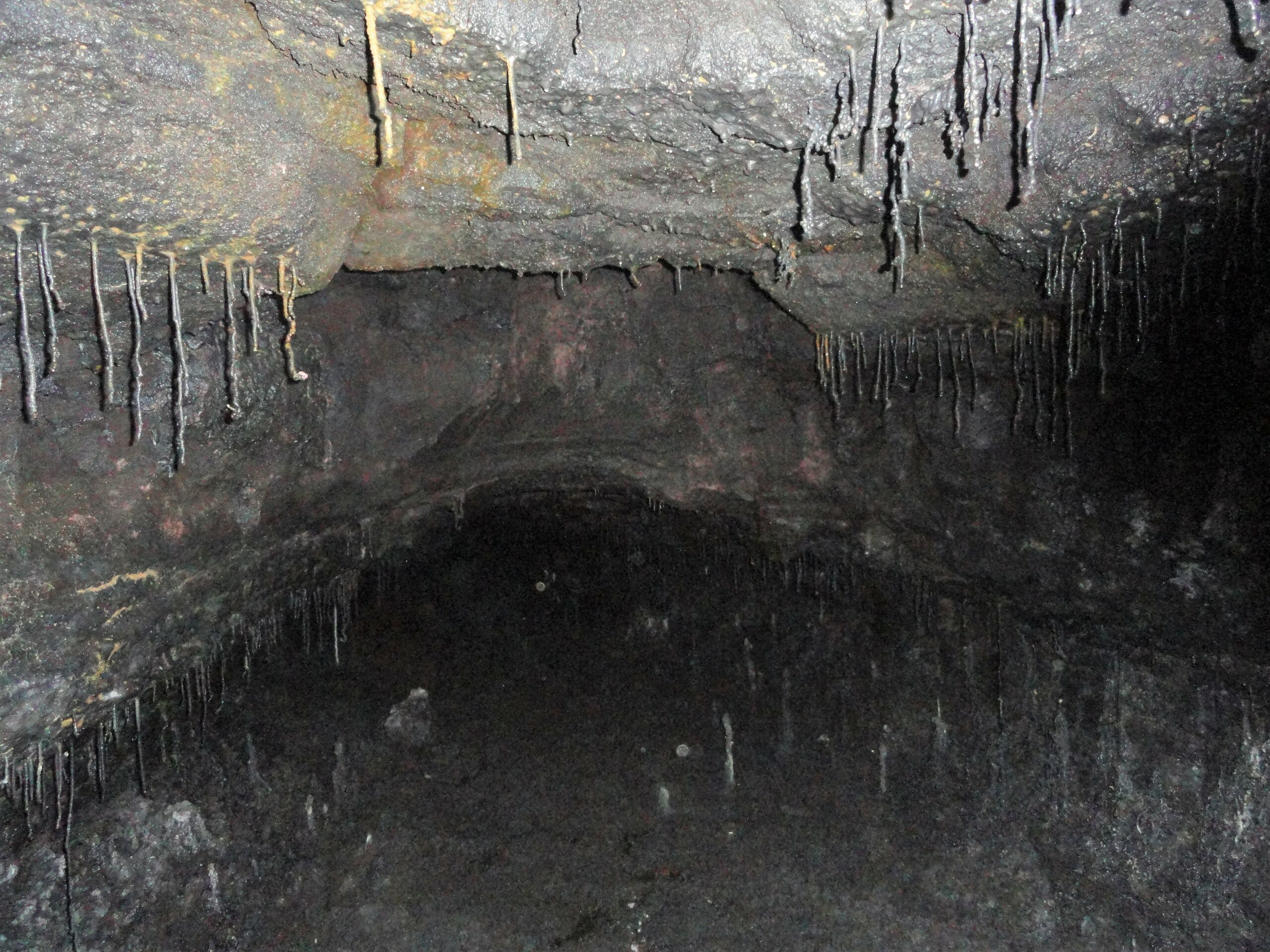
Lava tube caves found in basalt flows (Figure 12.4.1),</li> <li>Ice caves in glaciers,</li> <li>
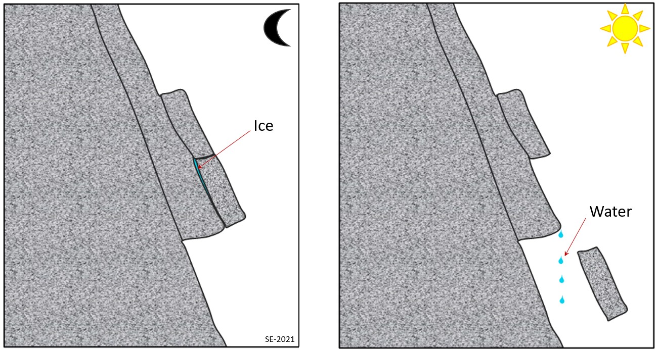
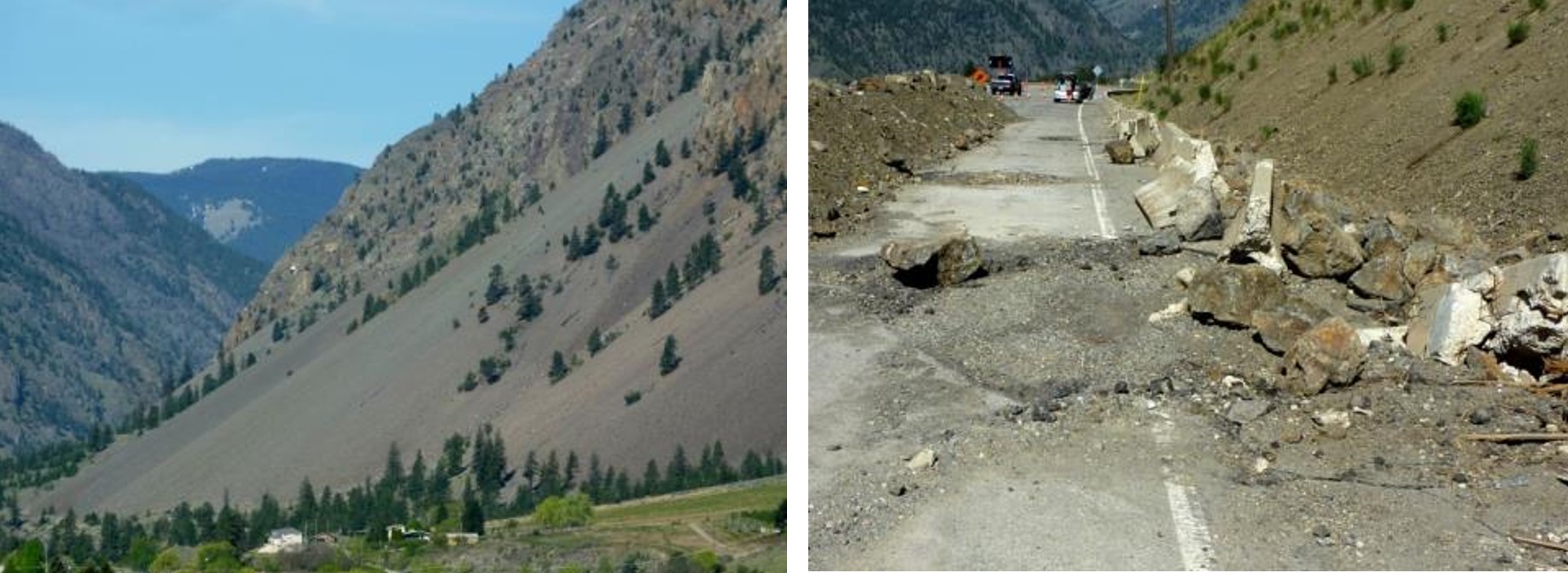
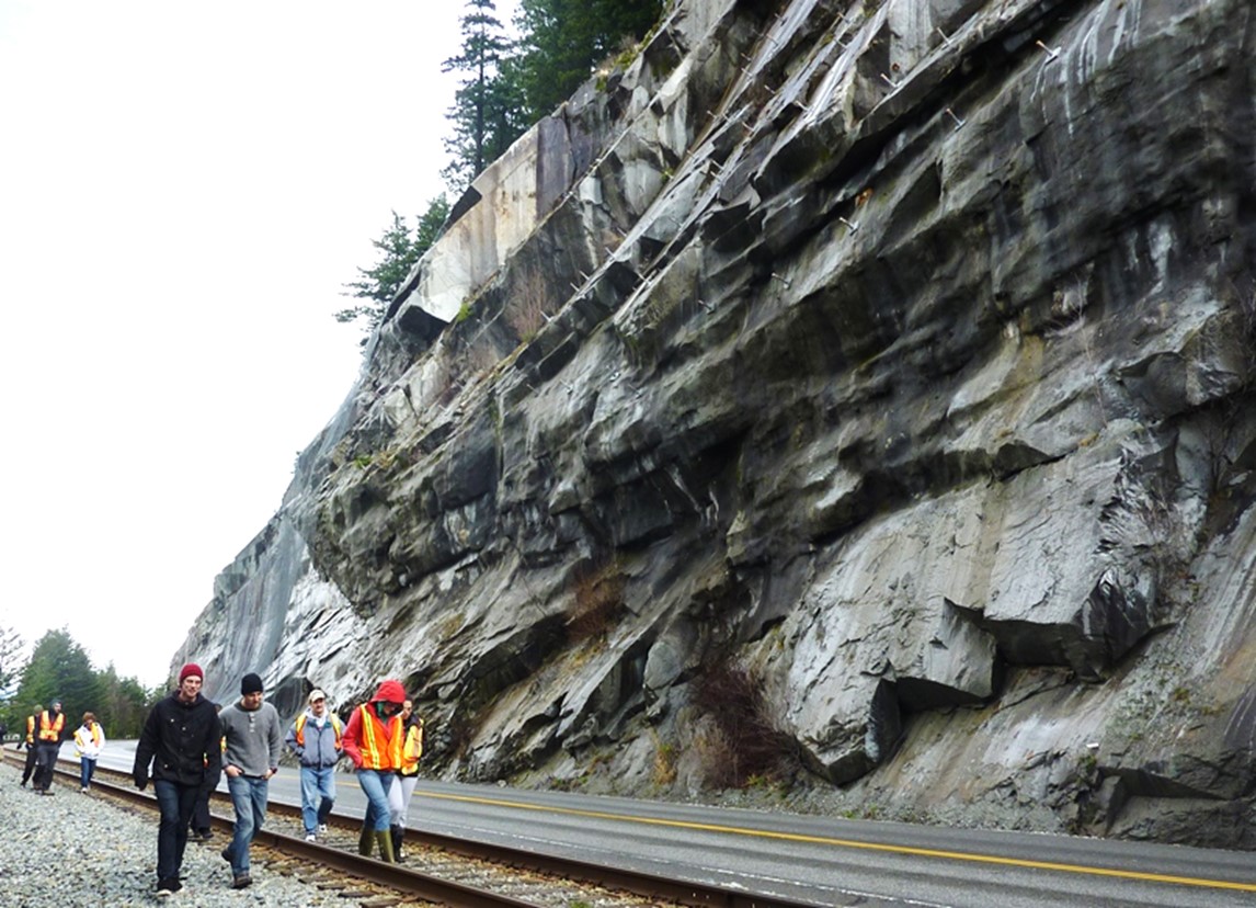
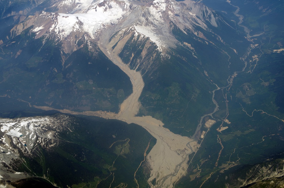
Crevice (or tectonic) caves found along geological faults or folds or formed by mass movement or gravity,</li> <li>Erosional caves formed in softer rocks eroded by water or wind,</li> <li>Littoral or sea caves caused by wave action,</li> <li>
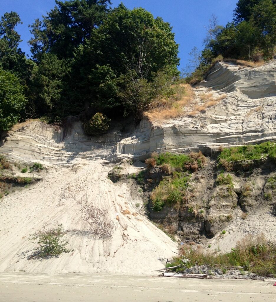
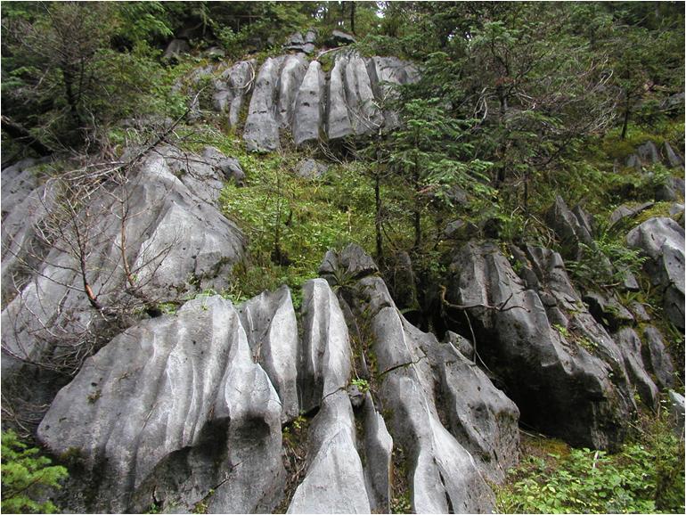
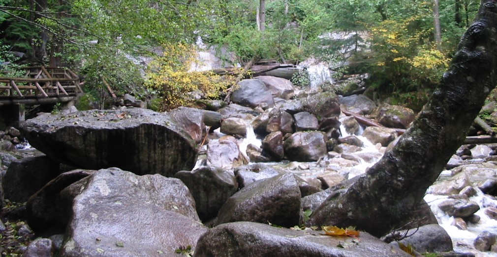
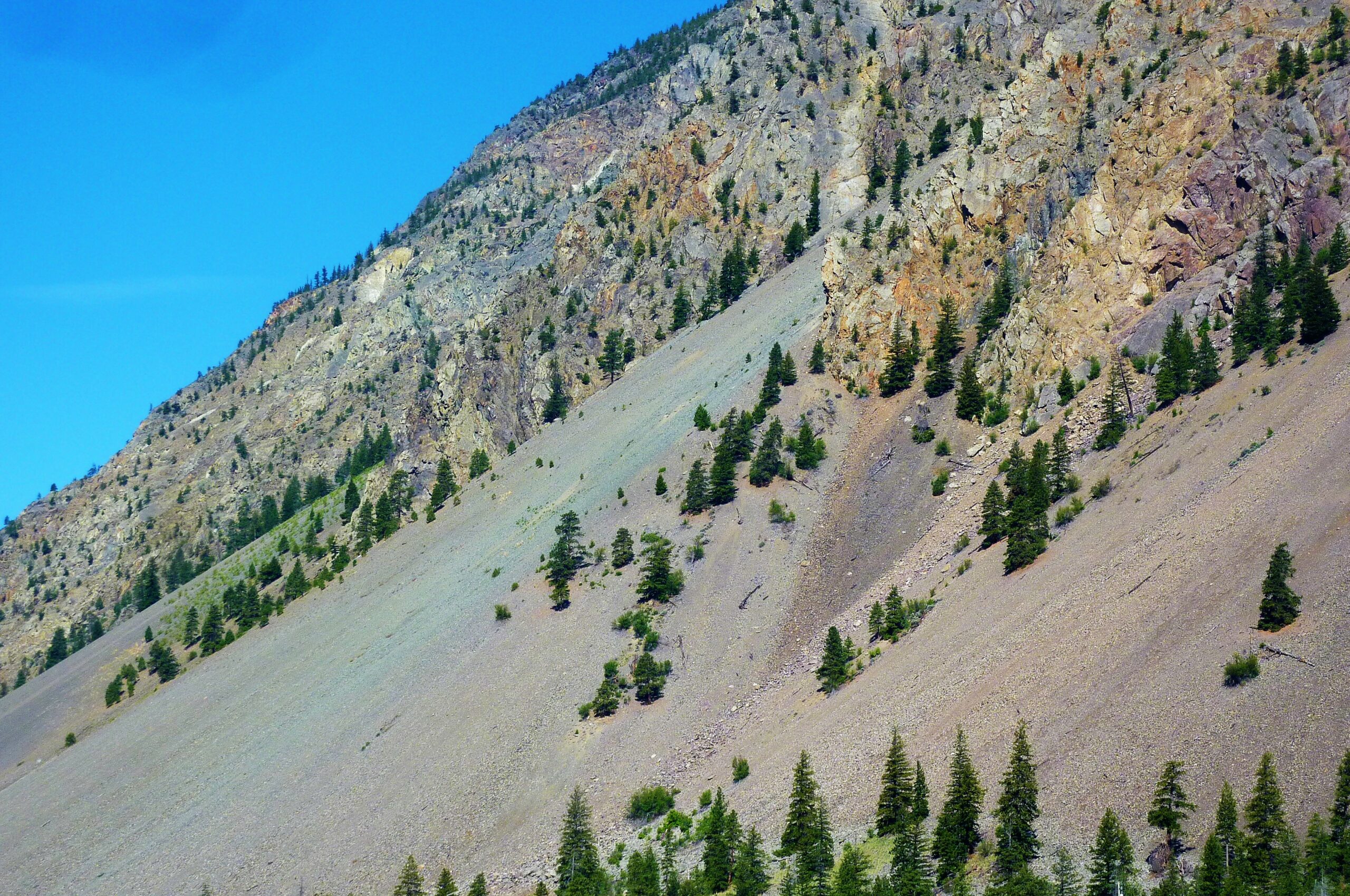
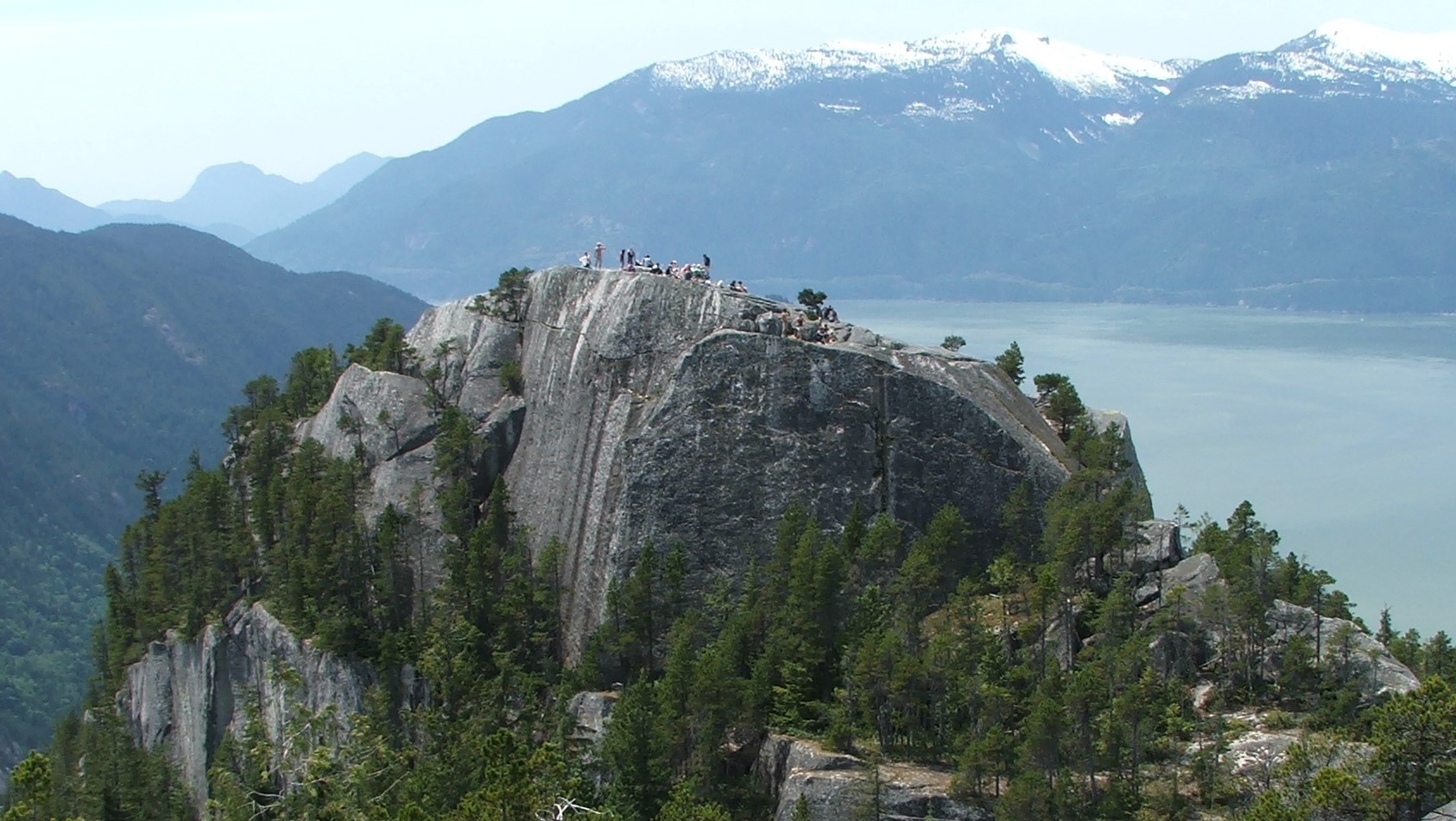
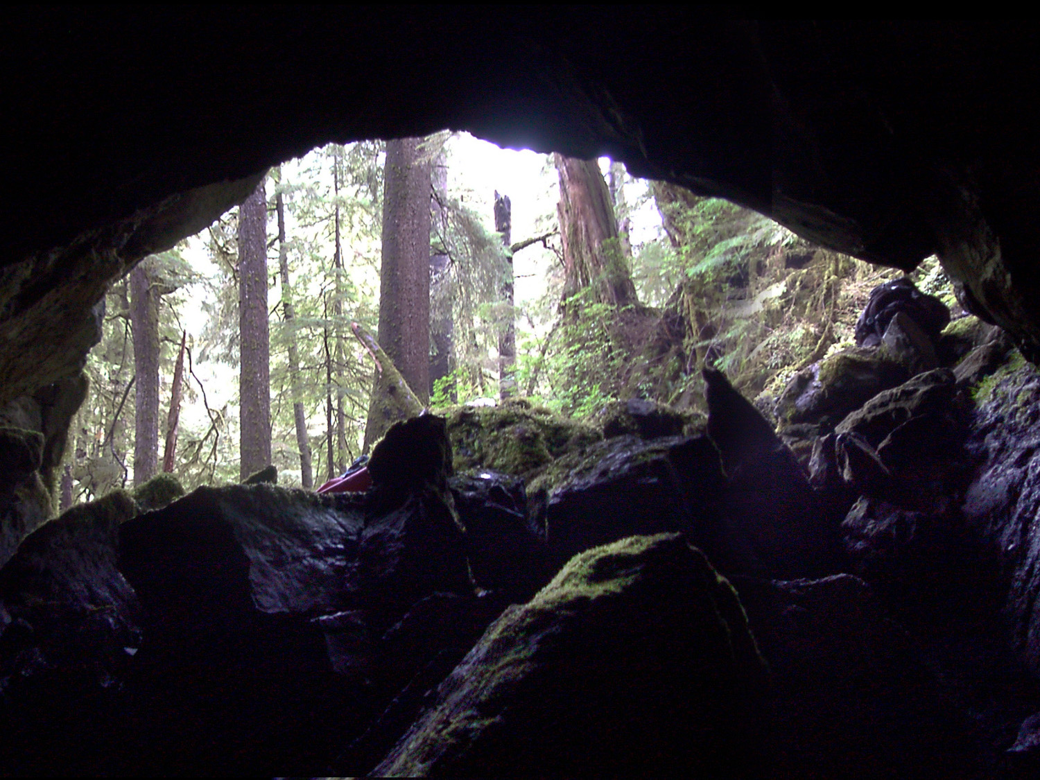
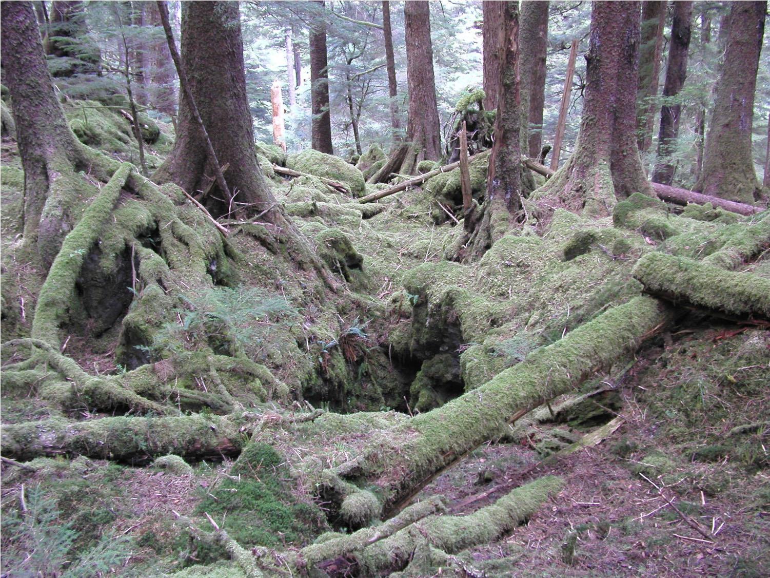
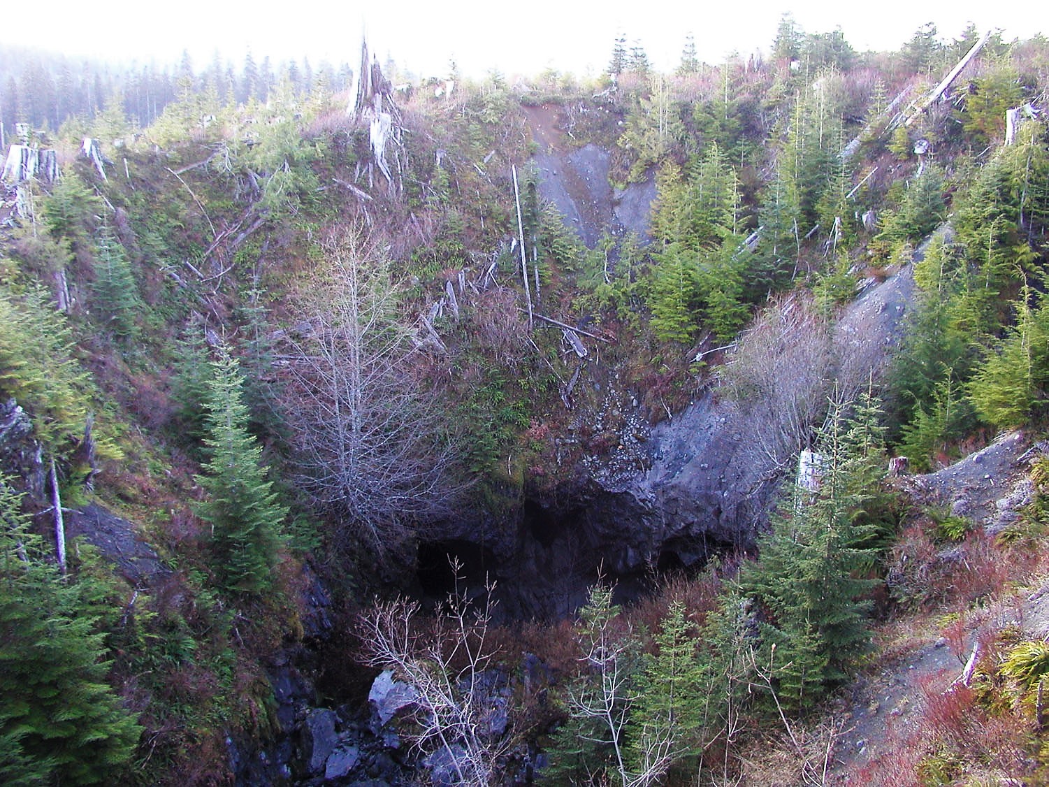
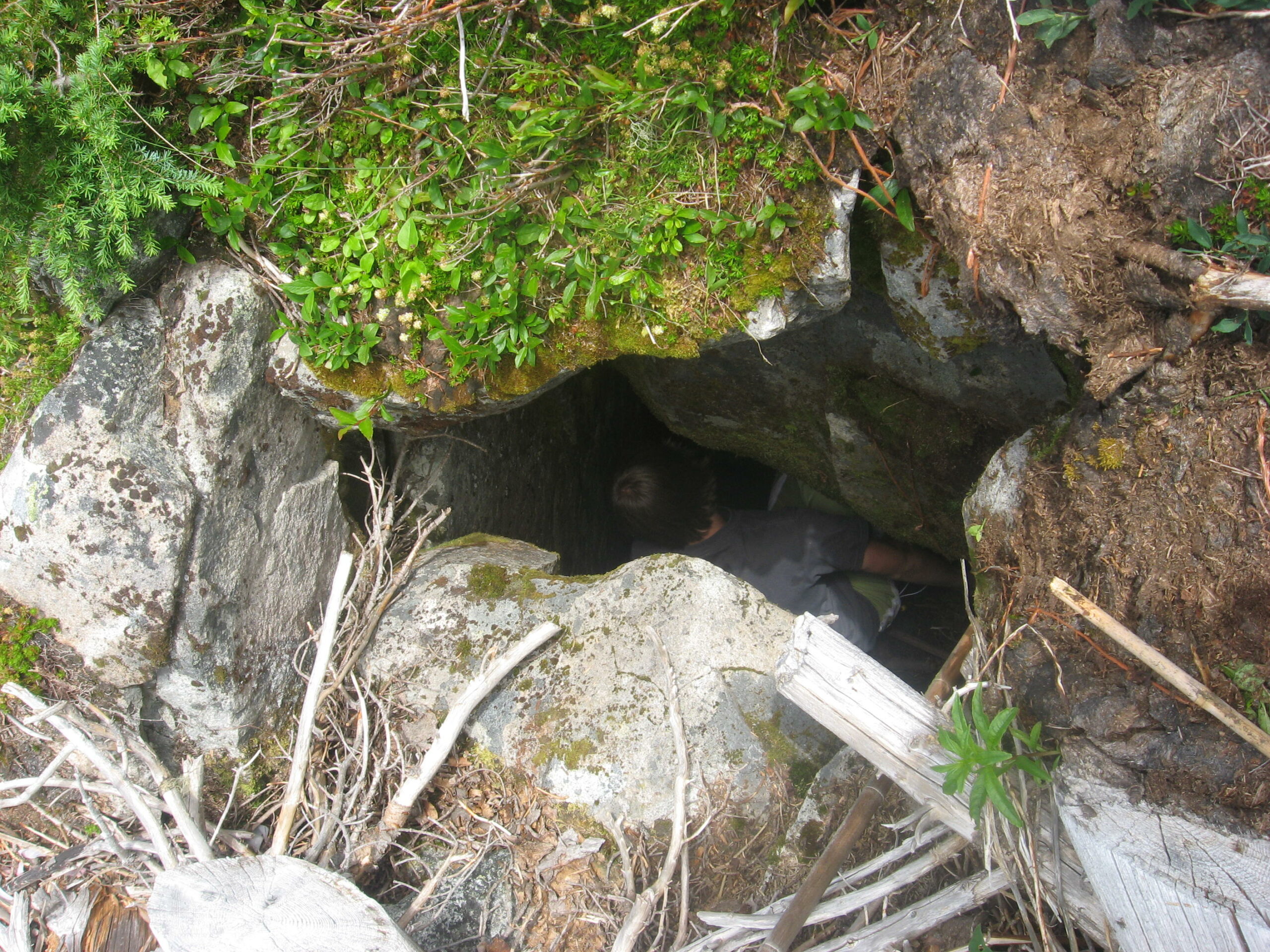
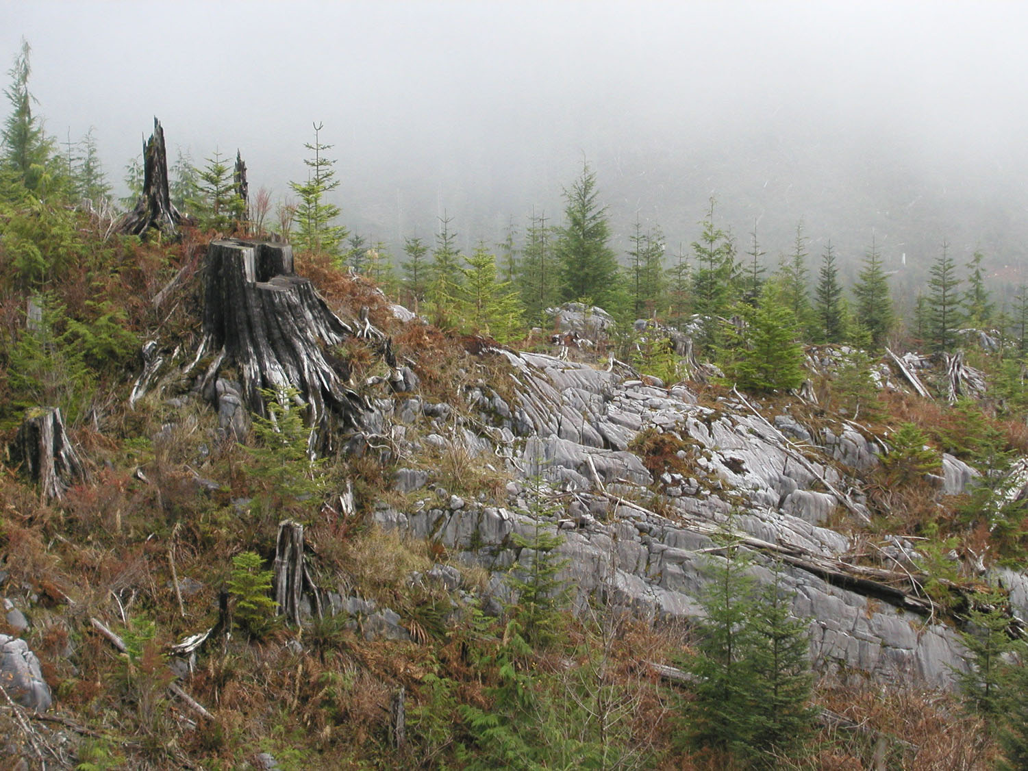
Talus caves under piled rock debris (Figure 12.4.2), and</li> <li>Piping caves formed in unconsolidated materials by the removal of fines by water flow.</li> </ul> <div class="wp-caption aligncenter" id="attachment_826" aria-describedby="caption-attachment-826" style="width: 603px"><a href="http://environmental-geology-dev.pressbooks.tru.ca/wp-content/uploads/sites/73/2021/07/Fig-27-scaled-1.jpg" data-url="http://environmental-geology-dev.pressbooks.tru.ca/wp-content/uploads/sites/73/2021/07/Fig-27-scaled-1.jpg"><img class="wp-image-549" src="http://environmental-geol.pressbooks.tru.ca/wp-content/uploads/sites/123/2021/07/Fig-27-scaled-1.jpg" alt="" width="603" height="453" srcset="https://environmental-geol.pressbooks.tru.ca/wp-content/uploads/sites/123/2021/07/Fig-27-scaled-1.jpg 2560w, https://environmental-geol.pressbooks.tru.ca/wp-content/uploads/sites/123/2021/07/Fig-27-scaled-1-300x225.jpg 300w, https://environmental-geol.pressbooks.tru.ca/wp-content/uploads/sites/123/2021/07/Fig-27-scaled-1-1024x768.jpg 1024w, https://environmental-geol.pressbooks.tru.ca/wp-content/uploads/sites/123/2021/07/Fig-27-scaled-1-768x576.jpg 768w, https://environmental-geol.pressbooks.tru.ca/wp-content/uploads/sites/123/2021/07/Fig-27-scaled-1-1536x1152.jpg 1536w, https://environmental-geol.pressbooks.tru.ca/wp-content/uploads/sites/123/2021/07/Fig-27-scaled-1-2048x1536.jpg 2048w, https://environmental-geol.pressbooks.tru.ca/wp-content/uploads/sites/123/2021/07/Fig-27-scaled-1-65x49.jpg 65w, https://environmental-geol.pressbooks.tru.ca/wp-content/uploads/sites/123/2021/07/Fig-27-scaled-1-225x169.jpg 225w, https://environmental-geol.pressbooks.tru.ca/wp-content/uploads/sites/123/2021/07/Fig-27-scaled-1-350x263.jpg 350w" sizes="(max-width: 603px) 100vw, 603px" title="" /></a><div class="wp-caption-text" id="caption-attachment-826"><strong>Figure 12.4.1</strong> Entering a Lava Tube Cave on the Big Island of Hawaii with Lava Drip Features
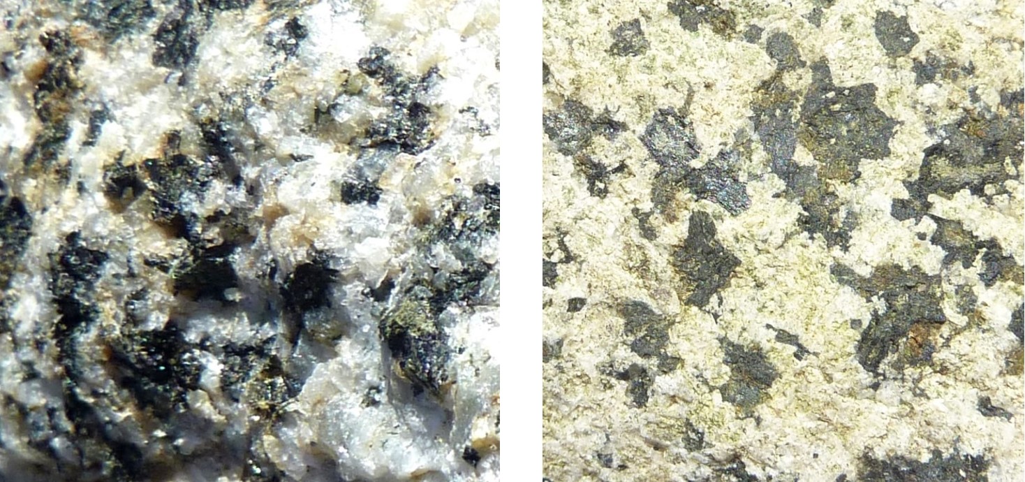
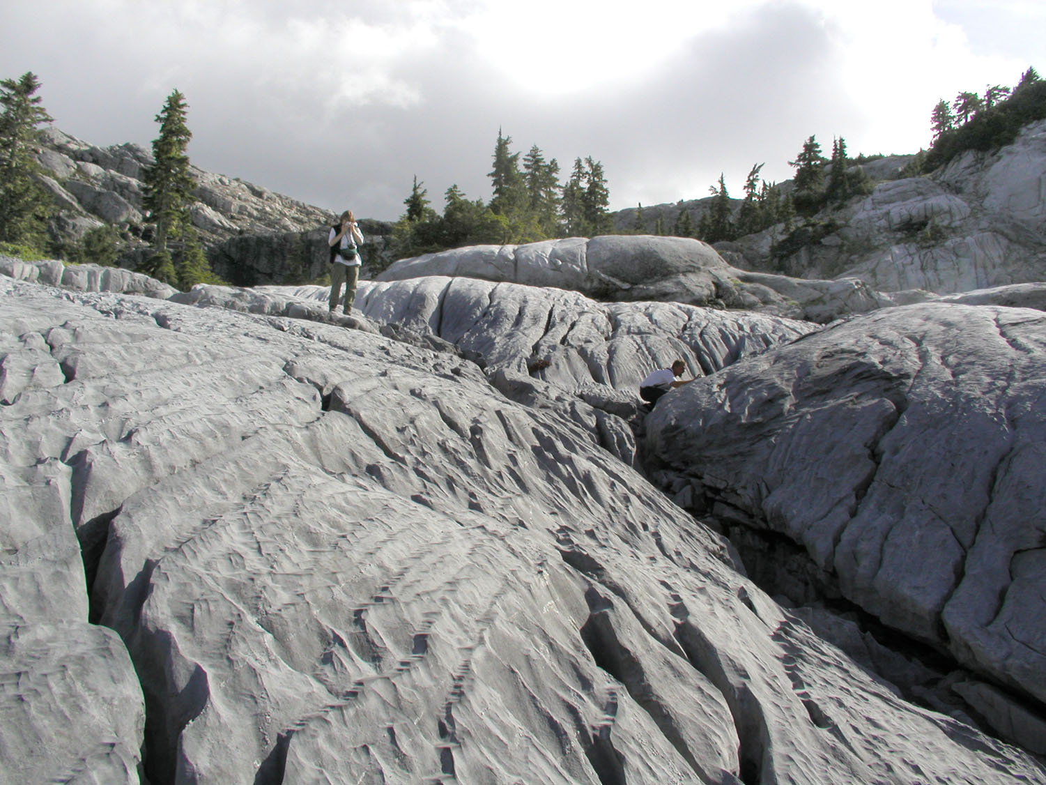
</div></div> <div class="wp-caption aligncenter" id="attachment_866" aria-describedby="caption-attachment-866" style="width: 603px"><a href="http://environmental-geology-dev.pressbooks.tru.ca/wp-content/uploads/sites/73/2021/07/talus-cave-scaled-1.jpg" data-url="http://environmental-geology-dev.pressbooks.tru.ca/wp-content/uploads/sites/73/2021/07/talus-cave-scaled-1.jpg"><img class="wp-image-550" src="http://environmental-geol.pressbooks.tru.ca/wp-content/uploads/sites/123/2022/08/talus-cave-scaled-1.jpg" alt="" width="603" height="453" srcset="https://environmental-geol.pressbooks.tru.ca/wp-content/uploads/sites/123/2022/08/talus-cave-scaled-1.jpg 2560w, https://environmental-geol.pressbooks.tru.ca/wp-content/uploads/sites/123/2022/08/talus-cave-scaled-1-300x225.jpg 300w, https://environmental-geol.pressbooks.tru.ca/wp-content/uploads/sites/123/2022/08/talus-cave-scaled-1-1024x768.jpg 1024w, https://environmental-geol.pressbooks.tru.ca/wp-content/uploads/sites/123/2022/08/talus-cave-scaled-1-768x576.jpg 768w, https://environmental-geol.pressbooks.tru.ca/wp-content/uploads/sites/123/2022/08/talus-cave-scaled-1-1536x1152.jpg 1536w, https://environmental-geol.pressbooks.tru.ca/wp-content/uploads/sites/123/2022/08/talus-cave-scaled-1-2048x1536.jpg 2048w, https://environmental-geol.pressbooks.tru.ca/wp-content/uploads/sites/123/2022/08/talus-cave-scaled-1-65x49.jpg 65w, https://environmental-geol.pressbooks.tru.ca/wp-content/uploads/sites/123/2022/08/talus-cave-scaled-1-225x169.jpg 225w, https://environmental-geol.pressbooks.tru.ca/wp-content/uploads/sites/123/2022/08/talus-cave-scaled-1-350x263.jpg 350w" sizes="(max-width: 603px) 100vw, 603px" title="" /></a><div class="wp-caption-text" id="caption-attachment-866"><strong>Figure 12.4.2</strong> Entrance to a Talus Cave at Mt. Washington, BC.&nbsp; The rock is insoluble granite, not limestone.</div></div> <p>
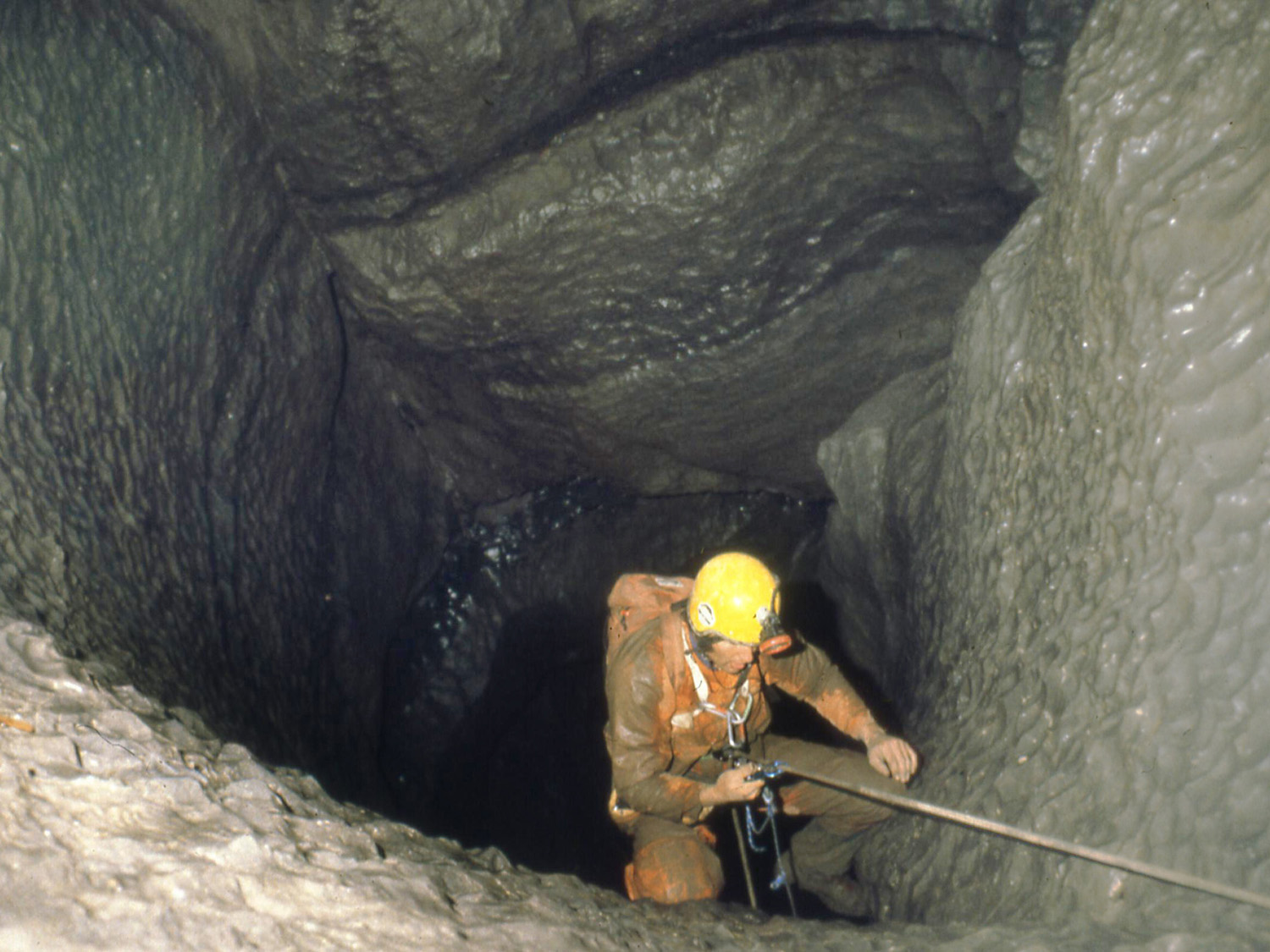
Karst caves may appear as complex or random forms when displayed in maps or cross-sections. However, caves are typically comprised of three fundamental components: passages, chambers, and cave entrances. These components can occur in a whole range of different combinations and permutations. A cave passage can be considered as an elongated element, with a length dimension greater than its height or width. Passages can be horizontal, inclined, or vertical – a vertical passage is usually termed a pitch or pit (Figure 12.4.3). Passages can also be linear (straight), angular, or sinuous:</p> <ul><li>Linear passages typically occur along the strike of the limestone beds,</li> <li>Angular passages can indicate fracture control by joints, and</li> <li>Sinuous passages can be found in flat or gently dipping limestone beds with less fracture control.</li> </ul> <div class="wp-caption aligncenter" id="attachment_452" aria-describedby="caption-attachment-452" style="width: 575px"><a href="http://environmental-geology-dev.pressbooks.tru.ca/wp-content/uploads/sites/73/2021/07/Fig-28.jpg" data-url="http://environmental-geology-dev.pressbooks.tru.ca/wp-content/uploads/sites/73/2021/07/Fig-28.jpg"><img class="wp-image-551" src="http://environmental-geol.pressbooks.tru.ca/wp-content/uploads/sites/123/2022/08/Fig-28-1024x768.jpg" alt="" width="575" height="432" srcset="https://environmental-geol.pressbooks.tru.ca/wp-content/uploads/sites/123/2022/08/Fig-28-1024x768.jpg 1024w, https://environmental-geol.pressbooks.tru.ca/wp-content/uploads/sites/123/2022/08/Fig-28-300x225.jpg 300w, https://environmental-geol.pressbooks.tru.ca/wp-content/uploads/sites/123/2022/08/Fig-28-768x576.jpg 768w, https://environmental-geol.pressbooks.tru.ca/wp-content/uploads/sites/123/2022/08/Fig-28-65x49.jpg 65w, https://environmental-geol.pressbooks.tru.ca/wp-content/uploads/sites/123/2022/08/Fig-28-225x169.jpg 225w, https://environmental-geol.pressbooks.tru.ca/wp-content/uploads/sites/123/2022/08/Fig-28-350x263.jpg 350w, https://environmental-geol.pressbooks.tru.ca/wp-content/uploads/sites/123/2022/08/Fig-28.jpg 1500w" sizes="(max-width: 575px) 100vw, 575px" title="" /></a><div class="wp-caption-text" id="caption-attachment-452"><strong>Figure 12.4.3</strong> Descending Into a Vertical Passage or Pit</div></div> <p>
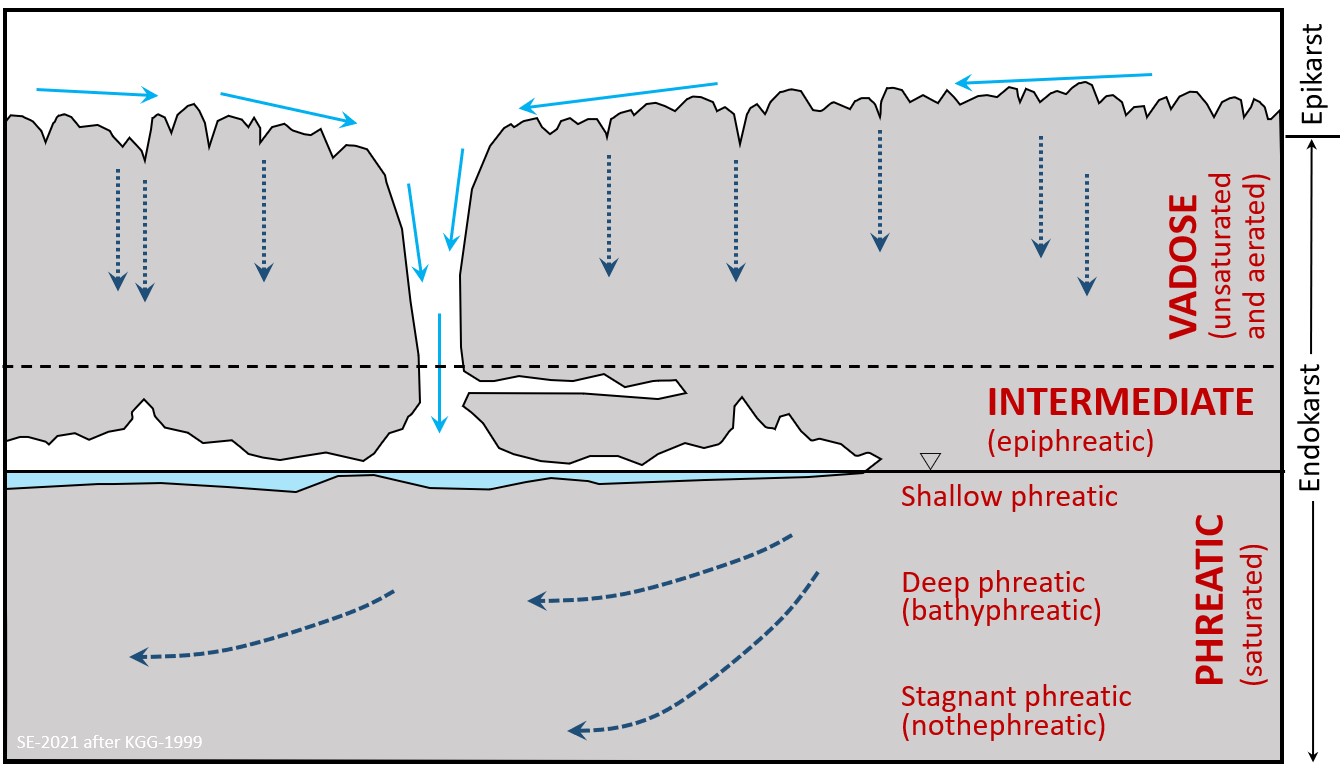
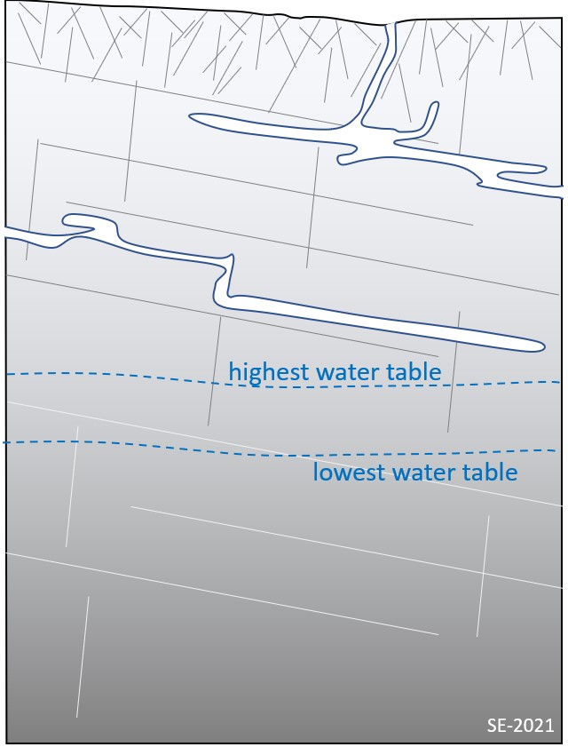
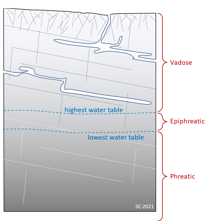
The shape or profile of passages tells us a lot about how the cave formed. Circular, elliptical, or tube-like passages have likely been formed under water-filled (or phreatic) conditions below the water table. More irregular passage profiles are formed above the water table by streams with air space above (vadose conditions). In many cases, passages display evidence of earlier phreatic (aerated) phases overprinted by subsequent vadose (flooded) ones. A great example of this is a keyhole passage – where a phreatic tube has been incised by a vadose channel. Other major constraints on passage shape are:</p> <ul><li>The orientation of bedding planes and joints,</li> <li>The infilling of the passage with introduced sediments, and</li> <li>Cave breakdown material.</li> </ul> <p>
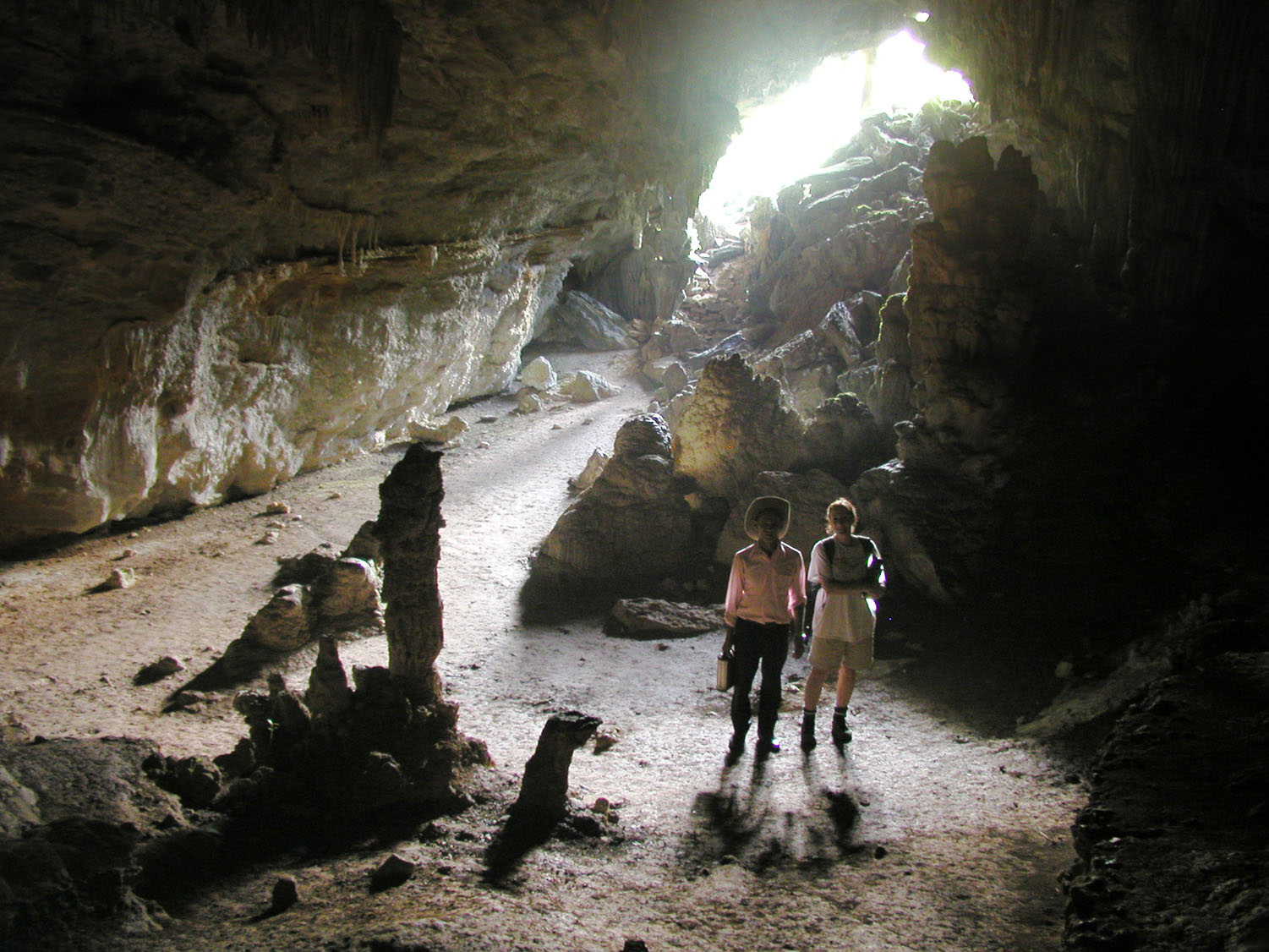
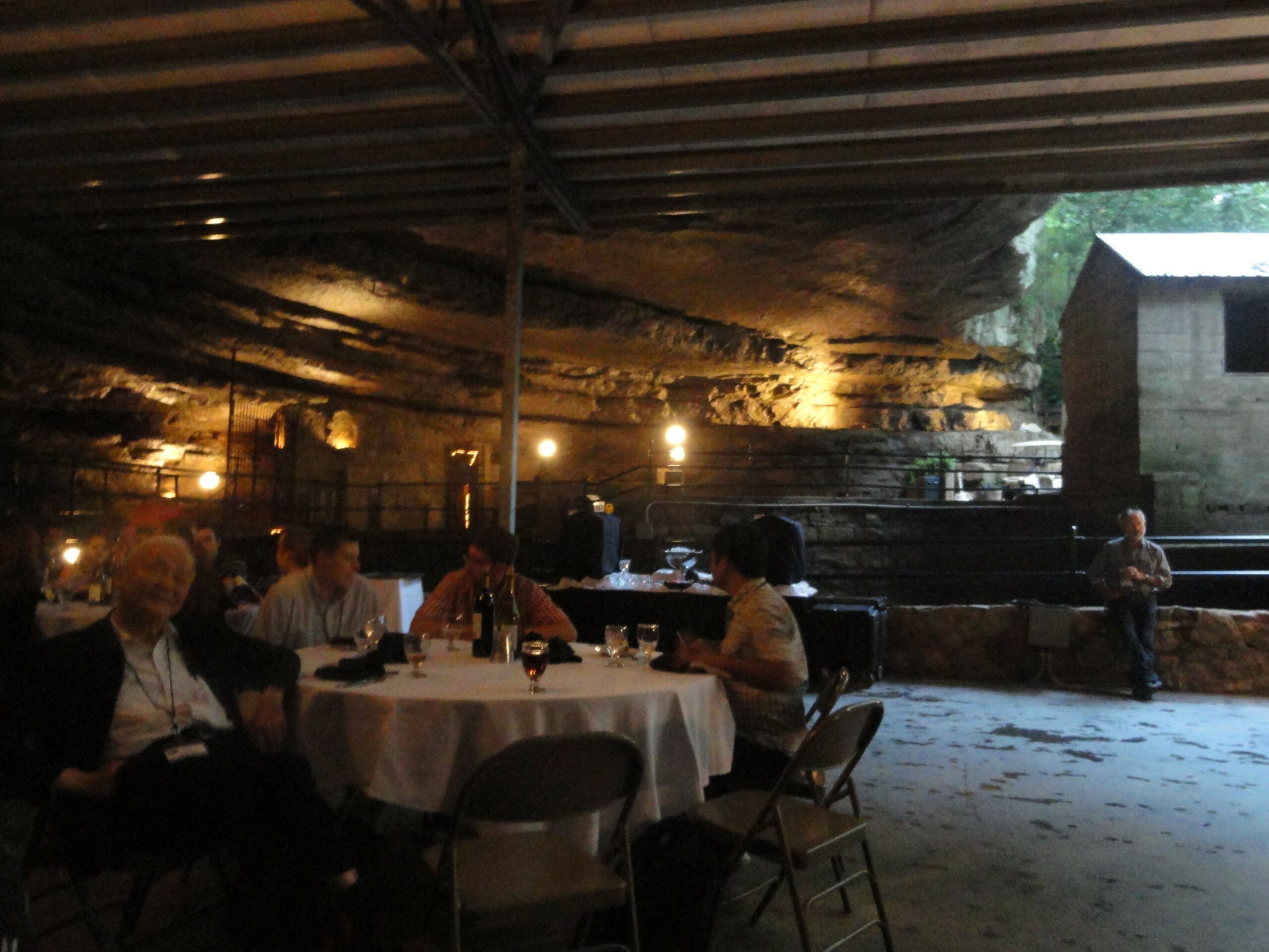
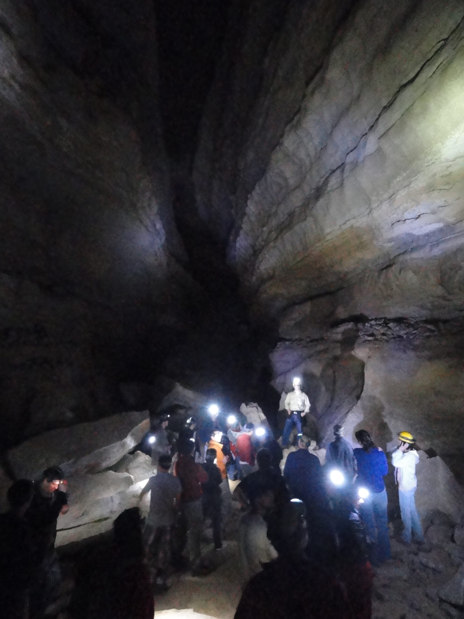
Chambers, or rooms, are localized sites of cave passage enlargement where there is a significant increase in height or width of the passage. Chambers may form due to the intersection of two or more passages or where preferential erosion has occurred; e.g., extensive breakdown of the ceiling (Figure 12.4.4). One of the largest chambers known is at Mulu Caves in Sarawak (Borneo), where there is a 700 m long, 400 m wide and &gt; 70 m high chamber. Chambers can also form by the upwelling of hydrothermal solutions.
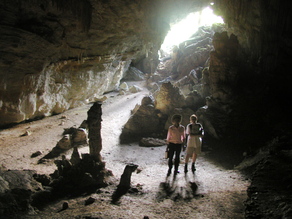
</p> <div class="wp-caption aligncenter" id="attachment_453" aria-describedby="caption-attachment-453" style="width: 663px"><a href="http://environmental-geology-dev.pressbooks.tru.ca/wp-content/uploads/sites/73/2021/07/Fig-29.jpg" data-url="http://environmental-geology-dev.pressbooks.tru.ca/wp-content/uploads/sites/73/2021/07/Fig-29.jpg"><img class="wp-image-552" src="http://environmental-geol.pressbooks.tru.ca/wp-content/uploads/sites/123/2022/08/Fig-29-1024x768.jpg" alt="" width="663" height="498" srcset="https://environmental-geol.pressbooks.tru.ca/wp-content/uploads/sites/123/2022/08/Fig-29-1024x768.jpg 1024w, https://environmental-geol.pressbooks.tru.ca/wp-content/uploads/sites/123/2022/08/Fig-29-300x225.jpg 300w, https://environmental-geol.pressbooks.tru.ca/wp-content/uploads/sites/123/2022/08/Fig-29-768x576.jpg 768w, https://environmental-geol.pressbooks.tru.ca/wp-content/uploads/sites/123/2022/08/Fig-29-65x49.jpg 65w, https://environmental-geol.pressbooks.tru.ca/wp-content/uploads/sites/123/2022/08/Fig-29-225x169.jpg 225w, https://environmental-geol.pressbooks.tru.ca/wp-content/uploads/sites/123/2022/08/Fig-29-350x263.jpg 350w, https://environmental-geol.pressbooks.tru.ca/wp-content/uploads/sites/123/2022/08/Fig-29.jpg 1501w" sizes="(max-width: 663px) 100vw, 663px" title="" /></a><div class="wp-caption-text" id="caption-attachment-453"><strong>Figure 12.4.4</strong> Large Chamber Near Entrance to Tropical Cave in Cuba</div></div> <p>All caves that are entered by humans have openings or entrances unless a man-made opening has been made into a cave. Cave entrances do not necessarily play a significant role in cave development unless they capture a sinking or discharge a rising stream. Caves can quite easily develop without enterable entrances, and entrances may form later in the life of a cave as the overlying landscape is eroded and openings (or windows) into underlying caves occur. Individual caves in any given area may be hydrologically linked to other nearby caves forming a network of passages, chambers, and conduits. These caves then become part of what is known as a cave system.</p> <h1>Cave Speleogens and Speleothems</h1> <p>Speleogens are the rocky relief features in caves while speleothems are the mineral formations present in caves. Mineral formations differ from cave sediments in that they only form inside the caves, while cave sediments from materials inside caves (autochonous) and also from materials bought from the outside to the inside of caves (allochthonous).<br /> Speleogens as rocky relief features are centimetre to metre-scale and are found on the interior surfaces of caves and are the result of chemical dissolution, mechanical erosion, or a combination of both; and are useful in interpreting the cave’s history and genesis. Speleogens can include:</p> <ul><li>Linear grooves or flutes on steep surfaces,</li> <li>Canyons and incised meanders,</li> <li>Recessions and depressions on the passage floor, ceiling, or sidewall walls of caves forming scallops, potholes and spongework,</li> <li>
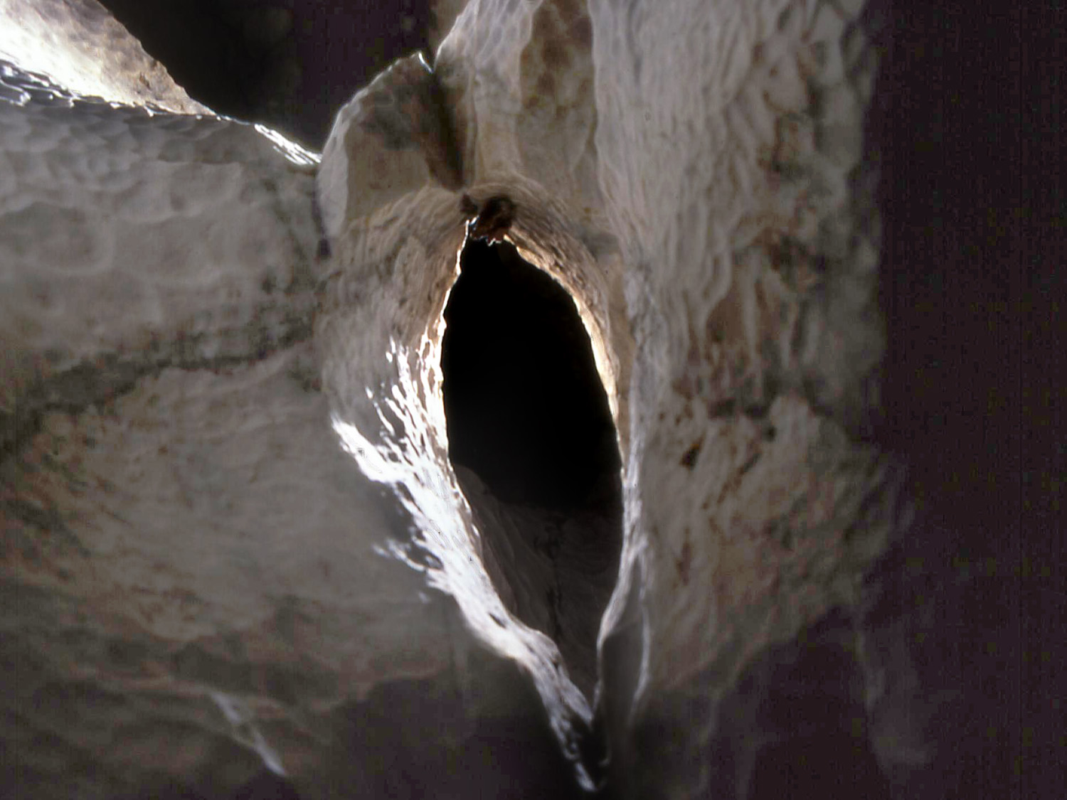
Horizontal slots on side walls including notches or bevels (Figure 12.4.5), and</li> <li>Protuberances in cave passages, such as pendants, knife edges, spikes, and pillars.</li> </ul> <div class="wp-caption aligncenter" id="attachment_454" aria-describedby="caption-attachment-454" style="width: 610px"><a href="http://environmental-geology-dev.pressbooks.tru.ca/wp-content/uploads/sites/73/2021/07/Fig-30.jpg" data-url="http://environmental-geology-dev.pressbooks.tru.ca/wp-content/uploads/sites/73/2021/07/Fig-30.jpg"><img class="wp-image-553" src="http://environmental-geol.pressbooks.tru.ca/wp-content/uploads/sites/123/2022/08/Fig-30-1024x768.jpg" alt="" width="610" height="458" srcset="https://environmental-geol.pressbooks.tru.ca/wp-content/uploads/sites/123/2022/08/Fig-30-1024x768.jpg 1024w, https://environmental-geol.pressbooks.tru.ca/wp-content/uploads/sites/123/2022/08/Fig-30-300x225.jpg 300w, https://environmental-geol.pressbooks.tru.ca/wp-content/uploads/sites/123/2022/08/Fig-30-768x576.jpg 768w, https://environmental-geol.pressbooks.tru.ca/wp-content/uploads/sites/123/2022/08/Fig-30-65x49.jpg 65w, https://environmental-geol.pressbooks.tru.ca/wp-content/uploads/sites/123/2022/08/Fig-30-225x169.jpg 225w, https://environmental-geol.pressbooks.tru.ca/wp-content/uploads/sites/123/2022/08/Fig-30-350x263.jpg 350w, https://environmental-geol.pressbooks.tru.ca/wp-content/uploads/sites/123/2022/08/Fig-30.jpg 1500w" sizes="(max-width: 610px) 100vw, 610px" title="" /></a><div class="wp-caption-text" id="caption-attachment-454"><strong>Figure 12.4.5</strong> Part of an Erosional Slot Developing on the Side of a Cave Protuberance, Such as a Pillar.</div></div> <p>
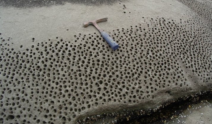
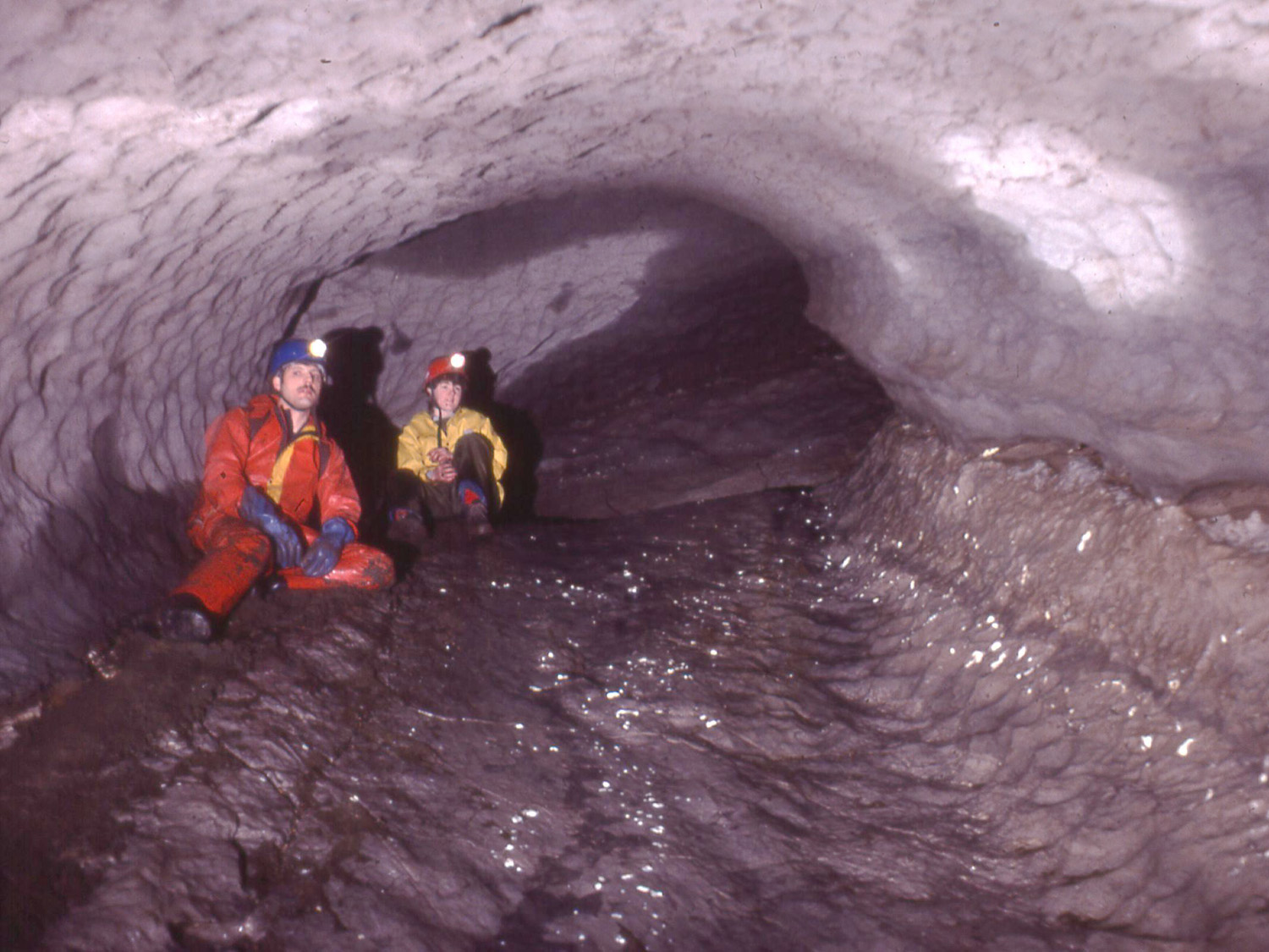
Scallops are spoon-shaped hollows are formed by eddies in water flow and vary from a centimetre to a metre in size and have a distinct asymmetry (Figure 12.4.6). The steeper side indicates the upstream direction of paleoflow. The size of the scallops can also tell us something about the speed of the flow – the smaller the scallop the greater the flow. Potholes are circular basins centimetres to a metre in diameter that occur along stream beds in cave passages. Potholes develop where there is rapid water flow combined with rock fragments that grind into the bedrock in a swirling motion. Spongework are where random holes or cavities are present on the walls or ceiling of the cave and develop under phreatic conditions in slow moving and swirling water flow.</p> <div class="wp-caption aligncenter" id="attachment_455" aria-describedby="caption-attachment-455" style="width: 623px"><a href="http://environmental-geology-dev.pressbooks.tru.ca/wp-content/uploads/sites/73/2021/07/Fig-31.jpg" data-url="http://environmental-geology-dev.pressbooks.tru.ca/wp-content/uploads/sites/73/2021/07/Fig-31.jpg"><img class="wp-image-554" src="http://environmental-geol.pressbooks.tru.ca/wp-content/uploads/sites/123/2022/08/Fig-31-1024x768.jpg" alt="" width="623" height="468" srcset="https://environmental-geol.pressbooks.tru.ca/wp-content/uploads/sites/123/2022/08/Fig-31-1024x768.jpg 1024w, https://environmental-geol.pressbooks.tru.ca/wp-content/uploads/sites/123/2022/08/Fig-31-300x225.jpg 300w, https://environmental-geol.pressbooks.tru.ca/wp-content/uploads/sites/123/2022/08/Fig-31-768x576.jpg 768w, https://environmental-geol.pressbooks.tru.ca/wp-content/uploads/sites/123/2022/08/Fig-31-65x49.jpg 65w, https://environmental-geol.pressbooks.tru.ca/wp-content/uploads/sites/123/2022/08/Fig-31-225x169.jpg 225w, https://environmental-geol.pressbooks.tru.ca/wp-content/uploads/sites/123/2022/08/Fig-31-350x263.jpg 350w, https://environmental-geol.pressbooks.tru.ca/wp-content/uploads/sites/123/2022/08/Fig-31.jpg 1500w" sizes="(max-width: 623px) 100vw, 623px" title="" /></a><div class="wp-caption-text" id="caption-attachment-455"><strong>Figure 12.4.6</strong> Scallops Along the Sides of an Inclined Cave Passage, Which is Also a Phreatic Tube</div></div> <p>
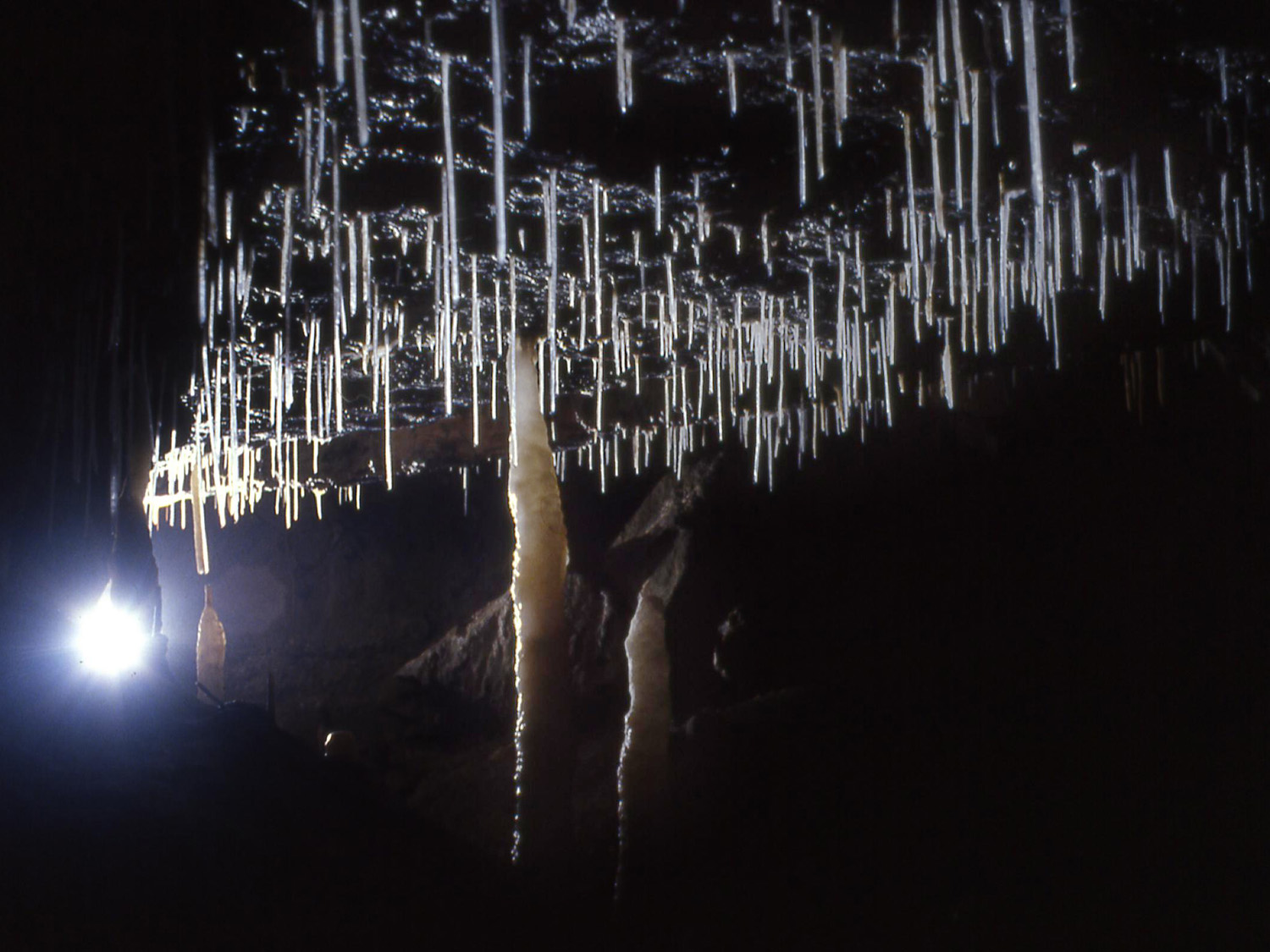
Speleothems are cave mineral formations or decorations (Figure 12.4.7). Stalactites (which are attached to ceilings and ledges and grow downward) and stalagmites (which grow upward from the cave floor) are probably the best-known examples of cave decorations. Many other kinds of speleothems have been identified and vary widely in size, form, and chemical composition. Despite this, they all have one thing in common – they are all secondary compounds that have either: been formed because of some chemical interaction with cave substrates or have been precipitated out of karst system waters under subterranean conditions. Given limestone’s chemical composition, the most prevalent cave minerals are forms of calcium carbonate. The arrangement of atoms within calcium carbonate can combine in three ways, producing three minerals: calcite, aragonite, or vaterite. These minerals (also called polymorphs) are identical in terms of their chemical composition, but differ in terms of their crystalline structure, and stability. Most calcite formations are colourless or white, but the presence of certain impurities, or chromophores, can have impart on the various colours or degrees of opacity to speleothems (e.g., brownish yellow associated with iron oxide).
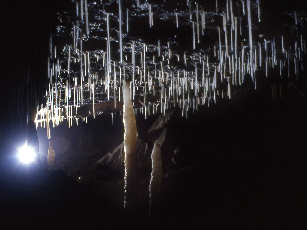
</p> <div class="wp-caption aligncenter" id="attachment_456" aria-describedby="caption-attachment-456" style="width: 653px"><a href="http://environmental-geology-dev.pressbooks.tru.ca/wp-content/uploads/sites/73/2021/07/Fig-32.jpg" data-url="http://environmental-geology-dev.pressbooks.tru.ca/wp-content/uploads/sites/73/2021/07/Fig-32.jpg"><img class="wp-image-555" src="http://environmental-geol.pressbooks.tru.ca/wp-content/uploads/sites/123/2022/08/Fig-32-1024x768.jpg" alt="" width="653" height="490" srcset="https://environmental-geol.pressbooks.tru.ca/wp-content/uploads/sites/123/2022/08/Fig-32-1024x768.jpg 1024w, https://environmental-geol.pressbooks.tru.ca/wp-content/uploads/sites/123/2022/08/Fig-32-300x225.jpg 300w, https://environmental-geol.pressbooks.tru.ca/wp-content/uploads/sites/123/2022/08/Fig-32-768x576.jpg 768w, https://environmental-geol.pressbooks.tru.ca/wp-content/uploads/sites/123/2022/08/Fig-32-65x49.jpg 65w, https://environmental-geol.pressbooks.tru.ca/wp-content/uploads/sites/123/2022/08/Fig-32-225x169.jpg 225w, https://environmental-geol.pressbooks.tru.ca/wp-content/uploads/sites/123/2022/08/Fig-32-350x263.jpg 350w, https://environmental-geol.pressbooks.tru.ca/wp-content/uploads/sites/123/2022/08/Fig-32.jpg 1500w" sizes="(max-width: 653px) 100vw, 653px" title="" /></a><div class="wp-caption-text" id="caption-attachment-456"><strong>Figure 12.4.7</strong> Soda Straws, Stalagmites, and Column, Along With Cave Sediment on Floor of Cave Passage</div></div> <p>Speleothems form when the calcium carbonate-saturated water emerges into underground opening or caves and meets air. Under these conditions carbon dioxide is released from the water into the cave atmosphere, reducing the carbonic acid level of the water, and calcium carbonate will begin to precipitate out of the water. Calcium carbonate is only readily soluble in pure water if the water is acidic. As the carbon dioxide level of the water decreases, the acidity will also decrease along with the solubility of calcium carbonate. In drier caves evaporation might also play a role leaving behind deposits of calcium carbonate in the form of calcite or aragonite. There are also other ways for the carbon dioxide content of water to be diminished and for calcite to be deposit, such as by increasing the temperature of the water (lessening the solubility of the carbon dioxide) and by the actions of certain bacteria.</p> <p>
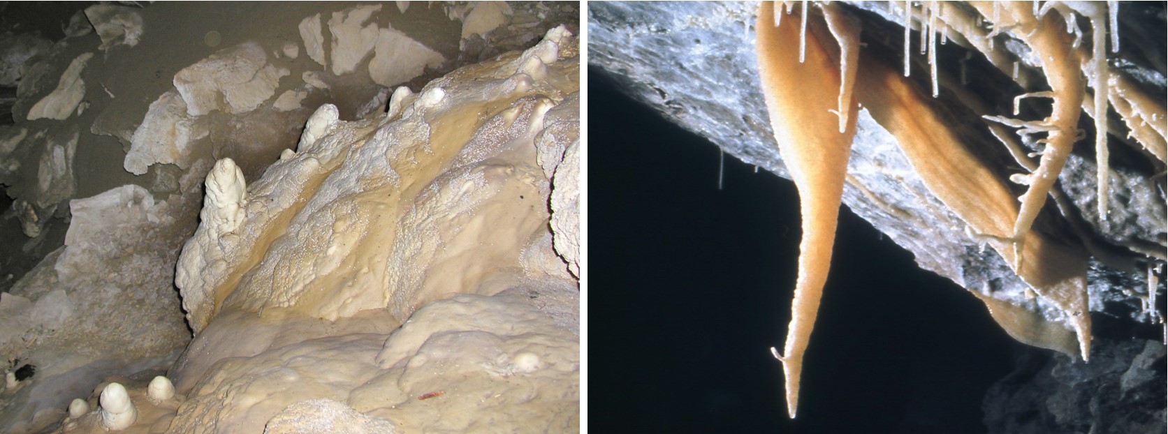
Cave mineral formations can be grouped under three broad categories: dripstone and flowstone forms, erratic forms, and sub-aqueous forms. Dripstone and flowstones include the types of formations most people are familiar with and typically associate with caves including stalactites, stalagmites, flowstone, draperies, and columns (Figure 12.4.8). These formations can take an astonishing variety of sizes, shapes, and forms. The other two categories represent formations that may be less familiar. Erratic forms include shields, helectites, botryoidal forms, anthodites and moonmilk. While sub-aqueous forms include rimstone pools, concretions, pool deposits and crystal linings (Figure 12.4.9).
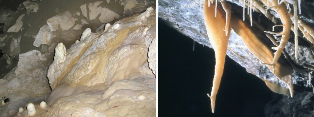
</p> <div class="wp-caption aligncenter" id="attachment_457" aria-describedby="caption-attachment-457" style="width: 733px"><a href="http://environmental-geology-dev.pressbooks.tru.ca/wp-content/uploads/sites/73/2021/07/flowstone-helictite.jpg" data-url="http://environmental-geology-dev.pressbooks.tru.ca/wp-content/uploads/sites/73/2021/07/flowstone-helictite.jpg"><img class="wp-image-556" src="http://environmental-geol.pressbooks.tru.ca/wp-content/uploads/sites/123/2022/08/flowstone-helictite-1024x381.jpg" alt="" width="733" height="273" srcset="https://environmental-geol.pressbooks.tru.ca/wp-content/uploads/sites/123/2022/08/flowstone-helictite-1024x381.jpg 1024w, https://environmental-geol.pressbooks.tru.ca/wp-content/uploads/sites/123/2022/08/flowstone-helictite-300x112.jpg 300w, https://environmental-geol.pressbooks.tru.ca/wp-content/uploads/sites/123/2022/08/flowstone-helictite-768x286.jpg 768w, https://environmental-geol.pressbooks.tru.ca/wp-content/uploads/sites/123/2022/08/flowstone-helictite-1536x571.jpg 1536w, https://environmental-geol.pressbooks.tru.ca/wp-content/uploads/sites/123/2022/08/flowstone-helictite-65x24.jpg 65w, https://environmental-geol.pressbooks.tru.ca/wp-content/uploads/sites/123/2022/08/flowstone-helictite-225x84.jpg 225w, https://environmental-geol.pressbooks.tru.ca/wp-content/uploads/sites/123/2022/08/flowstone-helictite-350x130.jpg 350w, https://environmental-geol.pressbooks.tru.ca/wp-content/uploads/sites/123/2022/08/flowstone-helictite.jpg 1672w" sizes="(max-width: 733px) 100vw, 733px" title="" /></a><div class="wp-caption-text" id="caption-attachment-457"><strong>Figure 12.4.8</strong> Flowstone Forming Along Fracture (left), and Soda Straws and Helictite-Type Features Forming on the Roof of Cave Passage (right)
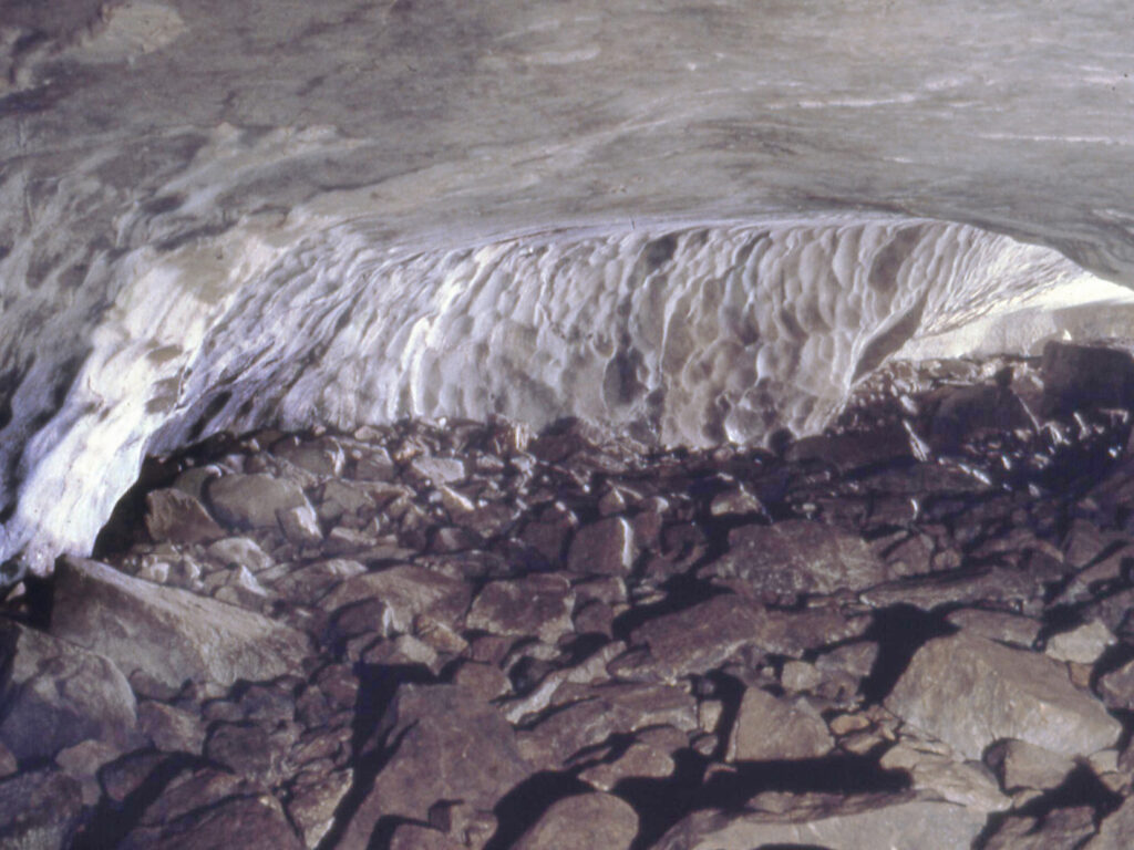
</div></div> <div class="wp-caption aligncenter" id="attachment_458" aria-describedby="caption-attachment-458" style="width: 525px"><a href="http://environmental-geology-dev.pressbooks.tru.ca/wp-content/uploads/sites/73/2021/07/Fig-35.jpg" data-url="http://environmental-geology-dev.pressbooks.tru.ca/wp-content/uploads/sites/73/2021/07/Fig-35.jpg"><img class="wp-image-557" src="http://environmental-geol.pressbooks.tru.ca/wp-content/uploads/sites/123/2022/08/Fig-35-1024x768.jpg" alt="" width="525" height="394" srcset="https://environmental-geol.pressbooks.tru.ca/wp-content/uploads/sites/123/2022/08/Fig-35-1024x768.jpg 1024w, https://environmental-geol.pressbooks.tru.ca/wp-content/uploads/sites/123/2022/08/Fig-35-300x225.jpg 300w, https://environmental-geol.pressbooks.tru.ca/wp-content/uploads/sites/123/2022/08/Fig-35-768x576.jpg 768w, https://environmental-geol.pressbooks.tru.ca/wp-content/uploads/sites/123/2022/08/Fig-35-65x49.jpg 65w, https://environmental-geol.pressbooks.tru.ca/wp-content/uploads/sites/123/2022/08/Fig-35-225x169.jpg 225w, https://environmental-geol.pressbooks.tru.ca/wp-content/uploads/sites/123/2022/08/Fig-35-350x263.jpg 350w, https://environmental-geol.pressbooks.tru.ca/wp-content/uploads/sites/123/2022/08/Fig-35.jpg 1500w" sizes="(max-width: 525px) 100vw, 525px" title="" /></a><div class="wp-caption-text" id="caption-attachment-458"><strong>Figure 12.4.9</strong> Rim Stone Pool Formation from the Skocjan Caves, Slovenia</div></div> <p>It is very important to understand that speleothems are not just static and ‘pretty’ formations; they are dynamic structures, resulting from natural processes operating in the underground environment and in the broader karst system. If these processes are interrupted or altered, speleothems may be affected, sometimes with unfortunate consequences. Remember too that the calcite deposition process is reversible, and that these formations can be re-dissolved if they are exposed to water that is slightly acidic.</p> <p>The rate of speleothem growth is quite variable and is based on many factors, including: climatic conditions on the surface and underground, groundwater flow rates and characteristics, drip-water composition, microbial activity, size and nature of underground openings, and carbon dioxide concentrations. If the amount of water percolating down through the soil is reduced, due to arid or extremely cold conditions on the surface, calcite deposition may slow down or stop altogether. Calcite deposition rates tend to be greatest in environments that are continually warm and wet. Different types of speleothems grow at different rates. Soda straws and entrance zone speleothems (where evaporation is greater) often grow much more rapidly than more solid forms like stalactites and flowstone. Soda straw growth rates have been measured at between 0.2 mm and 20 mm per year, as opposed to rates of &lt;0.005 mm to 0.7 mm for stalagmites.</p> <p>Speleothems can contain information about past environmental conditions, and several techniques have been developed to access this information. Analyses of the stable isotopes of <sup>16</sup>O and <sup>18</sup>O in speleothems can provide records of cave temperatures which are generally quite stable, hovering somewhere around the annual mean surface temperature year-round. Over long periods, warming and cooling trends in caves therefore reflect general surface trends in temperature. Analyses of <sup>13</sup>C to <sup>12</sup>C ratios in speleothems have been utilized as proxy indicators of changes in surface vegetation cover in the catchment. Non-isotopic studies on speleothems have focused on the analyses of various impurities or detrital inclusions in speleothems including pollen, volcanic ash, fine clay particles and smoke particles embedded in layers of calcite. Since speleothem layers can sometimes be dated, it is possible to make inferences about vegetation cover, volcanic activity, and fire regimens at various times of the cave’s history.</p> <div class="textbox textbox--exercises"><div class="textbox__header"><p class="textbox__title">Exercise 12.3 Deposition of Calcium Carbonate</p> </div> <div class="textbox__content"><div class="wp-caption alignright" id="attachment_459" aria-describedby="caption-attachment-459" style="width: 323px"><a href="http://environmental-geology-dev.pressbooks.tru.ca/wp-content/uploads/sites/73/2021/07/stalactite-drip.jpg" data-url="http://environmental-geology-dev.pressbooks.tru.ca/wp-content/uploads/sites/73/2021/07/stalactite-drip.jpg"><img class="wp-image-558" src="http://environmental-geol.pressbooks.tru.ca/wp-content/uploads/sites/123/2022/08/stalactite-drip-1024x975.jpg" alt="" width="323" height="308" srcset="https://environmental-geol.pressbooks.tru.ca/wp-content/uploads/sites/123/2022/08/stalactite-drip-1024x975.jpg 1024w, https://environmental-geol.pressbooks.tru.ca/wp-content/uploads/sites/123/2022/08/stalactite-drip-300x286.jpg 300w, https://environmental-geol.pressbooks.tru.ca/wp-content/uploads/sites/123/2022/08/stalactite-drip-768x731.jpg 768w, https://environmental-geol.pressbooks.tru.ca/wp-content/uploads/sites/123/2022/08/stalactite-drip-1536x1462.jpg 1536w, https://environmental-geol.pressbooks.tru.ca/wp-content/uploads/sites/123/2022/08/stalactite-drip-65x62.jpg 65w, https://environmental-geol.pressbooks.tru.ca/wp-content/uploads/sites/123/2022/08/stalactite-drip-225x214.jpg 225w, https://environmental-geol.pressbooks.tru.ca/wp-content/uploads/sites/123/2022/08/stalactite-drip-350x333.jpg 350w, https://environmental-geol.pressbooks.tru.ca/wp-content/uploads/sites/123/2022/08/stalactite-drip.jpg 1554w" sizes="(max-width: 323px) 100vw, 323px" title="" /></a><div class="wp-caption-text" id="caption-attachment-459"><strong>Figure 12.4.10</strong> Karst, Stalactites: A Drop of Water Has Seeped Out of a Hollow Speleothem within a Limestone Cave</div></div> <p>Figure 12.4.10 shows a drop of water that has seeped out of a hollow speleothem within a limestone cave.</p> <ol><li>What type of speleothem is this?</li> <li>From each such drop of water a tiny amount of calcium-carbonate is deposited at the tip of the speleothem. What is happening within the drop of water to allow that deposition to take place?</li> <li>When the drop is released, it will fall to the floor of the cave and likely contribute to the buildup of a speleothem there. Why?</li> <li>What type of speleothem will form there?</li> </ol> <p>Exercise answers are provided <a href="http://environmental-geol.pressbooks.tru.ca/back-matter/appendix-2-answers-to-exercises/" data-url="http://environmental-geol.pressbooks.tru.ca/back-matter/appendix-2-answers-to-exercises/">Appendix 2</a>.</p> </div> </div> <h1>Cave Sediments</h1> <p>Cave sediments typically refer to accumulations of unconsolidated material that is of inorganic or organic origin in a cave. Since caves are negative relief features in the landscape (i.e., they are holes as opposed to hills), they often act as sediment traps. Sediments can originate either outside or inside a cave, and they can be comprised of loose rocky material, organic matter (plant and/or animal), minerals, or some combination of these constituents. The mineral or chemical composition of the sediment can sometimes indicate its origins. As in surface environments, particle sizes of cave sediments can range dramatically from very fine silts and clays to huge boulders. All provide clues as to how the material was transported and deposited into a particular underground locality: the particle sizes, degree of sorting (i.e., the extent to which particles or clasts are of uniform size), and patterns of sorting present in a sediment layer.</p> <p>
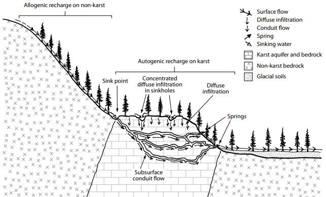
The simplest way of first classifying cave sediments is to determine whether the sediments originated inside or outside the cave. Allochthonous (or allogenic) sediments come from sources outside of the cave system and are subsequently transported underground by a variety of mechanisms such as gravity, water, wind, or animal activities (Figure 12.4.11). Autochthonous (or authigenic) sediments originate within the cave system itself. Allochthonous and autochthonous sediments can further be broken down into three sub-categories that describe their material types: clastic sediments, organic sediments, and precipitates/evaporates. Clastic sediments are the products of the mechanical breakdown of rocks. The individual particles resulting from this process are called clasts. Clastic sediments in caves can be either: allochthonous or autochthonous. A typical example of autochthonous clastic cave sediment would be large angular blocks of rock that have fallen from the cave ceiling – these are generally referred to as “breakdown”. Breakdown is often easy to identify because it is comprised of the same host bedrock as the cave and is often quite large and blocky. It is not uncommon to see breakdown blocks the size of trucks and every caver hopes not to be present in a cave when breakdown occurs. Other autochthonous cave sediments owe their origins to less dramatic events. For example, some limestone contains nodules of insoluble materials like chert. As the limestone containing these nodules dissolves around them, they are released from the bedrock and become autochthonous sediments in the cave.</p> <p>Allochthonous clastic cave sediments originate in the cave’s catchment and are transported into the cave system by water, gravity, and wind (Figure 12.4.11). Caves that were once at or below sea level may contain marine deposits carried in by wave action and tides. Allochthonous organic sediments may enter cave systems by these means as well but can also be transported in by living organisms such as bats, birds, denning animals, and humans. Human occupation of caves over long periods of time can result in surprisingly deep culturally derived sediment deposits, but these archaeologically significant deposits are usually confined to cave entrance zones which offer more favourable habitation sites than areas deeper within the caves. The activities of other animals such as bears, or bats can contribute to organic sediments in areas well beyond the entrance zones. Some of the clays and sands present in caves are produced this way.
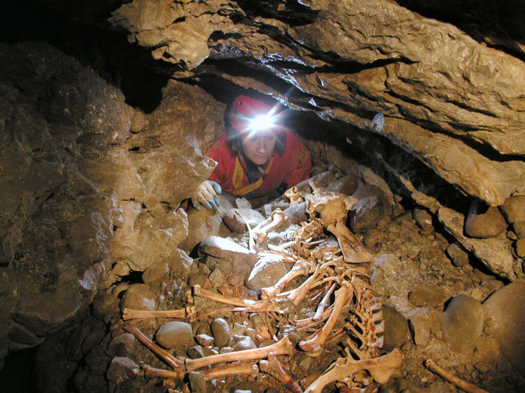
</p> <div class="wp-caption aligncenter" id="attachment_460" aria-describedby="caption-attachment-460" style="width: 718px"><a href="http://environmental-geology-dev.pressbooks.tru.ca/wp-content/uploads/sites/73/2021/07/Fig-36.jpg" data-url="http://environmental-geology-dev.pressbooks.tru.ca/wp-content/uploads/sites/73/2021/07/Fig-36.jpg"><img class="wp-image-559" src="http://environmental-geol.pressbooks.tru.ca/wp-content/uploads/sites/123/2022/08/Fig-36-1024x768.jpg" alt="" width="718" height="539" srcset="https://environmental-geol.pressbooks.tru.ca/wp-content/uploads/sites/123/2022/08/Fig-36-1024x768.jpg 1024w, https://environmental-geol.pressbooks.tru.ca/wp-content/uploads/sites/123/2022/08/Fig-36-300x225.jpg 300w, https://environmental-geol.pressbooks.tru.ca/wp-content/uploads/sites/123/2022/08/Fig-36-768x576.jpg 768w, https://environmental-geol.pressbooks.tru.ca/wp-content/uploads/sites/123/2022/08/Fig-36-65x49.jpg 65w, https://environmental-geol.pressbooks.tru.ca/wp-content/uploads/sites/123/2022/08/Fig-36-225x169.jpg 225w, https://environmental-geol.pressbooks.tru.ca/wp-content/uploads/sites/123/2022/08/Fig-36-350x263.jpg 350w, https://environmental-geol.pressbooks.tru.ca/wp-content/uploads/sites/123/2022/08/Fig-36.jpg 1501w" sizes="(max-width: 718px) 100vw, 718px" title="" /></a><div class="wp-caption-text" id="caption-attachment-460"><strong>Figure 12.4.11</strong> Deer Bones and Unconsolidated Cave Sediments</div></div> <p>Accurate interpretation of cave sediments requires familiarity with both cave processes and the principles of sedimentology, as well as access to appropriate dating techniques. The study of cave sediments can potentially yield information about events in a cave’s history but interpreting them is not always a straightforward task. Of course, this does not mean that reworked or redeposited sediments are useless or without value, as they can always tell us something about energy regimes, transport mechanisms and depositional environments within the cave. The trick is really to understand the limitations of what cave sediments can reveal and to ask the appropriate questions, based on those constraints.</p> <h1>Subterranean Life</h1> <p>At first glance, caves seem rather barren places, and inhospitable to life. In the constant darkness underground photosynthesis cannot take place, so the primary producers of surface ecosystems – living photosynthetic plants – are almost completely absent. In cave environments, the base of the food web starts with fungi and bacteria. Plant material in the form of detritus and other organic debris is transferred into caves by water, gravity, air currents and is broken down by these organisms. Animal carcasses – especially those of bats – can also be an important source of nutrients, as is bat guano. In some caves the “food delivery system” may be erratic, but even when this is not the case, productivity in cave ecosystems tends to be quite low compared with surface ecosystems.</p> <p>
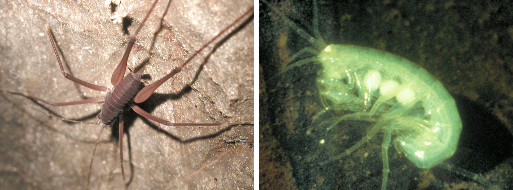
Not all cave ecosystems are based on organic substances transported in from the surface, however. In some caves – Mexico’s Cueva de Villa Luz, for example – inorganic substances like hydrogen sulfide provide the energy source for sulfur eating bacteria, which are then consumed by other organisms in the food web. Larger protozoans, beetles, snails, nematodes, flatworms, springtails, and millipedes can all function as detritovores (i.e., organisms which feed directly on organic detritus) in cave ecosystems. While smaller organisms may act as microbivores by feeding on the bacterial and fungal hyphae. These in turn may be preyed upon by fish, spiders, crustaceans, centipedes, beetles and other larger vertebrates and invertebrates in the cave (Figure 12.4.12). Some of the larger vertebrates found in caves include salamanders and bats. In cave ecosystems, species richness (or the range of different species) may be quite high, but the overall number of organisms supported may be low as compared to surface ecosystems of a similar size.</p> <div class="wp-caption aligncenter" id="attachment_461" aria-describedby="caption-attachment-461" style="width: 735px"><a href="http://environmental-geology-dev.pressbooks.tru.ca/wp-content/uploads/sites/73/2021/07/cave-life-1.jpg" data-url="http://environmental-geology-dev.pressbooks.tru.ca/wp-content/uploads/sites/73/2021/07/cave-life-1.jpg"><img class="wp-image-560" src="http://environmental-geol.pressbooks.tru.ca/wp-content/uploads/sites/123/2022/08/cave-life-1-1024x380.jpg" alt="" width="735" height="273" srcset="https://environmental-geol.pressbooks.tru.ca/wp-content/uploads/sites/123/2022/08/cave-life-1-1024x380.jpg 1024w, https://environmental-geol.pressbooks.tru.ca/wp-content/uploads/sites/123/2022/08/cave-life-1-300x111.jpg 300w, https://environmental-geol.pressbooks.tru.ca/wp-content/uploads/sites/123/2022/08/cave-life-1-768x285.jpg 768w, https://environmental-geol.pressbooks.tru.ca/wp-content/uploads/sites/123/2022/08/cave-life-1-1536x571.jpg 1536w, https://environmental-geol.pressbooks.tru.ca/wp-content/uploads/sites/123/2022/08/cave-life-1-65x24.jpg 65w, https://environmental-geol.pressbooks.tru.ca/wp-content/uploads/sites/123/2022/08/cave-life-1-225x84.jpg 225w, https://environmental-geol.pressbooks.tru.ca/wp-content/uploads/sites/123/2022/08/cave-life-1-350x130.jpg 350w, https://environmental-geol.pressbooks.tru.ca/wp-content/uploads/sites/123/2022/08/cave-life-1.jpg 1771w" sizes="(max-width: 735px) 100vw, 735px" title="" /></a><div class="wp-caption-text" id="caption-attachment-461"><strong>Figure 12.4.12</strong> Cave Cricket (left), and Cave Amphipod (right)</div></div> <p>In cave-adapted organisms, eyes are often rudimentary structures, or totally absent. By contrast, their other sensory organs may be highly specialized and enlarged. They tend to lack pigmentation, and their appendages (if they have any) may be modified to give them better purchase on rocky wall and floors. They may have different cycles of activity than those of surface dwellers. Finally, they tend to be small, and have lower metabolic rates. Remember, photosynthesis cannot occur in caves, so the food web is mostly based on meager supplies of available nutrients (perhaps in the form of organic detritus or guano) transported into the cave, either by water, gravity, air currents, or other animals. In any case, productivity is relatively low – so there are advantages to being small, fuel efficient, and not too prolific.</p> <p>Subterranean life forms are classified according to how dependent they are on the underground environment. Troglobites are cave-adapted organisms that cannot survive on the surface and must spend their entire lives in caves. Troglophiles are creatures that can spend their entire lives in caves, but that also occur in similar dark, damp surface environments. These include species of spiders, crickets, and salamanders. Trogloxenes are organisms that use caves for some portion of their life cycle, but that also spend part of their time on the surface including bats and harvestman, both of which forage outside of caves. Accidentals are creatures have no special affinity for caves; instead, they have either wandered in under their own power or ended up there by accident – by falling down a shaft, say, or being washed in. Extremophiles are not necessarily cave-dwelling organisms and refers to organisms that have adapted to conditions such as temperature, pH, or the mixture of atmospheric gasses that fall outside what we humans consider to be outside the normal range. Extremophiles are microbes that have been found living in or around extreme environments such as undersea hot vents but can also occur in some caves.</p> <h3><strong>Media Attributions</strong></h3> <ul><li><strong>Figure 12.4.1</strong> Photo by T. Stokes, <a href="https://creativecommons.org/licenses/by/4.0/" data-url="https://creativecommons.org/licenses/by/4.0/">CC BY 4.0</a></li> <li><strong>Figure 12.4.2&nbsp;</strong>Photo by Steven Earle, <a href="https://creativecommons.org/licenses/by/4.0/" data-url="https://creativecommons.org/licenses/by/4.0/">CC BY 4.0</a></li> <li><strong>Figure 12.4.3&nbsp;</strong>Photo by P. Griffiths, <a href="https://creativecommons.org/licenses/by/4.0/" data-url="https://creativecommons.org/licenses/by/4.0/">CC BY 4.0</a></li> <li><strong>Figure 12.4.4 </strong>Photo by P. Griffiths, <a href="https://creativecommons.org/licenses/by/4.0/" data-url="https://creativecommons.org/licenses/by/4.0/">CC BY 4.0</a></li> <li><strong>Figure 12.4.5 </strong>Photo by P. Griffiths, <a href="https://creativecommons.org/licenses/by/4.0/" data-url="https://creativecommons.org/licenses/by/4.0/">CC BY 4.0</a></li> <li><strong>Figure 12.4.6 </strong>Photo by P. Griffiths, <a href="https://creativecommons.org/licenses/by/4.0/" data-url="https://creativecommons.org/licenses/by/4.0/">CC BY 4.0</a></li> <li><strong>Figure 12.4.7 </strong>Photo by P. Griffiths, <a href="https://creativecommons.org/licenses/by/4.0/" data-url="https://creativecommons.org/licenses/by/4.0/">CC BY 4.0</a></li> <li><strong>Figure 12.4.8 </strong>Photos by P. Griffiths, <a href="https://creativecommons.org/licenses/by/4.0/" data-url="https://creativecommons.org/licenses/by/4.0/">CC BY 4.0</a></li> <li><strong>Figure 12.4.9 </strong>Photo by T. Stokes, <a href="https://creativecommons.org/licenses/by/4.0/" data-url="https://creativecommons.org/licenses/by/4.0/">CC BY 4.0</a></li> <li><strong>Figure 12.4.10 </strong><a href="https://www.piqsels.com/en/public-domain-photo-zibbt/" data-url="https://www.piqsels.com/en/public-domain-photo-zibbt/">Photo</a> is <a href="https://www.piqsels.com/terms-of-service" data-url="https://www.piqsels.com/terms-of-service">Public domain</a> from Piqsels.com, https://www.piqsels.com/en/public-domain-photo-zibbt/</li> <li><strong>Figure 12.4.11 </strong>Photo by P. Griffiths, <a href="https://creativecommons.org/licenses/by/4.0/" data-url="https://creativecommons.org/licenses/by/4.0/">CC BY 4.0</a></li> <li><strong>Figure 12.4.12 </strong>Photos by P. Griffiths, <a href="https://creativecommons.org/licenses/by/4.0/" data-url="https://creativecommons.org/licenses/by/4.0/">CC BY 4.0</a></li> </ul> 
	</div>


	</div>
<div class="chapter standard " id="chapter-origin-and-genesis-of-caves" title="12.5 Origin and Genesis of Caves">
	<div class="chapter-title-wrap">
		<p class="chapter-number">71</p>
		<h1 class="chapter-title">12.5 Origin and Genesis of Caves</h1>
					<p class="chapter-author">Steve Earle</p>
			</div>
	<div class="ugc chapter-ugc">
				 <p>The origin and genesis of karst caves has been a hotly debated subject in both geological and speleological circles for centuries. Are caves formed above the water table (vadose conditions), below the water table (phreatic conditions), along the water table (hypophreatic), from hydrothermal water sources or by some other processes?</p> <p>More recently there appears to be some consensus to this question – not always the way in science! Approximately 90% of known karst caves are thought to have formed from meteoric water sources (i.e., from water that has originated from the surface.) A small percentage of caves have formed by warm hydrothermal solutions emanating from deeper sources in the Earth (such as from a slow cooling granitic body), with H<sub>2</sub>S mainly being responsible for making the acidic waters available for bedrock dissolution. This is known a hypogenic karst.</p> <p>The generally accepted hypothesis for karst cave genesis is as follows. Meteoric water falling or flowing onto the karst landscape infiltrates the ground surface and percolates through the vadose zone down to the water table – below which all cavities are filled with water. Water in the phreatic zone, below the water table, flows slowly towards an output, such as a spring at a topographic low. As this water flows from the input to output sites it creates a U-shaped conduit known as a ‘phreatic loop’, which extends for some distance underground. The depth of this loop is dependent on the orientation of primary structures within the bedrock (e.g., bedding planes and joints) and the distance between the sites of water input and output. The greater the distance between input and output and the steeper the bedding planes, the deeper the phreatic loop. (Trying to fully prove this concept by direct observation moves into the realm of cave diving—a highly skilled and hazardous research technique!) Most caves are thought to have initially formed in this way with the phreatic loop forming a trunk or main passage for the cave. Other side passages can form above, below and along the sides of this preferred loop, and may link up with other main passages.</p> <p>The landscape and the associated water table is likely to fall or rise over time, possibly due to changes in sea level and/or tectonic uplift or subsidence. This has a major effect on the cave formation process. If the water table rises (e.g., if the ground subsides, or the sea level rises) the locations of water input and output will change. Solution process along the phreatic loop will cease as water flow will become very slow or stationary.</p> <p>Caves above the phreatic zone, if any, will become water-filled and used as preferential sites for water flow (i.e., the vadose cave system will become reactivated). On the other hand, if the water table is lowered as the landscape becomes uplifted, a new deeper phreatic loop will develop, while the older phreatic loop will become partially air-filled (vadose) with a stream channel along the floor of the passage. This stream channel will flow faster and likely contain coarse clastic sediments that will erode and cut into the phreatic tube, and possibly form a small slot, such as a keyhole passage. Sediments could also be moved and redeposited, and seepage/drips would form speleothems on the ceiling and walls. As the new phreatic loop continues to develop below the vadose passage it could potentially capture the stream above and lead to ‘drying’ of the vadose passage. As might be anticipated with continental tectonic uplift and dissolution, a multi-level cave system could develop. However, over long geologic periods this can be complicated by changes in climate (e.g., ice ages, glaciation, and de-glaciation), as well as the rates of tectonic movements. Some of these processes are illustrated on Figure 12.5.1.</p> <p>This well accepted model of multi-level cave development by Ewers and Ford (1978)<span class="footnote"><span class="footnote-indirect" data-fnref="564-1"></span></span> is based on the premise of a lowering base level (water table) over time, which might occur during the incision of a major river valley, tectonic uplift, or by changes in sea level. The model demonstrates a gradual increase in the frequency of enlarged fractures or fissures (black lines) during the dissolution of carbonate bedrock by infiltrating water that moves from the surface to output sites (on the left side of images). These output sites might occur as karst springs near a valley bottom. In b) a water filled conduit (solid blue lines) develops along a phreatic loop as fissures become enlarged and forming a cave in c) connecting input and output sites. As the base level lowers in d) and e) a second phreatic loop develops along the new water table, leaving the upper cave air filled (open blue lines) and in the vadose zone. With final lowering of base level in f) a third phreatic loop develops near the water table abandoning the previous two loops and caves above and leaving them both in the vadose zone.</p> <div class="wp-caption aligncenter" id="attachment_463" aria-describedby="caption-attachment-463" style="width: 734px"><a href="http://environmental-geology-dev.pressbooks.tru.ca/wp-content/uploads/sites/73/2021/07/karst-evolution.jpg" data-url="http://environmental-geology-dev.pressbooks.tru.ca/wp-content/uploads/sites/73/2021/07/karst-evolution.jpg"><img class="wp-image-563" src="http://environmental-geol.pressbooks.tru.ca/wp-content/uploads/sites/123/2021/07/karst-evolution-1024x531.jpg" alt="" width="734" height="381" srcset="https://environmental-geol.pressbooks.tru.ca/wp-content/uploads/sites/123/2021/07/karst-evolution-1024x531.jpg 1024w, https://environmental-geol.pressbooks.tru.ca/wp-content/uploads/sites/123/2021/07/karst-evolution-300x155.jpg 300w, https://environmental-geol.pressbooks.tru.ca/wp-content/uploads/sites/123/2021/07/karst-evolution-768x398.jpg 768w, https://environmental-geol.pressbooks.tru.ca/wp-content/uploads/sites/123/2021/07/karst-evolution-1536x796.jpg 1536w, https://environmental-geol.pressbooks.tru.ca/wp-content/uploads/sites/123/2021/07/karst-evolution-65x34.jpg 65w, https://environmental-geol.pressbooks.tru.ca/wp-content/uploads/sites/123/2021/07/karst-evolution-225x117.jpg 225w, https://environmental-geol.pressbooks.tru.ca/wp-content/uploads/sites/123/2021/07/karst-evolution-350x181.jpg 350w, https://environmental-geol.pressbooks.tru.ca/wp-content/uploads/sites/123/2021/07/karst-evolution.jpg 1582w" sizes="(max-width: 734px) 100vw, 734px" title="" /></a><div class="wp-caption-text" id="caption-attachment-463"><strong>Figure 12.5.1</strong> Formation of Phreatic Loop and Cave Genesis Under a Falling Water Table</div></div> <p>The time of inception to the end of cave formation is not clearly defined. However, the answer is in part linked rates of erosion, and denudation of karst landscapes. Most of the research suggests that 3000-5000 years is required for a proto-cave 5-15 mm in size to develop, and 5000-100,000 years is required to form an opening 1-10 m or more.<span class="footnote"><span class="footnote-indirect" data-fnref="564-2"></span></span> This is of course speculative and depends on the continuity of the solution process and many other possible variables (e.g., climate, tectonic uplift, and glaciation). A variety of analytical techniques can be used to directly date materials found in a cave. Fossils in cave sediments can be dated using <sup>14</sup>C and speleothems can be dated using <sup>234</sup>U-<sup>230</sup>Th techniques. This information can place constraints on the time for cave formation. For example, speleothems from Castleguard Cave (the longest known cave in Canada, located along the BC-Alberta border) were dated at 780,000 years, indicating that the main episode of cave development liked ended at or near this time, and the passages probably formed many thousands of years earlier. On Vancouver Island speleothems have been dated at 15,000 – 18,500 years, suggesting caves could be of younger origin.<span class="footnote"><span class="footnote-indirect" data-fnref="564-3"></span></span>.</p> <p>Studies from south-east Australia suggest that some caves in that region are in the order of 300 million years old.<span class="footnote"><span class="footnote-indirect" data-fnref="564-4"></span></span>. If this is correct, we could, when entering these caves, be going into environments that have been basically unchanged for vast periods of geologic time. Overall, the determination of a cave’s age is not clear cut, particularly when it is difficult to construe when cave development begins and when it ends. It is quite possible for old cave passages to be uplifted and ‘dried out’, then submerged, re-developed, and then uplifted again. The only sure end to cave development is when it is uplifted and totally eroded away!</p> <h3><strong>Media Attribution</strong></h3> <ul><li><strong>Figure 12.5.1</strong> Steven Earle, <a href="https://creativecommons.org/licenses/by/4.0/" data-url="https://creativecommons.org/licenses/by/4.0/">CC BY 4.0</a>, after Ford and Ewers (1978)</li> </ul> <p>&nbsp;</p> 
	</div>
			
				
				<div class="footnotes"><div id='564-1'>Ford, D. and Ewers, R. (1978). The development of limestone cave systems in the dimensions of length and depth. International Journal of Speleology, 10: 213-244. http://dx.doi.org/10.5038/1827-806X.10.3.1</div><div id='564-2'>White, B. (1988). <em>Geomorphology and hydrology of karst terrains.</em> Oxford University Press.</div><div id='564-3'>Stokes, T. R., &amp; Griffiths, P. A. (2019). An Overview of the Karst Areas in British Columbia, Canada. <em>Geoscience Canada, 46</em>(1), 49–66. https://doi.org/10.12789/geocanj.2019.46.145</div><div id='564-4'>Armstrong, O. (2003). The world’s oldest cave – how did they survive and what can they tell us? <em>Acta Carsologica, 36</em>(1), 134–142. https://doi.org/10.3986/ac.v36i1.215</div></div>
	</div>
<div class="chapter standard " id="chapter-human-interactions-with-karst-and-caves" title="12.6 Human Interactions with Karst and Caves">
	<div class="chapter-title-wrap">
		<p class="chapter-number">72</p>
		<h1 class="chapter-title">12.6 Human Interactions with Karst and Caves</h1>
					<p class="chapter-author">Steve Earle</p>
			</div>
	<div class="ugc chapter-ugc">
				 <p>Human interactions with karst and caves have ranged from the sacred to the profane. Many karst features like cave entrance and springs have always served as natural focal points for human activities by providing two of life’s most necessities – shelter and water. Karst caves have been used as shelters by humans on every continent throughout human history. For example, Tabun Cave, near Mt. Carmel, Israel, shows evidence for periodic human/hominid occupation between 40,000 to half a million years ago.<span class="footnote"><span class="footnote-indirect" data-fnref="572-1"></span></span> Humans have continued to use caves for various purposes throughout history right up to the present day. They have been utilized for the storage of Roquefort cheese in France, as root cellars and storage of canned goods, milk, and whiskey in Kentucky, and as fuel caches by the Nazis in Slovenia (Figure 12.6.1). Caves were sometimes used as air raid shelters in Europe during World War II and have more recently been considered as potential nuclear fallout shelters. In Turkey and Hungary, cave sanatoria have been established to provide respiratory therapy for such conditions as bronchial asthma. Cave discotheques exist today in China and Cuba for those with entertainment in mind. As well, underground symphonies and musical concerts have been performed in several countries. Those more interested in extreme sports may be gratified to learn that underground hot air balloon expeditions have been undertaken in French and American caves in recent years.</p> <div class="wp-caption aligncenter" id="attachment_836" aria-describedby="caption-attachment-836" style="width: 600px"><a href="http://environmental-geology-dev.pressbooks.tru.ca/wp-content/uploads/sites/73/2021/07/Fig-41-scaled-1.jpg" data-url="http://environmental-geology-dev.pressbooks.tru.ca/wp-content/uploads/sites/73/2021/07/Fig-41-scaled-1.jpg"><img class="wp-image-566" src="http://environmental-geol.pressbooks.tru.ca/wp-content/uploads/sites/123/2021/07/Fig-41-scaled-1.jpg" alt="" width="600" height="451" srcset="https://environmental-geol.pressbooks.tru.ca/wp-content/uploads/sites/123/2021/07/Fig-41-scaled-1.jpg 2560w, https://environmental-geol.pressbooks.tru.ca/wp-content/uploads/sites/123/2021/07/Fig-41-scaled-1-300x225.jpg 300w, https://environmental-geol.pressbooks.tru.ca/wp-content/uploads/sites/123/2021/07/Fig-41-scaled-1-1024x768.jpg 1024w, https://environmental-geol.pressbooks.tru.ca/wp-content/uploads/sites/123/2021/07/Fig-41-scaled-1-768x576.jpg 768w, https://environmental-geol.pressbooks.tru.ca/wp-content/uploads/sites/123/2021/07/Fig-41-scaled-1-1536x1153.jpg 1536w, https://environmental-geol.pressbooks.tru.ca/wp-content/uploads/sites/123/2021/07/Fig-41-scaled-1-2048x1537.jpg 2048w, https://environmental-geol.pressbooks.tru.ca/wp-content/uploads/sites/123/2021/07/Fig-41-scaled-1-65x49.jpg 65w, https://environmental-geol.pressbooks.tru.ca/wp-content/uploads/sites/123/2021/07/Fig-41-scaled-1-225x169.jpg 225w, https://environmental-geol.pressbooks.tru.ca/wp-content/uploads/sites/123/2021/07/Fig-41-scaled-1-350x263.jpg 350w" sizes="(max-width: 600px) 100vw, 600px" title="" /></a><div class="wp-caption-text" id="caption-attachment-836"><strong>Figure 12.6.1</strong> A Restaurant in the Entrance to Lost River Cave, Bowling Green, Kentucky</div></div> <p>Subterranean drainage is one of the defining characteristics of well-developed karst landscapes. For this reason, knowledge of the locations of karst springs has been essential to humans inhabiting such regions in the past (Figure 12.6.2). For example, in Mexico’s Yucatan Peninsula. This huge limestone plateau, which has neither large lakes nor rivers flowing over the surface, supported the development and flowering of the Mayan civilization in pre-Hispanic times. Archaeological evidence suggests that though the Maya utilized water from cenotes and underground rivers for practical purposes, these karst features also played an important role in their religious rituals and beliefs. The use of caves as shrines, temples, or spaces for ritual activities has been widespread through human history, including Minoan sites in Crete, the Mayan caves, and cenotes in the Yucatan, and in various places in Asia. A small cave in Bocas del Toro, Panama, serves as a shrine and outdoor chapel today; it is also a pilgrimage site for Catholics, as is the much more famous Grotto at Lourdes.</p> <div class="wp-caption aligncenter" id="attachment_837" aria-describedby="caption-attachment-837" style="width: 602px"><a href="http://environmental-geology-dev.pressbooks.tru.ca/wp-content/uploads/sites/73/2021/07/Fig-42.jpeg" data-url="http://environmental-geology-dev.pressbooks.tru.ca/wp-content/uploads/sites/73/2021/07/Fig-42.jpeg"><img class="wp-image-567" src="http://environmental-geol.pressbooks.tru.ca/wp-content/uploads/sites/123/2022/08/Fig-42.jpeg" alt="" width="602" height="451" srcset="https://environmental-geol.pressbooks.tru.ca/wp-content/uploads/sites/123/2022/08/Fig-42.jpeg 1967w, https://environmental-geol.pressbooks.tru.ca/wp-content/uploads/sites/123/2022/08/Fig-42-300x225.jpeg 300w, https://environmental-geol.pressbooks.tru.ca/wp-content/uploads/sites/123/2022/08/Fig-42-1024x768.jpeg 1024w, https://environmental-geol.pressbooks.tru.ca/wp-content/uploads/sites/123/2022/08/Fig-42-768x576.jpeg 768w, https://environmental-geol.pressbooks.tru.ca/wp-content/uploads/sites/123/2022/08/Fig-42-1536x1152.jpeg 1536w, https://environmental-geol.pressbooks.tru.ca/wp-content/uploads/sites/123/2022/08/Fig-42-65x49.jpeg 65w, https://environmental-geol.pressbooks.tru.ca/wp-content/uploads/sites/123/2022/08/Fig-42-225x169.jpeg 225w, https://environmental-geol.pressbooks.tru.ca/wp-content/uploads/sites/123/2022/08/Fig-42-350x262.jpeg 350w" sizes="(max-width: 602px) 100vw, 602px" title="" /></a><div class="wp-caption-text" id="caption-attachment-837"><strong>Figure 12.6.2</strong> The ‘Fluerette’ Fountain Emerging from a Karst Spring, Nerac, Southern France</div></div> <p>Many cultures have used karst features such as caves and sinkholes for more detrimental purposes. Dumping refuse in caves and sinkholes—a practice that can have negative implications on conservation—is still a relatively common practice in some parts of the world. The use of caves as places of internment for human remains has been quite common in some cultures in the past. People have also ventured into caves in search of various economic resources. For example, swift nests, the namesake ingredient in Bird’s Nest soup, have been harvested from caves on Thailand’s Phangnga archipelago for hundreds of years. This practice continues today.</p> <h1>Cave Conservation, Show Caves and Karst Parks</h1> <p>Caves—or some parts of caves—can be particularly vulnerable to disturbances caused by human visitors (Figure 12.6.3). Every trip underground entails some impact to the cave environment. Even by sitting motionless in an underground cavern, a single human is subtly altering the underground ecosystem. He or she is exhaling carbon dioxide, radiating body heat, introducing light and noise, shedding skin cells and hair, and transporting dirt or other foreign substances on his or her clothing and shoes. The cumulative effects of such subtle impacts can present real challenges to cave managers in popular show caves. Perhaps the single biggest conservation concern in caves revolves around preserving speleothems such as stalactites, draperies, and flowstone. Many of these calcite formations are very fragile and have taken hundreds or thousands of years to form. They can be broken by careless handling or soiled by contact with dirty clothing, boots, or hands. The best way to preserve such formations is to stay away from them altogether.</p> <div class="wp-caption aligncenter" id="attachment_838" aria-describedby="caption-attachment-838" style="width: 598px"><a href="http://environmental-geology-dev.pressbooks.tru.ca/wp-content/uploads/sites/73/2021/07/Fig-43-scaled-1.jpg" data-url="http://environmental-geology-dev.pressbooks.tru.ca/wp-content/uploads/sites/73/2021/07/Fig-43-scaled-1.jpg"><img class="wp-image-568" src="http://environmental-geol.pressbooks.tru.ca/wp-content/uploads/sites/123/2022/08/Fig-43-scaled-1.jpg" alt="" width="598" height="798" srcset="https://environmental-geol.pressbooks.tru.ca/wp-content/uploads/sites/123/2022/08/Fig-43-scaled-1.jpg 1920w, https://environmental-geol.pressbooks.tru.ca/wp-content/uploads/sites/123/2022/08/Fig-43-scaled-1-225x300.jpg 225w, https://environmental-geol.pressbooks.tru.ca/wp-content/uploads/sites/123/2022/08/Fig-43-scaled-1-768x1024.jpg 768w, https://environmental-geol.pressbooks.tru.ca/wp-content/uploads/sites/123/2022/08/Fig-43-scaled-1-1152x1536.jpg 1152w, https://environmental-geol.pressbooks.tru.ca/wp-content/uploads/sites/123/2022/08/Fig-43-scaled-1-1536x2048.jpg 1536w, https://environmental-geol.pressbooks.tru.ca/wp-content/uploads/sites/123/2022/08/Fig-43-scaled-1-65x87.jpg 65w, https://environmental-geol.pressbooks.tru.ca/wp-content/uploads/sites/123/2022/08/Fig-43-scaled-1-350x467.jpg 350w" sizes="(max-width: 598px) 100vw, 598px" title="" /></a><div class="wp-caption-text" id="caption-attachment-838"><strong>Figure 12.6.3</strong> Guided Tour in Progress at Mammoth Caves National Park, Kentucky</div></div> <p>Conservation-oriented caving involves minimizing any trace of human intrusion in the underground environment, so that others may also enjoy it in its pristine state. Most cavers adhere to a Caving Code of Ethics.<span class="footnote"><span class="footnote-indirect" data-fnref="572-2"></span></span> Though these codes may vary somewhat in their wording, they can generally be summarized in the motto, “Take nothing but pictures; leave nothing but footprints”. Some cavers would argue that even leaving footprints constitutes an unacceptable human impact underground, and subscribe to the more demanding creed, “Leave no trace”. Because it is almost impossible for humans to leave no trace, particularly in low-energy parts of a cave, strict adherence to this creed sometimes requires that one refrain from entering such areas altogether.</p> <p>A show cave is a cave that has been developed to facilitate access and viewing by visitors without the need for special equipment or skills. Show caves are often fitted with walkways, stairs, and lighting systems. Guides are frequently available to accompany groups of paying visitors, providing interpretation, and pointing out features of interest. The advantages of visiting show caves are that they are safely and easily accessible to most people, they are frequently very beautiful, interpretation is provided, and no special equipment, athletic prowess, or technical skills are needed to get in. Controlling the effects of infrastructure (such as walkways and lights) as well as impacts caused by large numbers of visitors passing through show caves can present real challenges to managers.</p> <p>People usually have several options for viewing caves and karst in many regions of the world. On Vancouver Island there are cave and karst areas such as the Horne Lake Caves Provincial Park or Upana Caves, where people have access to self-guided and guided tours through safe, easily accessible wild caves as well as nature walks in typical west coast forested karst. People with sufficient funds can sign up for ecotours which include cave and karst viewing in more exotic locals such as Madagascar, Thailand, or Belize. Many countries such as France, Australia, the USA, and Slovenia have extensive karst that people can view or visit as they tour about on their own. Prince of Wales Island, Alaska, has an excellent infrastructure for self-guided karst viewing.</p> <h1>The Economic Values of Karst</h1> <p>Karst aquifers are of particular importance as sources of water for drinking, domestic use, and irrigation in regions where little surface drainage exists. Some bottled waters such as Evian (and Perrier) are obtained from karst springs and are especially valued by for their mineral content. Palaeokarst (karst that formed in the past and is preserved in the geologic record) can also serve as important reservoirs for oil and natural gas. Examples of these types of reservoirs are found in many parts of western Canada’s oilfields, such as the Leduc Formation.</p> <p>One thing that the economic values listed above have in common is that all are based on resource extraction from karst. Resource extraction can have significant impact on many components of the karst system. It is also important to consider the non-extractive economic values of karst as well. For example, one non-extractive value pertains to a link between karst and fisheries. Alaskan research suggests that karst aquatic systems can be up to ten times more productive than non-karst systems, and possess various other qualities thought to boost fish productivity.</p> <p>Today, the tourism and recreational potential of karst is increasingly recognized in many countries and may provide a sustainable alternative to resource extraction or an entirely new economic opportunity. Some karst has been popular with sightseers for centuries – the tower karst of Guilin, China, being an obvious example (Figure 12.2.2). Adventurous ecotourists today can go cave diving in cenotes of Belize and other parts of the Yucatan Peninsula, or visit the spectacular caves and limestone spires of Madagascar’s Tsingy de Bemaraha Park. In the long run, the trend toward interpretive ecotourism may raise public awareness as to the natural values of karst, and thus be beneficial for karst conservation efforts.</p> <h1>Agriculture and Forestry on Karst</h1> <p>Many agricultural practices involve clearing natural vegetation – either for crop cultivation or through grazing by domesticated herd animals. Disturbing the natural vegetation cover can alter water budgets in karst systems. Tillage can also disturb soils, leading to greater rates of erosion and subsequent increases if sediment moves into subsurface waterways. Agricultural chemicals such a herbicides, insecticides and fertilizers that are spread on karst lands as they can infiltrate into underlying karst aquifers. Likewise for animal waste products (e.g., effluents from manure lagoons) that enter karst hydrological systems and artificially alter subterranean nutrient balances and subsequently contaminate the water.</p> <p>Forestry activities on karst can inadvertently lead to the disruption of shallow caves, the redirection of water flow during forest road construction, logging near sensitive features (e.g., large sinkholes) and the loss of soil into vertical solutional openings or epikarst. Fires can also be problematic on karst (Figure 12.6.5). Intense fires, such as those that occur when burning logging slash piles within a forestry cut block can destroy organic components in soil as well as root systems that hold the soil in place. On thinly soiled epikarst, such fires can result in soil loss through incineration and erosion, thus slowing or hampering the regeneration of the vegetation cover and new tree growth. Less intensive fires may not damage the soil cover on karst, but the burning regimen can still alter regrowth by favouring the survival of more fire-tolerant species. In BC there is a comprehensive set of inventory procedures and management guidelines for forestry operations on karst.<span class="footnote"><span class="footnote-indirect" data-fnref="572-3"></span></span> The intent of these guidelines is to use an ecosystem-based or catchment-based approach, rather than focusing on the management of individual karst features or caves.</p> <div class="wp-caption aligncenter" id="attachment_469" aria-describedby="caption-attachment-469" style="width: 732px"><a href="http://environmental-geology-dev.pressbooks.tru.ca/wp-content/uploads/sites/73/2021/07/Fig-48.jpg" data-url="http://environmental-geology-dev.pressbooks.tru.ca/wp-content/uploads/sites/73/2021/07/Fig-48.jpg"><img class="wp-image-569" src="http://environmental-geol.pressbooks.tru.ca/wp-content/uploads/sites/123/2022/08/Fig-48-1024x768.jpg" alt="" width="732" height="548" srcset="https://environmental-geol.pressbooks.tru.ca/wp-content/uploads/sites/123/2022/08/Fig-48-1024x768.jpg 1024w, https://environmental-geol.pressbooks.tru.ca/wp-content/uploads/sites/123/2022/08/Fig-48-300x225.jpg 300w, https://environmental-geol.pressbooks.tru.ca/wp-content/uploads/sites/123/2022/08/Fig-48-768x576.jpg 768w, https://environmental-geol.pressbooks.tru.ca/wp-content/uploads/sites/123/2022/08/Fig-48-65x49.jpg 65w, https://environmental-geol.pressbooks.tru.ca/wp-content/uploads/sites/123/2022/08/Fig-48-225x169.jpg 225w, https://environmental-geol.pressbooks.tru.ca/wp-content/uploads/sites/123/2022/08/Fig-48-350x263.jpg 350w, https://environmental-geol.pressbooks.tru.ca/wp-content/uploads/sites/123/2022/08/Fig-48.jpg 1501w" sizes="(max-width: 732px) 100vw, 732px" title="" /></a><div class="wp-caption-text" id="caption-attachment-469"><strong>Figure 12.6.4</strong> Tree Removal and Burning are Leading to Increased Soil Loss in Exposed Epikarst Areas, Northern Vancouver Island</div></div> <h1>Engineering Projects on Karst</h1> <p>Karst terrain represents probably the most demanding environment for engineering projects due to its inherent variability and unpredictability. Investigations are required to reduce the primary hazards of ground instability and water infiltration, using techniques such as mapping, drilling of boreholes and geophysics. These techniques aid in locating underground cavities, assessing subsidence or sinkhole hazards, and evaluating underground water flow. Dams and reservoirs can be constructed on karst but factors such as the foundation stability and seepage beneath the reservoir, dam, and its side slopes (or abutments) needed to be considered along with mitigation techniques (e.g., grout curtains). Leakage may occur through fissures, caves, and conduits if they are not recognized and remediated. Tunneling projects in karst are of concern with groundwater being the principal hazard with the potential for rapid flooding and sediment inrushes (a major safety concern) and instability of the tunnel roof and walls. Dewatering of the overlying karst can also have significant environmental impacts ranging from declining yields in water wells and springs to sudden development of sinkholes.</p> <p>Highways can be affected by subsidence and collapse of sinkholes – the result of foundation issues or redirecting storm water and surface runoff into soil cover above sinkholes. Pollution of groundwater due to surface runoff from roads must also be considered. Bridge abutments founded on karst should only be constructed after detailed site investigation to prove the foundations are located on sound bedrock. This may require the use of long concrete cylinders or “piles”. The foundations for buildings on karst require considerable knowledge of the subsurface karst. Grouting with concrete can be used to infill openings or they could be “bridged” with a concrete slab or raft. Good drainage control is required to avoid ground disturbance after construction. Due to the variability and high permeability of karst limestone through fissures, caves and conduits, the siting of landfill and waste dumps in these areas should be avoid. In all other above cases consideration should be given to the subsurface ecology, in some cases this aspect is forgotten. Quarries into karst bedrock need to consider the potential hazards from: flooding due to intersecting openings with high groundwater, dewatering which may lead to sinkholes and damage to structures outside the quarry property, and the stability of the excavated slopes that is controlled by both rock structures and groundwater under pressure. In some cases, engineering projects may mistakenly overlook the ecological values of karst such as associated with subsurface fauna.</p> <h1>Managing Karst Landscapes as Systems</h1> <p>All land development activities of karst areas required careful management for many reasons. At their outset, many surface development activities often entail clearing vegetation which is part of the karst system and intercepts rainfall and moderates the temperature of soils. On thinly soiled karst, removing vegetation can alter the amount of water percolating down into the subsurface, and it can also destabilize soils, resulting in increased erosion and the movement of sediments into subsurface cavities. Such sediments can choke underground water conduits in karst and redirect flows in unpredictable ways or cause back flooding, as well as damage sensitive cave resources (e.g., speleothems) (Figure 12.6.6). Road building can alter karst hydrology by impeding permeability in some areas and concentrating surface drainage in others. Moreover, runoff from these surfaces (especially in urban areas) can rapidly transport pollutants directly into subsurface watercourses. Other potential point sources of pollutants associated with land development on karst include sewage systems and landfill sites which not only have the potential to harm underground ecosystems, but also pose serious problems for surface-dwelling humans. Water carrying contaminants and pollutants introduced at one point can therefore be quickly transported far from the original sources with little opportunity for dilution. Surface development can also lead to increased demands for water. If increased demands for water results in too much water being withdrawn from karst systems, the hydrostatic pressure in underground void spaces may be decreased leading to collapse, resulting in serious damage to property and in some cases loss of life.</p> <div class="wp-caption aligncenter" id="attachment_470" aria-describedby="caption-attachment-470" style="width: 732px"><a href="http://environmental-geology-dev.pressbooks.tru.ca/wp-content/uploads/sites/73/2021/07/Fig-50.jpg" data-url="http://environmental-geology-dev.pressbooks.tru.ca/wp-content/uploads/sites/73/2021/07/Fig-50.jpg"><img class="wp-image-570" src="http://environmental-geol.pressbooks.tru.ca/wp-content/uploads/sites/123/2022/08/Fig-50-1024x768.jpg" alt="" width="732" height="550" srcset="https://environmental-geol.pressbooks.tru.ca/wp-content/uploads/sites/123/2022/08/Fig-50-1024x768.jpg 1024w, https://environmental-geol.pressbooks.tru.ca/wp-content/uploads/sites/123/2022/08/Fig-50-300x225.jpg 300w, https://environmental-geol.pressbooks.tru.ca/wp-content/uploads/sites/123/2022/08/Fig-50-768x576.jpg 768w, https://environmental-geol.pressbooks.tru.ca/wp-content/uploads/sites/123/2022/08/Fig-50-65x49.jpg 65w, https://environmental-geol.pressbooks.tru.ca/wp-content/uploads/sites/123/2022/08/Fig-50-225x169.jpg 225w, https://environmental-geol.pressbooks.tru.ca/wp-content/uploads/sites/123/2022/08/Fig-50-350x263.jpg 350w, https://environmental-geol.pressbooks.tru.ca/wp-content/uploads/sites/123/2022/08/Fig-50.jpg 1501w" sizes="(max-width: 732px) 100vw, 732px" title="" /></a><div class="wp-caption-text" id="caption-attachment-470"><strong>Figure 12.6.5</strong> Redirection of Water Drainage on Karst Leading to Subsidence and Collapse of Road Fill Material, Southeast Alaska</div></div> <p>In conclusion, karst land management requires a cooperative, holistic approach in which all values (karst and non-karst) within a contributing hydrogeologic catchment need to be considered and addressed using policies and guidelines previously agreed upon by the various interested groups or stakeholders. This approach makes particularly good sense in karst catchments, because effective surface management will cater for all the interconnected values that make up the karst system: soil, bedrock, vegetation, water, biota, and air.</p> <div class="textbox textbox--exercises"><div class="textbox__header"><p class="textbox__title">Exercise 12.4 Explore a Cave Near You</p> </div> <div class="textbox__content"><div class="wp-caption alignright" id="attachment_878" aria-describedby="caption-attachment-878" style="width: 369px"><a href="http://environmental-geology-dev.pressbooks.tru.ca/wp-content/uploads/sites/73/2021/07/horne-scaled-1.jpg" data-url="http://environmental-geology-dev.pressbooks.tru.ca/wp-content/uploads/sites/73/2021/07/horne-scaled-1.jpg"><img class="wp-image-571" src="http://environmental-geol.pressbooks.tru.ca/wp-content/uploads/sites/123/2022/08/horne-scaled-1.jpg" alt="" width="369" height="277" srcset="https://environmental-geol.pressbooks.tru.ca/wp-content/uploads/sites/123/2022/08/horne-scaled-1.jpg 2560w, https://environmental-geol.pressbooks.tru.ca/wp-content/uploads/sites/123/2022/08/horne-scaled-1-300x225.jpg 300w, https://environmental-geol.pressbooks.tru.ca/wp-content/uploads/sites/123/2022/08/horne-scaled-1-1024x768.jpg 1024w, https://environmental-geol.pressbooks.tru.ca/wp-content/uploads/sites/123/2022/08/horne-scaled-1-768x576.jpg 768w, https://environmental-geol.pressbooks.tru.ca/wp-content/uploads/sites/123/2022/08/horne-scaled-1-1536x1152.jpg 1536w, https://environmental-geol.pressbooks.tru.ca/wp-content/uploads/sites/123/2022/08/horne-scaled-1-2048x1536.jpg 2048w, https://environmental-geol.pressbooks.tru.ca/wp-content/uploads/sites/123/2022/08/horne-scaled-1-65x49.jpg 65w, https://environmental-geol.pressbooks.tru.ca/wp-content/uploads/sites/123/2022/08/horne-scaled-1-225x169.jpg 225w, https://environmental-geol.pressbooks.tru.ca/wp-content/uploads/sites/123/2022/08/horne-scaled-1-350x263.jpg 350w" sizes="(max-width: 369px) 100vw, 369px" title="" /></a><div class="wp-caption-text" id="caption-attachment-878"><strong>Figure 12.6.6 </strong>Geology Students in the Horne Lake Caves, Vancouver Island, BC</div></div> <p>You may be lucky enough to live in a region that has caves that are accessible to the public. If so, consider visiting one and going underground (either with a buddy or a guide). If you go without a guide, make sure to have at least two reliable sources of light each, and wear a helmet! Be prepared to get dirty. On a hot day it’s likely to be much cooler inside the cave than outside, and the reverse applies to cold days. Check the forecast. Caving is not recommended if there is a prediction of heavy rain.</p> <p>While you’re inside, look for some of the features that have been discussed in this chapter, such as speleogens and speleothems, cave sediments, and how bedding and fractures have influenced the cave morphology. You might be lucky enough to see some cave creatures.</p> <p>If visiting a cave isn’t an option, then do some research into caves in your region, or your province or state. There are likely to be some photos available, so you might still be able to look for some of the features that you’ve learned about here.</p> </div> </div> <h3><strong>Media Attributions</strong></h3> <ul><li><strong>Figure 12.6.1 </strong>Photo by T. Stokes, <a href="https://creativecommons.org/licenses/by/4.0/" data-url="https://creativecommons.org/licenses/by/4.0/">CC BY 4.0</a></li> <li><strong>Figure 12.6.2 </strong>Photo by T. Stokes, <a href="https://creativecommons.org/licenses/by/4.0/" data-url="https://creativecommons.org/licenses/by/4.0/">CC BY 4.0</a></li> <li><strong>Figure 12.6.3 </strong>Photo by T. Stokes, <a href="https://creativecommons.org/licenses/by/4.0/" data-url="https://creativecommons.org/licenses/by/4.0/">CC BY 4.0</a></li> <li><strong>Figure 12.6.4 </strong>Photo by T. Stokes, <a href="https://creativecommons.org/licenses/by/4.0/" data-url="https://creativecommons.org/licenses/by/4.0/">CC BY 4.0</a></li> <li><strong>Figure 12.6.5&nbsp;</strong>Photo by P. Griffiths, <a href="https://creativecommons.org/licenses/by/4.0/" data-url="https://creativecommons.org/licenses/by/4.0/">CC BY 4.0</a></li> <li><strong>Figure 12.6.6 </strong>Photo by Steven Earle, <a href="https://creativecommons.org/licenses/by/4.0/" data-url="https://creativecommons.org/licenses/by/4.0/">CC BY 4.0</a></li> </ul> 
	</div>
			
				
				<div class="footnotes"><div id='572-1'>Trinkaus, E. (2006, July 13). Tabūn: Anthropological and archaeological site, Israel. <em>Encyclopedia Britannica</em>. https://www.britannica.com/place/Tabun-paleoanthropological-site-Israel</div><div id='572-2'>See, for example, International Union of Speliology (Speleology (UIS). (2020). <em>Code of ethics for cave exploration, and science in foreign countries.</em> https://uis-speleo.org/wp-content/uploads/2020/03/Code-of-Ethics-of-the-UIS-English-Language.pdf</div><div id='572-3'>BC Ministry of Forests. (2003). <em>Karst management handbook for British Columbia: British Columbia Ministry of Forests</em>. Research Branch. https://www.for.gov.bc.ca/hfp/publications/00189/karst-mgmt-handbook-web.pdf; and Resources Information Standards Committee (RISC). (2003). <em>Karst Inventory Standards and Vulnerability Assessment Procedures for British Columbia</em>: <em>British Columbia Ministry of Forests </em>(v.2). https://www2.gov.bc.ca/assets/gov/environment/natural-resource-stewardship/nr-laws-policy/risc/karst_risc.pdf</div></div>
	</div>
<div class="chapter standard " id="chapter-chapter-12-summary-and-questions-for-review" title="Chapter 12 Summary and Questions for Review">
	<div class="chapter-title-wrap">
		<p class="chapter-number">73</p>
		<h1 class="chapter-title">Chapter 12 Summary and Questions for Review</h1>
					<p class="chapter-author">Steve Earle</p>
			</div>
	<div class="ugc chapter-ugc">
				 <p>The topics covered in this chapter can be summarized as follows:</p> <table class="lines landscape" style="border-collapse: collapse;width: 99.5611%"><caption>Topics Covered in Chapter 12</caption> <tbody><tr><td style="width: 29.8495%"><strong>12.1 Karst Landscapes and Systems</strong></td> <td style="width: 69.7253%">Like everything else in geology, karst is part of the Earth system, and it has some unique attributes, such as the link between the atmosphere and the hydrosphere that contributes to the dissolution of limestone, and the nature of caves as ecosystems. Karst is present on every continent, and almost in every country.</td> </tr> <tr><td style="width: 29.8495%"><strong>12.2 Karst Landforms and Features</strong></td> <td style="width: 69.7253%">Limestone karst regions are characterized by a wide range of surface features on scales ranging from centimetre-sized karren to hills and ravines with vertical relief of hundreds of metres. Karst regions feature sinkholes and swallets where streams disappear underground, but there is also significant diffuse flow from surface to depth through epikarst.</td> </tr> <tr><td style="width: 29.8495%"><strong>12.3 Karst Hydrogeology</strong></td> <td style="width: 69.7253%">Limestone karst has unique hydrogeological features, including discrete and diffuse surface input of water, subsurface flow along passages and through fissures and cracks, and springs that may have continuous or intermittent flow. Water is stored within caves within passages, within sediments, and within fissures and fractures. The path from a sink to a spring can complex, and it can be difficult to determine where the water in a spring is coming from.</td> </tr> <tr><td style="width: 29.8495%"><strong>12.4 Cave Features, Cave Contents, and Subterranean Life</strong></td> <td style="width: 69.7253%">Although limestone caves are the most common, there are many other types, and they can form in several types of bedrock or in surficial materials. The morphology of limestone caves is controlled by bedding and fractures, and limestone caves have a wide range of solution-related features: speleogens and speleothems. All caves also have a variety of cave sediments. Cave ecosystems include organisms that only live in caves (troglobites), those that can also inhabit similar dark and damp environments (troglophiles), those that only spend part of their time underground (trogloxenes) and those that end up in caves by accident.</td> </tr> <tr><td style="width: 29.8495%"><strong>12.5 Origin and Genesis of Caves</strong></td> <td style="width: 69.7253%">Genesis of limestone caves has long been debated, but there is now some consensus that the original enlargement of passages likely takes place in the epiphreatic zone, close to the boundary between the aerated vadose zone and the saturated phreatic zone. The evolution of a cave system is significantly affected by changes in the level of the water table, and those might be related to crustal movements, climate change or sea level changes.</td> </tr> <tr><td style="width: 29.8495%"><strong>12.6 Human Interactions with Karst and Caves</strong></td> <td style="width: 69.7253%">Humans have always used caves as sites of refuge, as places to live or as places to store things, and so caves are hugely significant sites for archaeological studies. More recently, they have become tourist attractions and recreational opportunities. Caves are also important for geological and climate-change research because past conditions can be determined by sampling speleothems and cave sediments.</td> </tr> </tbody> </table> <div class="textbox textbox--key-takeaways"><div class="textbox__header"><p class="textbox__title">Review Questions for Chapter 12</p> </div> <div class="textbox__content"><p>Answers for the review questions can be found in <a href="http://environmental-geol.pressbooks.tru.ca/back-matter/appendix-2/" data-url="http://environmental-geol.pressbooks.tru.ca/back-matter/appendix-2/">Appendix 1</a>.</p> <ol><li>Describe the role of carbon dioxide in the process of the dissolution of limestone.</li> <li>Explain why soil is important to this process.</li> <li>Explain how exokarst differs from epikarst.</li> <li>What feature of a karst aquifer defines the position of the epiphreatic zone?</li> <li>How would you expect the chemical composition of water from a karst aquifer to differ from that from a sandstone aquifer?</li> <li>While limestone is the main host rock of karst, there are others. List some of the types of rock, or situations, where caves can exist.</li> <li>Explain the difference between a speleogen and a speleothem.</li> <li>Describe the typical process for the deposition of calcium carbonate to form speleothems.</li> <li>Explain the difference between allogenic (allochthonous) and authigenic (autochthonous) cave sediments?</li> <li>What is the term for an organism that might live in a cave, but also could live in a non-cave dark and damp environment?</li> <li>According to the prevailing theory of limestone karst genesis, does the original development of cave conduits take place in the vadose zone, near to the boundary between the phreatic and vadose zones, or deeper in the phreatic zone?</li> <li>What sequence of events might lead to a multi-level cave system?</li> </ol> </div> </div> 
	</div>


	</div>

</div>
<div class="part-wrapper" id="part-chapter-13-flooding-wrapper">
    <div class="part  " id="part-chapter-13-flooding">
	<div class="part-title-wrap">
		<p class="part-number">XIII</p>
		<h1 class="part-title">Chapter 13 Flooding</h1>
	</div>
	<div class="ugc part-ugc">
		<div class="textbox textbox--learning-objectives"><div class="textbox__header"><p class="textbox__title">Learning Objectives</p> </div> <div class="textbox__content"><p>After reading this chapter, completing the exercises within it, and answering the questions at the end, you should be able to:</p> <ul><li>Explain why flooding has been, and remains, an important benefit to human civilizations,</li> <li>Describe some of the phenomena that cause flooding,</li> <li>Explain how rain or snowmelt water gets into a stream,</li> <li>Describe the relationship between the level of the water table and stream discharge,</li> <li>List some examples of flooding caused by storms, snow melt and slope failures,</li> <li>Explain how changes made to stream channels can make flooding worse, and</li> <li>Describe some of the steps we can take to reduce the risks of flooding and the damage caused by flooding.</li> </ul> </div> </div> <p>The River Nile defines a green swath across the otherwise arid Sahara Desert, (Figure 13.0.1) and for thousands of years the Nile has been the lifeblood for humans in that region. For most of that time farming was timed by the annual late summer floods that originated with intense monsoon rains in the highlands of Ethiopia. Those floods inundated the area for several kilometres on either side of the river, as well as much of the delta. Each year when the floods receded the soil was saturated with water and covered with a layer of fertile silt. The crops planted after the flood grew vigorously, and when harvested a few months later, would feed the population until the next summer—unless the flood was small or didn’t come at all. Although there were famine years, flooding of the Nile was sufficiently reliable that the river has supported a population of several million since about 1500 BCE.</p> <div class="wp-caption aligncenter" id="attachment_505" aria-describedby="caption-attachment-505" style="width: 601px"><a href="http://environmental-geology-dev.pressbooks.tru.ca/wp-content/uploads/sites/73/2021/07/Egypt_5635018418-cropped.jpg" data-url="http://environmental-geology-dev.pressbooks.tru.ca/wp-content/uploads/sites/73/2021/07/Egypt_5635018418-cropped.jpg"><img class="wp-image-576" src="http://environmental-geol.pressbooks.tru.ca/wp-content/uploads/sites/123/2021/07/Egypt_5635018418-cropped-882x1024.jpg" alt="" width="601" height="698" srcset="https://environmental-geol.pressbooks.tru.ca/wp-content/uploads/sites/123/2021/07/Egypt_5635018418-cropped-882x1024.jpg 882w, https://environmental-geol.pressbooks.tru.ca/wp-content/uploads/sites/123/2021/07/Egypt_5635018418-cropped-258x300.jpg 258w, https://environmental-geol.pressbooks.tru.ca/wp-content/uploads/sites/123/2021/07/Egypt_5635018418-cropped-768x892.jpg 768w, https://environmental-geol.pressbooks.tru.ca/wp-content/uploads/sites/123/2021/07/Egypt_5635018418-cropped-1322x1536.jpg 1322w, https://environmental-geol.pressbooks.tru.ca/wp-content/uploads/sites/123/2021/07/Egypt_5635018418-cropped-1763x2048.jpg 1763w, https://environmental-geol.pressbooks.tru.ca/wp-content/uploads/sites/123/2021/07/Egypt_5635018418-cropped-65x75.jpg 65w, https://environmental-geol.pressbooks.tru.ca/wp-content/uploads/sites/123/2021/07/Egypt_5635018418-cropped-225x261.jpg 225w, https://environmental-geol.pressbooks.tru.ca/wp-content/uploads/sites/123/2021/07/Egypt_5635018418-cropped-350x407.jpg 350w, https://environmental-geol.pressbooks.tru.ca/wp-content/uploads/sites/123/2021/07/Egypt_5635018418-cropped.jpg 1864w" sizes="(max-width: 601px) 100vw, 601px" title="" /></a><div class="wp-caption-text" id="caption-attachment-505"><strong>Figure 13.0.1</strong> The River Nile and Delta in Egypt</div></div> <p>The lower Nile doesn’t flood any more because the floodwaters are captured by the High Aswan Dam, but Egypt now has a well-developed irrigation system to distribute Nile water to its agricultural regions.</p> <p>Floods adjacent to rivers and on deltas have created and maintained the relatively flat and fertile land that most people in the world live on or close to, and, as in Egypt, floodplains are where our agricultural ancestors first made their living. But while flooding has always benefited us, it is increasingly becoming a problem because, instead of living with floods, we have chosen to fight against them. We have occupied the world’s floodplains and filled them with buildings and transportation infrastructure so that when floods happen—as they always will—it costs us dearly. As shown on Figure 13.0.2, the global economic costs of flooding have increased dramatically in recent decades. Over the time period shown, flooding represented almost 30% of the costs of all natural disasters, second only to extreme weather events (many of which caused floods). Part of the increase in the cost of floods may be a result climate change, but much of it is because there are so many more of us living on floodplains, because we have tried to control rivers, and because our infrastructure is now much more expensive.</p> <div class="wp-caption aligncenter" id="attachment_506" aria-describedby="caption-attachment-506" style="width: 729px"><a href="http://environmental-geology-dev.pressbooks.tru.ca/wp-content/uploads/sites/73/2021/07/cost-of-flooding.jpg" data-url="http://environmental-geology-dev.pressbooks.tru.ca/wp-content/uploads/sites/73/2021/07/cost-of-flooding.jpg"><img class="wp-image-577" src="http://environmental-geol.pressbooks.tru.ca/wp-content/uploads/sites/123/2022/08/cost-of-flooding-1024x574.jpg" alt="" width="729" height="409" srcset="https://environmental-geol.pressbooks.tru.ca/wp-content/uploads/sites/123/2022/08/cost-of-flooding-1024x574.jpg 1024w, https://environmental-geol.pressbooks.tru.ca/wp-content/uploads/sites/123/2022/08/cost-of-flooding-300x168.jpg 300w, https://environmental-geol.pressbooks.tru.ca/wp-content/uploads/sites/123/2022/08/cost-of-flooding-768x430.jpg 768w, https://environmental-geol.pressbooks.tru.ca/wp-content/uploads/sites/123/2022/08/cost-of-flooding-65x36.jpg 65w, https://environmental-geol.pressbooks.tru.ca/wp-content/uploads/sites/123/2022/08/cost-of-flooding-225x126.jpg 225w, https://environmental-geol.pressbooks.tru.ca/wp-content/uploads/sites/123/2022/08/cost-of-flooding-350x196.jpg 350w, https://environmental-geol.pressbooks.tru.ca/wp-content/uploads/sites/123/2022/08/cost-of-flooding.jpg 1446w" sizes="(max-width: 729px) 100vw, 729px" title="" /></a><div class="wp-caption-text" id="caption-attachment-506"><strong>Figure 13.0.2</strong> The Global Annual Direct Economic Costs of Flooding, 1965 to 2018</div></div> <p>This chapter is only about river flooding. Coastal flooding related to storms, and from climate-change sea-level rise are covered in <a href="http://environmental-geol.pressbooks.tru.ca/part/chapter-15-geological-implications-of-climate-change/" data-url="http://environmental-geol.pressbooks.tru.ca/part/chapter-15-geological-implications-of-climate-change/">Chapter 15</a>.</p> <h3><strong>Media Attributions</strong></h3> <ul><li><strong>Figure 13.0.1</strong>&nbsp; <a href="https://commons.wikimedia.org/wiki/File:Egypt_(5635018418).jpg" data-url="https://commons.wikimedia.org/wiki/File:Egypt_(5635018418).jpg">Egypt</a>, NASA, <a href="https://en.wikipedia.org/wiki/Public_domain" data-url="https://en.wikipedia.org/wiki/Public_domain">public domain,</a> via Wikimedia Commons, https://commons.wikimedia.org/wiki/File:Egypt_(5635018418).jpg</li> <li><strong>Figure 13.0.2</strong> Steven Earle, <a href="https://creativecommons.org/licenses/by/4.0/" data-url="https://creativecommons.org/licenses/by/4.0/">CC BY 4.0</a>, using data from EMDAT, 2020, <a href="https://ourworldindata.org/grapher/damage-costs-from-natural-disasters/" data-url="https://ourworldindata.org/grapher/damage-costs-from-natural-disasters/">OFDA/CRED International Disaster Database</a>, Université catholique de Louvain – Brussels – Belgium, https://ourworldindata.org/grapher/damage-costs-from-natural-disasters/</li> </ul>
	</div>
			
				
	</div>
<div class="chapter standard " id="chapter-the-factors-that-control-stream-discharge-and-flooding" title="13.1 Factors that Control Stream Discharge and Flooding">
	<div class="chapter-title-wrap">
		<p class="chapter-number">74</p>
		<h1 class="chapter-title">13.1 Factors that Control Stream Discharge and Flooding</h1>
					<p class="chapter-author">Steve Earle</p>
			</div>
	<div class="ugc chapter-ugc">
				 <p>Floods happen because there is more water flowing in a stream than the normal channel can contain, but it’s not that simple. The most common cause of stream flooding is heavy precipitation, and an example of that is shown on Figure 13.1.1. This is a doppler radar image for an area southwest of Oklahoma City. It shows the degree of radar energy reflected from water droplets in the lower atmosphere. The small pink area may be experiencing rainfall rates of greater than 400 mm/h (which is very heavy rain), while the red areas may be experiencing &gt; 40 mm/h of rain. Streams in that region would have responded with significant discharge rates, and there might have been some localized flooding.</p> <div class="wp-caption aligncenter" id="attachment_501" aria-describedby="caption-attachment-501" style="width: 730px"><a href="http://environmental-geology-dev.pressbooks.tru.ca/wp-content/uploads/sites/73/2021/07/rain-radar.jpg" data-url="http://environmental-geology-dev.pressbooks.tru.ca/wp-content/uploads/sites/73/2021/07/rain-radar.jpg"><img class="wp-image-580" src="http://environmental-geol.pressbooks.tru.ca/wp-content/uploads/sites/123/2021/07/rain-radar-1024x694.jpg" alt="" width="730" height="495" srcset="https://environmental-geol.pressbooks.tru.ca/wp-content/uploads/sites/123/2021/07/rain-radar-1024x694.jpg 1024w, https://environmental-geol.pressbooks.tru.ca/wp-content/uploads/sites/123/2021/07/rain-radar-300x203.jpg 300w, https://environmental-geol.pressbooks.tru.ca/wp-content/uploads/sites/123/2021/07/rain-radar-768x520.jpg 768w, https://environmental-geol.pressbooks.tru.ca/wp-content/uploads/sites/123/2021/07/rain-radar-65x44.jpg 65w, https://environmental-geol.pressbooks.tru.ca/wp-content/uploads/sites/123/2021/07/rain-radar-225x152.jpg 225w, https://environmental-geol.pressbooks.tru.ca/wp-content/uploads/sites/123/2021/07/rain-radar-350x237.jpg 350w, https://environmental-geol.pressbooks.tru.ca/wp-content/uploads/sites/123/2021/07/rain-radar.jpg 1210w" sizes="(max-width: 730px) 100vw, 730px" title="" /></a><div class="wp-caption-text" id="caption-attachment-501"><strong>Figure 13.1.1</strong> Doppler Radar Image for an Area southwest of Oklahoma City, OK . The numbers in the legend are in decibels, representing the amount energy returned to the radar station.</div></div> <p>Stream discharge rates can also increase dramatically as a result of the rapid melting of snow and even glacial ice. Rain can contribute to snow-melt, so in many cases flooding results from a combination of these two processes.</p> <p>The water flowing in a stream and its tributaries comes from two main sources: overland flow (water flowing over the surface of the ground during and following heavy rain or very rapid snow melt), and discharge from groundwater (which is happening most of the time in many cases). Some of examples of variations in stream discharge rates (hydrographs) are provided on Figures 11.2.4, 11.2.5 and 11.2.7 and described in the accompanying text. A short interval from a hydrograph for the Little Qualicum River, on Vancouver Island, is shown on Figure 13.1.2. During the winters there is frequent heavy rain within most of the basin and frequent snow in the high-elevation parts. After a heavy rain event there will be overland flow for a short period, and the length of that period is proportional to the area of the drainage basin (which is 237 km2 in this case).<span class="footnote"><span class="footnote-indirect" data-fnref="583-1"></span></span> The typical duration of overland flow for a drainage basin of that size is estimated at about 2.5 days, although it would be shorter if a significant proportion of that precipitation fell as snow that did not melt quickly.</p> <div class="wp-caption aligncenter" id="attachment_502" aria-describedby="caption-attachment-502" style="width: 731px"><a href="http://environmental-geology-dev.pressbooks.tru.ca/wp-content/uploads/sites/73/2021/07/qualicum-hydrograph.jpg" data-url="http://environmental-geology-dev.pressbooks.tru.ca/wp-content/uploads/sites/73/2021/07/qualicum-hydrograph.jpg"><img class="wp-image-581" src="http://environmental-geol.pressbooks.tru.ca/wp-content/uploads/sites/123/2022/08/qualicum-hydrograph-1024x491.jpg" alt="" width="731" height="350" srcset="https://environmental-geol.pressbooks.tru.ca/wp-content/uploads/sites/123/2022/08/qualicum-hydrograph-1024x491.jpg 1024w, https://environmental-geol.pressbooks.tru.ca/wp-content/uploads/sites/123/2022/08/qualicum-hydrograph-300x144.jpg 300w, https://environmental-geol.pressbooks.tru.ca/wp-content/uploads/sites/123/2022/08/qualicum-hydrograph-768x368.jpg 768w, https://environmental-geol.pressbooks.tru.ca/wp-content/uploads/sites/123/2022/08/qualicum-hydrograph-1536x736.jpg 1536w, https://environmental-geol.pressbooks.tru.ca/wp-content/uploads/sites/123/2022/08/qualicum-hydrograph-65x31.jpg 65w, https://environmental-geol.pressbooks.tru.ca/wp-content/uploads/sites/123/2022/08/qualicum-hydrograph-225x108.jpg 225w, https://environmental-geol.pressbooks.tru.ca/wp-content/uploads/sites/123/2022/08/qualicum-hydrograph-350x168.jpg 350w, https://environmental-geol.pressbooks.tru.ca/wp-content/uploads/sites/123/2022/08/qualicum-hydrograph.jpg 1686w" sizes="(max-width: 731px) 100vw, 731px" title="" /></a><div class="wp-caption-text" id="caption-attachment-502"><strong>Figure 13.1.2</strong> A Hydrograph for the Little Qualicum River on Vancouver Island in the Early Part of 1986</div></div> <p>When there is heavy rainfall within a drainage basin some of the water can be expected to flow over the surface (for up to 2.5 days in the case of the Little Qualicum River), but most of it infiltrates into the ground to become groundwater. This raises the water table,<span class="footnote"><span class="footnote-indirect" data-fnref="583-2"></span></span> and therefore increases the rate of discharge into the stream. Those two main components contribute to a significant increase in the stream discharge that lasts for several days, and that discharge gradually decreases over time—rapidly at first as the overland flow rate slows, and slowly as the water table subsides and the rate of groundwater discharge into the stream decreases. During March and April 1986, the base flow of the Little Qualicum River (the flow level derived from groundwater discharge) increased because three major rainfall events added significantly to the groundwater storage. In late February the base flow was about 4.5 m<sup>3</sup>/s, and by late March (and also again in mid-April) it was 10.5 m<sup>3</sup>/s. By the end of the summer of that year, after several months with very little rain, the base flow had dropped to less than 1 m<sup>3</sup>/s.</p> <p>Some of the spring and early summer discharge of the Little Qualicum River (and of most other streams in regions that get snow) is from snowmelt. If the snow melts slowly, over months, most of that water will reach the stream via groundwater. If it melts quickly, with a large pulse of snowmelt coming in just days, there might be some overland flow as well.</p> <p>The Little Qualicum River didn’t flood in 1986, but it has flooded many times before then, and since, typically as a result of heavy rainfall from winter storms that originate in the Pacific Ocean to the west. Flooding on other streams also results from large storms, but in northern regions flooding from rapid snowmelt is quite common. In many cases, both types of events happen simultaneously. Flooding can also happen as a result of slope failure. If a stream channel is blocked because of slope failure the area upstream may flood, or if a significant amount of water accumulates behind a slope-failure dam, and then the dam fails, the area downstream may flood.</p> <p>When a stream channel is filled with water to near its capacity, it is said to be at the “bank-full stage”. The water will be flowing rapidly with significant turbulence, and a high load of suspended clay, silt, sand and even granules (Figure 13.1.3). In the case of streams with wide flood plains the cross-sectional area available for flow will increase dramatically as soon as the stream overtops its bank and starts to flood, and even though there is more water moving than at bank-full stage, the velocity will decrease. As the velocity decreases some of the suspended sediments will be deposited. The coarser material will be deposited close to the normal bank top, forming a natural levee. Finer sediments will be deposited slowly, across the flood plain, over the days in which flood waters remain there, and especially when the flow velocity drops even more.</p> <div class="wp-caption aligncenter" id="attachment_503" aria-describedby="caption-attachment-503" style="width: 665px"><a href="http://environmental-geology-dev.pressbooks.tru.ca/wp-content/uploads/sites/73/2021/07/flood-stage.jpg" data-url="http://environmental-geology-dev.pressbooks.tru.ca/wp-content/uploads/sites/73/2021/07/flood-stage.jpg"><img class="wp-image-582" src="http://environmental-geol.pressbooks.tru.ca/wp-content/uploads/sites/123/2022/08/flood-stage-1024x396.jpg" alt="" width="665" height="257" srcset="https://environmental-geol.pressbooks.tru.ca/wp-content/uploads/sites/123/2022/08/flood-stage-1024x396.jpg 1024w, https://environmental-geol.pressbooks.tru.ca/wp-content/uploads/sites/123/2022/08/flood-stage-300x116.jpg 300w, https://environmental-geol.pressbooks.tru.ca/wp-content/uploads/sites/123/2022/08/flood-stage-768x297.jpg 768w, https://environmental-geol.pressbooks.tru.ca/wp-content/uploads/sites/123/2022/08/flood-stage-1536x595.jpg 1536w, https://environmental-geol.pressbooks.tru.ca/wp-content/uploads/sites/123/2022/08/flood-stage-65x25.jpg 65w, https://environmental-geol.pressbooks.tru.ca/wp-content/uploads/sites/123/2022/08/flood-stage-225x87.jpg 225w, https://environmental-geol.pressbooks.tru.ca/wp-content/uploads/sites/123/2022/08/flood-stage-350x135.jpg 350w, https://environmental-geol.pressbooks.tru.ca/wp-content/uploads/sites/123/2022/08/flood-stage.jpg 1669w" sizes="(max-width: 665px) 100vw, 665px" title="" /></a><div class="wp-caption-text" id="caption-attachment-503"><strong>Figure 13.1.3</strong> A Depiction of a Stream at Bank-Full Stage and at Flood Stage</div></div> <p>The natural levees formed by flooding can provide some protection against future flooding, but they can also prevent flood waters from flowing back into the stream, so prolonging the time over which some areas remain flooded.</p> <h3><strong>Media Attributions</strong></h3> <ul><li><strong>Figure 13.1.1</strong> <a href="https://www.weather.gov/jetstream/refl" data-url="https://www.weather.gov/jetstream/refl">Jet Stream</a>, from&nbsp;the US National Weather Service, <a href="https://en.wikipedia.org/wiki/Public_domain" data-url="https://en.wikipedia.org/wiki/Public_domain">public domain,</a> https://www.weather.gov/jetstream/refl</li> <li><strong>Figure 13.1.2&nbsp;</strong>Steven Earle, <a href="https://creativecommons.org/licenses/by/4.0/" data-url="https://creativecommons.org/licenses/by/4.0/">CC BY 4.0</a>, based on <a href="https://open.canada.ca/en/open-government-licence-canada" data-url="https://open.canada.ca/en/open-government-licence-canada">public domain</a> data at <a href="https://wateroffice.ec.gc.ca/" data-url="https://wateroffice.ec.gc.ca/">Water Survey of Canada</a>, Environment Canada, https://wateroffice.ec.gc.ca/</li> <li><strong>Figure 13.1.3</strong> Steven Earle, <a href="https://creativecommons.org/licenses/by/4.0/" data-url="https://creativecommons.org/licenses/by/4.0/">CC BY 4.0</a></li> </ul> 
	</div>
			
				
				<div class="footnotes"><div id='583-1'>The equation for estimating the duration of overland or surface flow is D = 0.827A<sup>0.2</sup>, where D is the number of days of overland flow and A is the area of the drainage basin (in km<sup>2</sup>).</div><div id='583-2'>For example, if there is 250 mm of rain and the porosity of the aquifer is 20%, the height of the water table should theoretically rise by 1250 mm.</div></div>
	</div>
<div class="chapter standard " id="chapter-examples-of-flooding-events" title="13.2 Examples of Flooding Events">
	<div class="chapter-title-wrap">
		<p class="chapter-number">75</p>
		<h1 class="chapter-title">13.2 Examples of Flooding Events</h1>
					<p class="chapter-author">Steve Earle</p>
			</div>
	<div class="ugc chapter-ugc">
				 <p>In late August of 2017, Category 4 Hurricane Harvey made landfall near to Corpus Christi, Texas, and then slowly moved east, remaining almost stationary over the Houston region for several days. In that time more than 1000 mm of rain fell over a large area. There was widespread flooding (Figure 13.2.1), more than 100 people died, and the amount of damage is estimated to have been $125 billion, mostly in the form of damages to buildings. In terms of the aggregate rainfall amount measured, Harvey was the wettest tropical storm ever to affect the United States. For a majority of the stream gauging stations analyzed in the region by the USGS, the peak discharges during Harvey were the highest on record.<span class="footnote"><span class="footnote-indirect" data-fnref="589-1"></span></span></p> <div class="wp-caption aligncenter" id="attachment_508" aria-describedby="caption-attachment-508" style="width: 728px"><a href="http://environmental-geology-dev.pressbooks.tru.ca/wp-content/uploads/sites/73/2021/07/1200px-Support_during_Hurricane_Harvey_TX_50.jpg" data-url="http://environmental-geology-dev.pressbooks.tru.ca/wp-content/uploads/sites/73/2021/07/1200px-Support_during_Hurricane_Harvey_TX_50.jpg"><img class="wp-image-585" src="http://environmental-geol.pressbooks.tru.ca/wp-content/uploads/sites/123/2021/07/1200px-Support_during_Hurricane_Harvey_TX_50-1024x683.jpg" alt="" width="728" height="485" srcset="https://environmental-geol.pressbooks.tru.ca/wp-content/uploads/sites/123/2021/07/1200px-Support_during_Hurricane_Harvey_TX_50-1024x683.jpg 1024w, https://environmental-geol.pressbooks.tru.ca/wp-content/uploads/sites/123/2021/07/1200px-Support_during_Hurricane_Harvey_TX_50-300x200.jpg 300w, https://environmental-geol.pressbooks.tru.ca/wp-content/uploads/sites/123/2021/07/1200px-Support_during_Hurricane_Harvey_TX_50-768x512.jpg 768w, https://environmental-geol.pressbooks.tru.ca/wp-content/uploads/sites/123/2021/07/1200px-Support_during_Hurricane_Harvey_TX_50-65x43.jpg 65w, https://environmental-geol.pressbooks.tru.ca/wp-content/uploads/sites/123/2021/07/1200px-Support_during_Hurricane_Harvey_TX_50-225x150.jpg 225w, https://environmental-geol.pressbooks.tru.ca/wp-content/uploads/sites/123/2021/07/1200px-Support_during_Hurricane_Harvey_TX_50-350x233.jpg 350w, https://environmental-geol.pressbooks.tru.ca/wp-content/uploads/sites/123/2021/07/1200px-Support_during_Hurricane_Harvey_TX_50.jpg 1200w" sizes="(max-width: 728px) 100vw, 728px" title="" /></a><div class="wp-caption-text" id="caption-attachment-508"><strong>Figure 13.2.1</strong> Flooding in Pt. Arthur Texas Caused by Hurricane Harvey, August 31st, 2017</div></div> <p>As we’ll see in <a href="http://environmental-geol.pressbooks.tru.ca/part/chapter-15-geological-implications-of-climate-change/" data-url="http://environmental-geol.pressbooks.tru.ca/part/chapter-15-geological-implications-of-climate-change/">Chapter 15</a>, the annual number of tropical storms in the Atlantic basin has been increasing in recent decades, mostly as a result of increased ocean water temperatures as the climate has warmed. The higher water and air temperatures also mean that more water is transferred from the ocean to the atmosphere as a tropical storm evolves, and so we can look forward to a future with more very wet systems like Harvey to cause flooding.</p> <p>Most streams in Canada and the northern US have the greatest risk of flooding in the late spring and early summer when stream discharges rise in response to melting snow. In some cases, this is exacerbated by spring rainstorms. In years when melting is especially fast because of a sudden rise in temperature, and/or spring storms are particularly intense, flooding can be very severe.</p> <div class="wp-caption alignright" id="attachment_509" aria-describedby="caption-attachment-509" style="width: 471px"><a href="http://environmental-geology-dev.pressbooks.tru.ca/wp-content/uploads/sites/73/2021/07/alberta-floods.jpg" data-url="http://environmental-geology-dev.pressbooks.tru.ca/wp-content/uploads/sites/73/2021/07/alberta-floods.jpg"><img class="wp-image-586" src="http://environmental-geol.pressbooks.tru.ca/wp-content/uploads/sites/123/2022/08/alberta-floods-1024x556.jpg" alt="" width="471" height="256" srcset="https://environmental-geol.pressbooks.tru.ca/wp-content/uploads/sites/123/2022/08/alberta-floods-1024x556.jpg 1024w, https://environmental-geol.pressbooks.tru.ca/wp-content/uploads/sites/123/2022/08/alberta-floods-300x163.jpg 300w, https://environmental-geol.pressbooks.tru.ca/wp-content/uploads/sites/123/2022/08/alberta-floods-768x417.jpg 768w, https://environmental-geol.pressbooks.tru.ca/wp-content/uploads/sites/123/2022/08/alberta-floods-65x35.jpg 65w, https://environmental-geol.pressbooks.tru.ca/wp-content/uploads/sites/123/2022/08/alberta-floods-225x122.jpg 225w, https://environmental-geol.pressbooks.tru.ca/wp-content/uploads/sites/123/2022/08/alberta-floods-350x190.jpg 350w, https://environmental-geol.pressbooks.tru.ca/wp-content/uploads/sites/123/2022/08/alberta-floods.jpg 1494w" sizes="(max-width: 471px) 100vw, 471px" title="" /></a><div class="wp-caption-text" id="caption-attachment-509"><strong>Figure 13.2.2</strong> Map of the Communities Most Affected by the 2013 Alberta Floods (in orange)</div></div> <p>Serious flooding in Alberta in June of 2013 was initiated by rapid snow melt in the Rocky Mountains and was worsened by heavy rains due to an anomalous flow of moist air from the Pacific. Rainfall amounts exceeded 200 mm in 36 hours at Canmore and 325 mm in 48 hours at High River (Figure 13.2.2). The discharges of several rivers in the area, including the Bow River in Banff, Canmore and Calgary, the Elbow River in Calgary, the Sheep River in Okotoks and the Highwood River in High River, reached levels that were 5 to 10 times higher than normal for the late June. Large parts of Calgary, Okotoks and High River were flooded, and 5 people died (see Figure 13.2.3). The cost of the 2013 flood is estimated to have been approximately $5 billion, making it the most expensive flood event in Canadian history.</p> <div class="wp-caption aligncenter" id="attachment_510" aria-describedby="caption-attachment-510" style="width: 734px"><a href="http://environmental-geology-dev.pressbooks.tru.ca/wp-content/uploads/sites/73/2021/07/calgary-okotoks.jpg" data-url="http://environmental-geology-dev.pressbooks.tru.ca/wp-content/uploads/sites/73/2021/07/calgary-okotoks.jpg"><img class="wp-image-587" src="http://environmental-geol.pressbooks.tru.ca/wp-content/uploads/sites/123/2022/08/calgary-okotoks-1024x347.jpg" alt="" width="734" height="249" srcset="https://environmental-geol.pressbooks.tru.ca/wp-content/uploads/sites/123/2022/08/calgary-okotoks-1024x347.jpg 1024w, https://environmental-geol.pressbooks.tru.ca/wp-content/uploads/sites/123/2022/08/calgary-okotoks-300x102.jpg 300w, https://environmental-geol.pressbooks.tru.ca/wp-content/uploads/sites/123/2022/08/calgary-okotoks-768x260.jpg 768w, https://environmental-geol.pressbooks.tru.ca/wp-content/uploads/sites/123/2022/08/calgary-okotoks-1536x520.jpg 1536w, https://environmental-geol.pressbooks.tru.ca/wp-content/uploads/sites/123/2022/08/calgary-okotoks-65x22.jpg 65w, https://environmental-geol.pressbooks.tru.ca/wp-content/uploads/sites/123/2022/08/calgary-okotoks-225x76.jpg 225w, https://environmental-geol.pressbooks.tru.ca/wp-content/uploads/sites/123/2022/08/calgary-okotoks-350x119.jpg 350w, https://environmental-geol.pressbooks.tru.ca/wp-content/uploads/sites/123/2022/08/calgary-okotoks.jpg 1809w" sizes="(max-width: 734px) 100vw, 734px" title="" /></a><div class="wp-caption-text" id="caption-attachment-510"><strong>Figure 13.2.3</strong> Flooding in Calgary (June 21, left) and Okotoks (June 20, right) During the 2013 Southern Alberta Flood</div></div> <p>The Himalayan region is a common source of snow-melt flooding in China, India, Pakistan, Bangladesh, and other countries in the region, but there have also been many slope-failure related floods in the mountains. In July 2000, a slope-failure in China dammed up the Satluj River, forming a temporary lake. By July 31st the water level in the lake had risen enough to flow over and then quickly erode the dam, releasing a massive flood that is said to have increased the water level of the river by 20 metres. Over 150 lives were lost, 250 houses destroyed, and 20 km of road and 7 bridges washed out. As many as 1000 irrigation, sewerage, flood protection, power installations and water supply systems were damaged.<span class="footnote"><span class="footnote-indirect" data-fnref="589-2"></span></span></p> <h1>Estimating Flood Probability</h1> <p>Providing that we have enough stream discharge data from previous years it is possible to estimate the probability that a flood of a certain size will happen at some time in the future. Flood probability is determined by calculating the recurrence interval (Ri), the estimated average time between events of a particular discharge, for any given stream. This type of information is useful for planners that have to make decisions about approving proposals for infrastructure projects (buildings, roads etc.) within flood plains, and also for anyone that wants to live near to a river. The recurrence interval for any particular flood magnitude can be estimated using the equation:</p> <p style="padding-left: 40px">Ri = (n+1)/r</p> <p>where n is the number of years for which maximum discharge levels are known, and r is the rank of the flood level that we want to assess (the biggest flood on record is ranked 1, the second biggest ranked 2, etc.).</p> <p>By way of example, Figure 13.2.4 shows the record of maximum discharges each year on the Bow River at Calgary between 1915 and 2018. The number of data points (n) is 104. The biggest flood (therefore with r = 1) during that period was the one in 2013, with a maximum discharge of just over 1800 m<sup>3</sup>/s. Using the equation: Ri = (n+1)/r, we get Ri = (104+1)/1, which means that Ri = 105, so the estimated recurrence interval for a flood of that size is 105 years. The probability of such a flood in any future year is 1/Ri, which is 0.96%. In other words, there is a 1% probability of another large flood (like 2013) next year, or in ten years. The fifth largest flood was just a few years earlier in 2005, at 791 m3/s. Ri for that flood is (104+1)/5 = 21 years. The recurrence probability for a flood of that size is 4.8%. You can try this out with some different numbers in Exercise 13.1.</p> <div class="wp-caption aligncenter" id="attachment_511" aria-describedby="caption-attachment-511" style="width: 731px"><a href="http://environmental-geology-dev.pressbooks.tru.ca/wp-content/uploads/sites/73/2021/07/bow-peak-discharges.jpg" data-url="http://environmental-geology-dev.pressbooks.tru.ca/wp-content/uploads/sites/73/2021/07/bow-peak-discharges.jpg"><img class="wp-image-588" src="http://environmental-geol.pressbooks.tru.ca/wp-content/uploads/sites/123/2022/08/bow-peak-discharges-1024x463.jpg" alt="" width="731" height="331" srcset="https://environmental-geol.pressbooks.tru.ca/wp-content/uploads/sites/123/2022/08/bow-peak-discharges-1024x463.jpg 1024w, https://environmental-geol.pressbooks.tru.ca/wp-content/uploads/sites/123/2022/08/bow-peak-discharges-300x136.jpg 300w, https://environmental-geol.pressbooks.tru.ca/wp-content/uploads/sites/123/2022/08/bow-peak-discharges-768x347.jpg 768w, https://environmental-geol.pressbooks.tru.ca/wp-content/uploads/sites/123/2022/08/bow-peak-discharges-1536x694.jpg 1536w, https://environmental-geol.pressbooks.tru.ca/wp-content/uploads/sites/123/2022/08/bow-peak-discharges-65x29.jpg 65w, https://environmental-geol.pressbooks.tru.ca/wp-content/uploads/sites/123/2022/08/bow-peak-discharges-225x102.jpg 225w, https://environmental-geol.pressbooks.tru.ca/wp-content/uploads/sites/123/2022/08/bow-peak-discharges-350x158.jpg 350w, https://environmental-geol.pressbooks.tru.ca/wp-content/uploads/sites/123/2022/08/bow-peak-discharges.jpg 1681w" sizes="(max-width: 731px) 100vw, 731px" title="" /></a><div class="wp-caption-text" id="caption-attachment-511"><strong>Figure 13.2.4</strong> Maximum Discharges in Each Year for the Bow River at Calgary</div></div> <p>One of the things that the Bow River flood record teaches us is that we although we can determine a flood probability, we can’t actually predict when there is going to be a big flood, nor how big it will be, so in order to minimize damage and casualties we need to be prepared. Some of the ways of doing that are as follows:</p> <ul><li>Mapping flood plains and not building within them,</li> <li>Building dykes or dams where necessary,</li> <li>Monitoring the winter snow pack, the weather, and stream discharges,</li> <li>Creating emergency plans, and</li> <li>Educating the public.</li> </ul> <p>Emergency measures organizations use calculations of Ri to report past, current or predicted floods using terms like “100-year flood”. That means that the flood was, or is expected to be, as big as any flood in the past 100 years. Of course such calculations are only as good as the amount of data available, and the quality of those data.</p> <p>Another important point to remember is that estimation of flood probabilities based on past data relies on the premise that the climate conditions and land-use patterns that produced the historical record are still relevant in the future. As we know, our climate has changed quite dramatically over the past several decades, and that may have changed the climate factors, such as likely storm intensity, snow accumulation amounts, timing and rate of thawing etc., so that premise is not valid. Furthermore, land use changes may have changed the way water runs off the surface, and that could also change the probability of future large floods.</p> <div class="textbox textbox--exercises"><div class="textbox__header"><p class="textbox__title">Exercise 13.1 More Bow River Flood Probabilities</p> </div> <div class="textbox__content"><p>Using the data for the Bow River in Figure 13.2.4 and using the formula Ri = (n+1)/r, (where Ri is the recurrence interval, n is the number of years for which maximum discharge levels are known (104 in this case), and r is the rank of the flood level that we want to assess (the biggest flood on record is ranked 1, the second biggest ranked 2, etc.)) is&nbsp; do the following:</p> <ol><li>Calculate the recurrence interval for the 2nd largest flood (1932, 1520 m<sup>3</sup>/s).</li> <li>What is the probability that a flood the size of the 3rd largest (1320 m<sup>3</sup>/s in 1929) will happen next year?</li> <li>Examine the 104-year trend for floods on the Bow River. If you ignore the major floods (the labelled ones), what is the general trend of peak discharges over that time?</li> </ol> <p>Exercise answers are provided <a href="http://environmental-geol.pressbooks.tru.ca/back-matter/appendix-2-answers-to-exercises/" data-url="http://environmental-geol.pressbooks.tru.ca/back-matter/appendix-2-answers-to-exercises/">Appendix 2</a>.</p> </div> </div> <h3><strong>Media Attributions</strong></h3> <ul><li><strong>Figure 13.2.1</strong> <a href="https://commons.wikimedia.org/wiki/File:Support_during_Hurricane_Harvey_(TX)_(50).jpg" data-url="https://commons.wikimedia.org/wiki/File:Support_during_Hurricane_Harvey_(TX)_(50).jpg">Support During Hurricane Harvey</a> from South Carolina National Guard, 2017, <a href="https://en.wikipedia.org/wiki/Public_domain" data-url="https://en.wikipedia.org/wiki/Public_domain">public domain</a> image via Wikimedia Commons, https://commons.wikimedia.org/wiki/File:Support_during_Hurricane_Harvey_(TX)_(50).jpg</li> <li><strong>Figure 13.2.2</strong> Steven Earle, <a href="https://creativecommons.org/licenses/by/4.0/" data-url="https://creativecommons.org/licenses/by/4.0/">CC BY 4.0</a></li> <li><strong>Figure 13.2.3</strong> (left) <a href="http://upload.wikimedia.org/wikipedia/commons/6/6a/Riverfront_Ave_Calgary_Flood_2013.jpg" data-url="http://upload.wikimedia.org/wikipedia/commons/6/6a/Riverfront_Ave_Calgary_Flood_2013.jpg">Riverfront Ave Calgary Flood</a> by Ryan L. C. Quan, 2013, <a href="https://creativecommons.org/licenses/by-sa/3.0/deed.en" data-url="https://creativecommons.org/licenses/by-sa/3.0/deed.en">CC BY SA 3.0</a>, via Wikipedia, https://en.wikipedia.org/wiki/2013_Alberta_floods#/media/File:Riverfront_Ave_Calgary_Flood_2013.jpg; (right) Okotoks June 20 by “Stephanie N. Jones” (Jadelicia), 2013, <a href="https://creativecommons.org/licenses/by-sa/3.0/deed.en" data-url="https://creativecommons.org/licenses/by-sa/3.0/deed.en">CC BY SA 3.0</a>, via Wikimedia Commons, https://en.wikipedia.org/wiki/2013_Alberta_floods#/media/File:Okotoks_-_June_20,_2013_-_Flood_waters_in_local_campground_playground-03.JPG</li> <li><strong>Figure 13.2.4</strong> Steven Earle, <a href="https://creativecommons.org/licenses/by/4.0/" data-url="https://creativecommons.org/licenses/by/4.0/">CC BY 4.0</a>, based on <a href="https://open.canada.ca/en/open-government-licence-canada" data-url="https://open.canada.ca/en/open-government-licence-canada">Open Government License – Canada</a> data at <a href="https://wateroffice.ec.gc.ca/" data-url="https://wateroffice.ec.gc.ca/">Water Survey of Canada</a>, Environment Canada, https://wateroffice.ec.gc.ca/</li> </ul> 
	</div>
			
				
				<div class="footnotes"><div id='589-1'>Watson, K. et al. (2018). Characterization of peak streamflows and flood inundation of selected areas in southeastern Texas and southwestern Louisiana from the August and September 2017 flood resulting from Hurricane Harvey. USGS Scientific Investigations Report 2018-5070. https://doi.org/10.3133/sir20185070</div><div id='589-2'>Gupta, V. &amp; Sah, M. (2008). Impact of the Trans-Himalayan Landslide Lake Outburst Flood (LLOF) in the Satluj catchment, Himachal Pradesh, India. <em>Natural Hazards 45</em>, 379–390. https://doi.org/10.1007/s11069-007-9174-6</div></div>
	</div>
<div class="chapter standard " id="chapter-managing-floods-and-limiting-flood-damage" title="13.3 Managing Floods and Limiting Flood Damage">
	<div class="chapter-title-wrap">
		<p class="chapter-number">76</p>
		<h1 class="chapter-title">13.3 Managing Floods and Limiting Flood Damage</h1>
					<p class="chapter-author">Steve Earle</p>
			</div>
	<div class="ugc chapter-ugc">
				 <p>There are several ways to reduce the risks associated with flooding, including limiting the potential for flooding in the first place, controlling where floodwaters go, and taking steps to limit the amount of damage that floods cause.</p> <p>One of the best ways to reduce the risk of flooding is to do just the opposite of what we do most of the time in urban areas, namely constructing endless highways, roads and parking lots, and countless buildings. Paved surfaces and roofs do not absorb water effectively, so relatively little of it infiltrates into the ground to become groundwater; instead, most runs off the surface. The runoff coefficients for a range of different surface types are illustrated on Figure 13.3.1.</p> <div class="wp-caption aligncenter" id="attachment_513" aria-describedby="caption-attachment-513" style="width: 729px"><a href="http://environmental-geology-dev.pressbooks.tru.ca/wp-content/uploads/sites/73/2021/07/runoff-coefficients.jpg" data-url="http://environmental-geology-dev.pressbooks.tru.ca/wp-content/uploads/sites/73/2021/07/runoff-coefficients.jpg"><img class="wp-image-591" src="http://environmental-geol.pressbooks.tru.ca/wp-content/uploads/sites/123/2021/07/runoff-coefficients-1024x562.jpg" alt="" width="729" height="400" srcset="https://environmental-geol.pressbooks.tru.ca/wp-content/uploads/sites/123/2021/07/runoff-coefficients-1024x562.jpg 1024w, https://environmental-geol.pressbooks.tru.ca/wp-content/uploads/sites/123/2021/07/runoff-coefficients-300x165.jpg 300w, https://environmental-geol.pressbooks.tru.ca/wp-content/uploads/sites/123/2021/07/runoff-coefficients-768x422.jpg 768w, https://environmental-geol.pressbooks.tru.ca/wp-content/uploads/sites/123/2021/07/runoff-coefficients-65x36.jpg 65w, https://environmental-geol.pressbooks.tru.ca/wp-content/uploads/sites/123/2021/07/runoff-coefficients-225x123.jpg 225w, https://environmental-geol.pressbooks.tru.ca/wp-content/uploads/sites/123/2021/07/runoff-coefficients-350x192.jpg 350w, https://environmental-geol.pressbooks.tru.ca/wp-content/uploads/sites/123/2021/07/runoff-coefficients.jpg 1494w" sizes="(max-width: 729px) 100vw, 729px" title="" /></a><div class="wp-caption-text" id="caption-attachment-513"><strong>Figure 13.3.1</strong> Runoff Coefficients for Various Types of Surfaces</div></div> <p>The runoff coefficient is an estimate of the proportion of rain from a significant storm that will flow over a surface to become runoff, rather than infiltrating into the ground. Only a small proportion of the rain that falls in parks or forests—5 to 25% of it—becomes surface flow; the rest—75 to 95% of it—infiltrates into the ground and becomes part of the groundwater, and then moves very slowly towards surface drainages, thus delaying and reducing the ultimate size of a flood. For cultivated land, meadows and pasture, 10 to 65% of the precipitation runs across the surface, directly into streams and lakes, while 35 and 90% of the water infiltrates. For roads and streets 70 to 95% flows over the surface, or through ditches and storm sewers directly into surface water bodies, while only 5 to 30% infiltrates. Obviously, increasing the amount of infrastructure (roads, parking lots, buildings) in an area, increases the amount of water that will flow quickly into drainage systems and so will amplify the potential for flooding. On the other hand, conserving forests in their natural state, and creating parks that have minimal infrastructure will reduce the potential for flooding.</p> <div class="textbox textbox--exercises"><div class="textbox__header"><p class="textbox__title">Exercise 13.2 Estimating Flood Runoff</p> </div> <div class="textbox__content"><p>If a storm brings 50 mm of rain over a period of 4 hours, how much water will run off an area of 1 km<sup>2</sup>?&nbsp; Since 50 mm is 1/20th of a metre, a cubic metre of water would fall on each area of 20 m<sup>2</sup>. There are 50,000 squares of that size within a square kilometre, and so that is a total volume of 50,000 cubic metres, which is about 20 Olympic-size swimming pools.</p> <p>For simplicity, we’ll assume that all of that water ends up in a single stream channel flowing off of the kilometre square, and that it all flows away over a period of 6 hours. If the area is densely urbanized, like the middle of Vancouver, BC (Figure 13.3.2, left), we can assume that the runoff coefficient is something like 0.75, meaning that 37,500 m<sup>3</sup> will flow off the square kilometre over 6 hours (21,600 seconds). That represents a flow rate of 37,500/21,600 = 1.7 m<sup>3</sup>/s, something like a small river at low flow. Meanwhile, 12,500 cubic metres of water will infiltrate to become groundwater.</p> <div class="wp-caption aligncenter" id="attachment_514" aria-describedby="caption-attachment-514" style="width: 731px"><a href="http://environmental-geology-dev.pressbooks.tru.ca/wp-content/uploads/sites/73/2021/07/vancouver-and-stanley-park.jpg" data-url="http://environmental-geology-dev.pressbooks.tru.ca/wp-content/uploads/sites/73/2021/07/vancouver-and-stanley-park.jpg"><img class="wp-image-592" src="http://environmental-geol.pressbooks.tru.ca/wp-content/uploads/sites/123/2022/08/vancouver-and-stanley-park-1024x481.jpg" alt="" width="731" height="343" srcset="https://environmental-geol.pressbooks.tru.ca/wp-content/uploads/sites/123/2022/08/vancouver-and-stanley-park-1024x481.jpg 1024w, https://environmental-geol.pressbooks.tru.ca/wp-content/uploads/sites/123/2022/08/vancouver-and-stanley-park-300x141.jpg 300w, https://environmental-geol.pressbooks.tru.ca/wp-content/uploads/sites/123/2022/08/vancouver-and-stanley-park-768x361.jpg 768w, https://environmental-geol.pressbooks.tru.ca/wp-content/uploads/sites/123/2022/08/vancouver-and-stanley-park-65x31.jpg 65w, https://environmental-geol.pressbooks.tru.ca/wp-content/uploads/sites/123/2022/08/vancouver-and-stanley-park-225x106.jpg 225w, https://environmental-geol.pressbooks.tru.ca/wp-content/uploads/sites/123/2022/08/vancouver-and-stanley-park-350x165.jpg 350w, https://environmental-geol.pressbooks.tru.ca/wp-content/uploads/sites/123/2022/08/vancouver-and-stanley-park.jpg 1342w" sizes="(max-width: 731px) 100vw, 731px" title="" /></a><div class="wp-caption-text" id="caption-attachment-514"><strong>Figure 13.3.2</strong> The White Squares Represent Areas of 1 square km in Downtown Vancouver (left) and in Vancouver’s Stanley Park (right)</div></div> <p>&nbsp;</p> <p>Now do the same calculation for a square kilometre in nearby Stanley Park (image on the right) where the runoff coefficient is 0.15. What is the total amount of surface runoff from that area, and what would be the discharge rate of the stream if it all ends up in one channel? What volume of water infiltrates to become groundwater in this case?</p> <p>Exercise answers are provided <a href="http://environmental-geol.pressbooks.tru.ca/back-matter/appendix-2-answers-to-exercises/" data-url="http://environmental-geol.pressbooks.tru.ca/back-matter/appendix-2-answers-to-exercises/">Appendix 2</a>.</p> </div> </div> <p>Some ways to reduce the flooding potential impact of existing urban regions include: reducing the area covered by hard surfaces, making hard surfaces (e.g., roads) more permeable, replacing roads and parking lots with parks and community garden plots, constructing ponds or wetlands to capture runoff, and creating dips and hollows (swales) in landscaped areas to slow the rate of flow and increase the rate of infiltration.</p> <p>We can control floodwaters by building dams, dykes and channels. The High Aswan Dam in Egypt is a good example of that, although there are significant downsides to the construction of large dams (as described in <a href="#chapter-hydro" data-url="https://environmental-geol.pressbooks.tru.ca/chapter/hydro/">Section 9.2</a>). A dyke or levee is a berm built along one or both sides of a river to prevent flood waters from spilling out onto the floodplain. An artificial channel can be constructed separate from the normal channel to carry a portion of the flow of a river during flood events.</p> <p>The Mississippi-Missouri-Ohio river system is the largest in North America, with a drainage basin that covers more than 40% of the US and even a small part of Canada. It has great historical significance and has been a critical transportation corridor for over two centuries. The Mississippi is one of the most controlled rivers in the world. There are 64 major dams on the Mississippi, Missouri and Ohio Rivers, and hundreds of others on their tributaries. There are over 5600 km of dykes (a.k.a., levees) along the sides of the rivers, and thousands of other structures that have been built to make the water go where it is wanted, or to keep the shipping channels open. Wing dykes, for example are constructed within the river channel at an angle to the shore and are designed to keep most of the water flowing in the central part of the channel so as to limit the extent to which that part fills with sediment (Figure 13.3.3). In spite of all of the engineering works on the Mississippi system (or in some cases because of them), the tendency for flooding has increased over the past century. According to Pinter et al. (2008),<span class="footnote"><span class="footnote-indirect" data-fnref="599-1"></span></span> although climate change has made flooding more likely over that time, “the largest and most pervasive contributors to increased flooding on the Mississippi River system were wing dikes and related navigational structures, followed by progressive levee construction. In the area of the 2008 Upper Mississippi flood, for example, about 2 m of the flood crest is linked to navigational and flood‐control engineering. Systemwide, large increases in flood levels were documented at locations and at times of wing‐dike and levee construction.”</p> <p>&nbsp;</p> <div class="wp-caption aligncenter" id="attachment_515" aria-describedby="caption-attachment-515" style="width: 732px"><a href="http://environmental-geology-dev.pressbooks.tru.ca/wp-content/uploads/sites/73/2021/07/mississippi-wing-dikes.jpg" data-url="http://environmental-geology-dev.pressbooks.tru.ca/wp-content/uploads/sites/73/2021/07/mississippi-wing-dikes.jpg"><img class="wp-image-593" src="http://environmental-geol.pressbooks.tru.ca/wp-content/uploads/sites/123/2022/08/mississippi-wing-dikes-1024x685.jpg" alt="" width="732" height="490" srcset="https://environmental-geol.pressbooks.tru.ca/wp-content/uploads/sites/123/2022/08/mississippi-wing-dikes-1024x685.jpg 1024w, https://environmental-geol.pressbooks.tru.ca/wp-content/uploads/sites/123/2022/08/mississippi-wing-dikes-300x201.jpg 300w, https://environmental-geol.pressbooks.tru.ca/wp-content/uploads/sites/123/2022/08/mississippi-wing-dikes-768x514.jpg 768w, https://environmental-geol.pressbooks.tru.ca/wp-content/uploads/sites/123/2022/08/mississippi-wing-dikes-65x43.jpg 65w, https://environmental-geol.pressbooks.tru.ca/wp-content/uploads/sites/123/2022/08/mississippi-wing-dikes-225x151.jpg 225w, https://environmental-geol.pressbooks.tru.ca/wp-content/uploads/sites/123/2022/08/mississippi-wing-dikes-350x234.jpg 350w, https://environmental-geol.pressbooks.tru.ca/wp-content/uploads/sites/123/2022/08/mississippi-wing-dikes.jpg 1200w" sizes="(max-width: 732px) 100vw, 732px" title="" /></a><div class="wp-caption-text" id="caption-attachment-515"><strong>Figure 13.3.3</strong> Wing Dykes on the Mississippi River</div></div> <p>Wing dykes were constructed to enhance navigation on the Mississippi system (not to reduce flooding), but Pinter et al. found that they resulted in increases in water levels in upstream areas because the wing dykes acted like dams. Levees were constructed to control flooding, but Pinter et al. found that they led to increased flooding downstream because they resulted in a loss of water storage in flood plains.</p> <p>The north-flowing Red River in Minnesota, North Dakota and Manitoba floods frequently due to rapid spring snow melt. The flooding typically starts in the south (Minnesota and North Dakota), where melting begins earlier, and builds towards the north. There have been many serious floods at various locations along the river, with major events in 1950, 1997, 2009 and 2011. The 1997 floods caused an estimated $3.5 billion in damages on both sides of the border.</p> <p>Most of the floods on the Red River takes place in spring, and often when at least some parts of the river are still ice-covered. In several cases, ice jams, where broken sheets of ice accumulate in the river and block the flow, have exacerbated the severity of the flooding.</p> <p>After the 1950 Red River flood the Government of Manitoba started building a 48 km long and 150 m wide channel around Winnipeg to provide extra capacity for Red River flood waters and to reduce the potential of flooding in the city (Figure 13.3.4). Known as the Red River Floodway, the channel was completed in 1964 at a cost of $63 million. Since then, it has been used many times to channel water away from Winnipeg and reduce flood risks in the city and is estimated to have saved billions of dollars in flood damage. The massive 1997 flood was almost too much for the floodway; in fact, the amount of water diverted was greater than the designed capacity. The capacity of the floodway has since been increased so that it can be used to divert more of the Red River’s flow away from Winnipeg.</p> <div class="wp-caption aligncenter" id="attachment_516" aria-describedby="caption-attachment-516" style="width: 731px"><a href="http://environmental-geology-dev.pressbooks.tru.ca/wp-content/uploads/sites/73/2021/07/foodwaylg.jpg" data-url="http://environmental-geology-dev.pressbooks.tru.ca/wp-content/uploads/sites/73/2021/07/foodwaylg.jpg"><img class="wp-image-594" src="http://environmental-geol.pressbooks.tru.ca/wp-content/uploads/sites/123/2022/08/foodwaylg-1024x506.jpg" alt="" width="731" height="361" srcset="https://environmental-geol.pressbooks.tru.ca/wp-content/uploads/sites/123/2022/08/foodwaylg-1024x506.jpg 1024w, https://environmental-geol.pressbooks.tru.ca/wp-content/uploads/sites/123/2022/08/foodwaylg-300x148.jpg 300w, https://environmental-geol.pressbooks.tru.ca/wp-content/uploads/sites/123/2022/08/foodwaylg-768x379.jpg 768w, https://environmental-geol.pressbooks.tru.ca/wp-content/uploads/sites/123/2022/08/foodwaylg-1536x758.jpg 1536w, https://environmental-geol.pressbooks.tru.ca/wp-content/uploads/sites/123/2022/08/foodwaylg-65x32.jpg 65w, https://environmental-geol.pressbooks.tru.ca/wp-content/uploads/sites/123/2022/08/foodwaylg-225x111.jpg 225w, https://environmental-geol.pressbooks.tru.ca/wp-content/uploads/sites/123/2022/08/foodwaylg-350x173.jpg 350w, https://environmental-geol.pressbooks.tru.ca/wp-content/uploads/sites/123/2022/08/foodwaylg.jpg 1582w" sizes="(max-width: 731px) 100vw, 731px" title="" /></a><div class="wp-caption-text" id="caption-attachment-516"><strong>Figure 13.3.4 </strong>Map of the Red River Floodway Around Winnipeg, Manitoba (left), and Aerial View of the Southern (inlet) End of the Floodway (right) Taken During the 1997 Flood.</div></div> <p>Manitoba also has an east-west trending dyke system that is intended to help control Red River floods (Figure 13.3.5). During the 1997 flood this helped protect the city of Winnipeg, but acted like a dam, creating a temporary lake of over 1400 square km that surrounded a dozen smaller communities to the south. Some of those, like Morris, had ring dykes to protect them, while others, like Ste. Agathe and Aubigny, did not. Most of the buildings in the unprotected towns were flooded, as were many farm buildings outside of the towns.</p> <div class="wp-caption aligncenter" id="attachment_517" aria-describedby="caption-attachment-517" style="width: 734px"><a href="http://environmental-geology-dev.pressbooks.tru.ca/wp-content/uploads/sites/73/2021/07/morris-4.jpg" data-url="http://environmental-geology-dev.pressbooks.tru.ca/wp-content/uploads/sites/73/2021/07/morris-4.jpg"><img class="wp-image-595" src="http://environmental-geol.pressbooks.tru.ca/wp-content/uploads/sites/123/2022/08/morris-4-1024x465.jpg" alt="" width="734" height="334" srcset="https://environmental-geol.pressbooks.tru.ca/wp-content/uploads/sites/123/2022/08/morris-4-1024x465.jpg 1024w, https://environmental-geol.pressbooks.tru.ca/wp-content/uploads/sites/123/2022/08/morris-4-300x136.jpg 300w, https://environmental-geol.pressbooks.tru.ca/wp-content/uploads/sites/123/2022/08/morris-4-768x349.jpg 768w, https://environmental-geol.pressbooks.tru.ca/wp-content/uploads/sites/123/2022/08/morris-4-1536x698.jpg 1536w, https://environmental-geol.pressbooks.tru.ca/wp-content/uploads/sites/123/2022/08/morris-4-65x30.jpg 65w, https://environmental-geol.pressbooks.tru.ca/wp-content/uploads/sites/123/2022/08/morris-4-225x102.jpg 225w, https://environmental-geol.pressbooks.tru.ca/wp-content/uploads/sites/123/2022/08/morris-4-350x159.jpg 350w, https://environmental-geol.pressbooks.tru.ca/wp-content/uploads/sites/123/2022/08/morris-4.jpg 1705w" sizes="(max-width: 734px) 100vw, 734px" title="" /></a><div class="wp-caption-text" id="caption-attachment-517"><strong>Figure 13.3.5</strong> The Ring-Dyked Town of Morris Manitoba, Late April 1997</div></div> <div class="wp-caption alignright" id="attachment_671" aria-describedby="caption-attachment-671" style="width: 464px"><a href="http://environmental-geology-dev.pressbooks.tru.ca/wp-content/uploads/sites/73/2021/07/Sorlie_bridge_1997.jpg" data-url="http://environmental-geology-dev.pressbooks.tru.ca/wp-content/uploads/sites/73/2021/07/Sorlie_bridge_1997.jpg"><img class="wp-image-596" src="http://environmental-geol.pressbooks.tru.ca/wp-content/uploads/sites/123/2022/08/Sorlie_bridge_1997.jpg" alt="" width="464" height="348" srcset="https://environmental-geol.pressbooks.tru.ca/wp-content/uploads/sites/123/2022/08/Sorlie_bridge_1997.jpg 640w, https://environmental-geol.pressbooks.tru.ca/wp-content/uploads/sites/123/2022/08/Sorlie_bridge_1997-300x225.jpg 300w, https://environmental-geol.pressbooks.tru.ca/wp-content/uploads/sites/123/2022/08/Sorlie_bridge_1997-65x49.jpg 65w, https://environmental-geol.pressbooks.tru.ca/wp-content/uploads/sites/123/2022/08/Sorlie_bridge_1997-225x169.jpg 225w, https://environmental-geol.pressbooks.tru.ca/wp-content/uploads/sites/123/2022/08/Sorlie_bridge_1997-350x263.jpg 350w" sizes="(max-width: 464px) 100vw, 464px" title="" /></a><div class="wp-caption-text" id="caption-attachment-671"><strong>Figure 13.3.6</strong> The Sorlie Bridge Over the Red River, With Grand Forks North Dakota in the Background</div></div> <p>After 1997 the twin cities of Grand Forks, with help from their state governments and the federal government, made some major changes along both banks of the Red River creating what is known as the Greenway. Over 850 houses, plus 900 other buildings, were either removed (as they had been badly damaged by the flooding) or moved, and 850 properties were purchased.<span class="footnote"><span class="footnote-indirect" data-fnref="599-2"></span></span><br /> The area was converted into parkland with over 30 km of cycling and walking paths, two golf courses, three disc golf courses, and various sports fields. At the same time, the floodwalls (dykes) on either side were made stronger and higher (Figure 13.3.7).</p> <div class="wp-caption alignright" id="attachment_681" aria-describedby="caption-attachment-681" style="width: 464px"><a href="http://environmental-geology-dev.pressbooks.tru.ca/wp-content/uploads/sites/73/2021/07/Grand_Forks_Floodwall-2.jpg" data-url="http://environmental-geology-dev.pressbooks.tru.ca/wp-content/uploads/sites/73/2021/07/Grand_Forks_Floodwall-2.jpg"><img class="wp-image-597 size-full" src="http://environmental-geol.pressbooks.tru.ca/wp-content/uploads/sites/123/2022/08/Grand_Forks_Floodwall-2.jpg" alt="" width="464" height="410" srcset="https://environmental-geol.pressbooks.tru.ca/wp-content/uploads/sites/123/2022/08/Grand_Forks_Floodwall-2.jpg 464w, https://environmental-geol.pressbooks.tru.ca/wp-content/uploads/sites/123/2022/08/Grand_Forks_Floodwall-2-300x265.jpg 300w, https://environmental-geol.pressbooks.tru.ca/wp-content/uploads/sites/123/2022/08/Grand_Forks_Floodwall-2-65x57.jpg 65w, https://environmental-geol.pressbooks.tru.ca/wp-content/uploads/sites/123/2022/08/Grand_Forks_Floodwall-2-225x199.jpg 225w, https://environmental-geol.pressbooks.tru.ca/wp-content/uploads/sites/123/2022/08/Grand_Forks_Floodwall-2-350x309.jpg 350w" sizes="(max-width: 464px) 100vw, 464px" title="" /></a><div class="wp-caption-text" id="caption-attachment-681"><strong>Figure 13.3.7</strong> Floodwall North of Downtown Grand Forks, North Dakota</div></div> <p>Next time there is a major flood on the Red River in the Grand Forks area there will be less infrastructure that can be damaged within the floodplain and fewer lives put at risk, the new higher flood walls should protect more of the communities’ urban areas, and the now more permeable surfaces in the floodplain will help to reduce the magnitude of the flood, rather than increase it.</p> <p>There were significant floods on the Red River in North Dakota in 2009 and 2011. Although the floodwall contained most of the water in both cases, neither of these floods was as extreme as the 1997 flood.</p> <p>&nbsp;</p> <div class="textbox textbox--exercises"><div class="textbox__header"><p class="textbox__title">Exercise 13.3 Investigate a Stream</p> </div> <div class="textbox__content"><p>It’s time to get outside and look for evidence of flooding on a stream (a trickle, a creek or a river) near to where you live. In most places you may be able to get there on foot, although if you live in a big city most small streams may have been forced underground. One way or another, there’s likely to be a stream near enough for you to go and have a look. You may have to look at several places along the stream to find the features we’re looking for here.</p> <p>Here are some things to look for (or research):</p> <ol><li>Does it have a flood plain, an area of flat ground on one side or the other (or both) that might have been flooded in the past? (Most mature streams have floodplains. Figure 13.3.8 shows the Thompson River where it flows through Kamloops, BC. There is a floodplain on the far side, but not on this side, where the bank is steep. The sandbar in the middle would be submerged annually during spring flows, while the treed area behind it might only flood at extreme flows.)</li> <li>Is there any evidence of a natural levee (that could be very difficult to see or identify), or is there any type of dyke or levee that has been constructed to prevent flooding? Or can you see any erosion protection (large angular rocks for example) along the stream banks?</li> <li>Is there a dam at any location upstream or downstream? If so, why was it built, and is it used for flood control?</li> <li>Has there been any flooding on this stream in the past, and was there significant damage?</li> </ol> <div class="wp-caption aligncenter" id="attachment_666" aria-describedby="caption-attachment-666" style="width: 640px"><a href="http://environmental-geology-dev.pressbooks.tru.ca/wp-content/uploads/sites/73/2021/07/Overlanders_Bridge_Kamloops_B.C._-_panoramio.jpg" data-url="http://environmental-geology-dev.pressbooks.tru.ca/wp-content/uploads/sites/73/2021/07/Overlanders_Bridge_Kamloops_B.C._-_panoramio.jpg"><img class="wp-image-598 size-full" src="http://environmental-geol.pressbooks.tru.ca/wp-content/uploads/sites/123/2022/08/Overlanders_Bridge_Kamloops_B.C._-_panoramio.jpg" alt="" width="640" height="480" srcset="https://environmental-geol.pressbooks.tru.ca/wp-content/uploads/sites/123/2022/08/Overlanders_Bridge_Kamloops_B.C._-_panoramio.jpg 640w, https://environmental-geol.pressbooks.tru.ca/wp-content/uploads/sites/123/2022/08/Overlanders_Bridge_Kamloops_B.C._-_panoramio-300x225.jpg 300w, https://environmental-geol.pressbooks.tru.ca/wp-content/uploads/sites/123/2022/08/Overlanders_Bridge_Kamloops_B.C._-_panoramio-65x49.jpg 65w, https://environmental-geol.pressbooks.tru.ca/wp-content/uploads/sites/123/2022/08/Overlanders_Bridge_Kamloops_B.C._-_panoramio-225x169.jpg 225w, https://environmental-geol.pressbooks.tru.ca/wp-content/uploads/sites/123/2022/08/Overlanders_Bridge_Kamloops_B.C._-_panoramio-350x263.jpg 350w" sizes="(max-width: 640px) 100vw, 640px" title="" /></a><div class="wp-caption-text" id="caption-attachment-666"><strong>Figure 13.3.8</strong> The Thompson River in Kamloops, BC</div></div> </div> </div> <h3><strong>Media Attributions</strong></h3> <ul><li><strong>Figure 13.3.1</strong> Steven Earle, <a href="https://creativecommons.org/licenses/by/4.0/" data-url="https://creativecommons.org/licenses/by/4.0/">CC BY 4.0</a>, based on <a href="http://www.lmnoeng.com/Hydrology/rational.htm" data-url="http://www.lmnoeng.com/Hydrology/rational.htm">Hydrology data</a> from LMNO Engineering, Research and Software,&nbsp; http://www.lmnoeng.com/Hydrology/rational.htm</li> <li><strong>Figure 13.3.2 </strong>Steven Earle, <a href="https://creativecommons.org/licenses/by/4.0/" data-url="https://creativecommons.org/licenses/by/4.0/">CC BY 4.0</a>, using images from <a href="https://earth.google.com/" data-url="https://earth.google.com/">Google Earth</a>, https://earth.google.com/</li> <li><strong>Figure 13.3.3 </strong><a href="https://www.army.mil/article/70627/river_training_structures_innovative_engineering_keeps_a_dynamic_river_open_for_navigation" data-url="https://www.army.mil/article/70627/river_training_structures_innovative_engineering_keeps_a_dynamic_river_open_for_navigation">River Training Structures</a> from US Army Corps of Engineers, <a href="https://en.wikipedia.org/wiki/Public_domain" data-url="https://en.wikipedia.org/wiki/Public_domain">public domain,</a> https://www.army.mil/article/70627/river_training_structures_innovative_engineering_keeps_a_dynamic_river_open_for_navigation</li> <li><strong>Figure 13.3.4&nbsp;</strong>Map by Steven Earle, <a href="https://creativecommons.org/licenses/by/4.0/" data-url="https://creativecommons.org/licenses/by/4.0/">CC BY 4.0</a>. <a href="https://www.manitoba.ca/iem/geo/pflood/photo2.html" data-url="https://www.manitoba.ca/iem/geo/pflood/photo2.html">Photo 2000-118</a> by G. R. Brooks, 1997, Natural Resources Canada, courtesy of the Geological Survey of Canada, <a href="https://open.canada.ca/en/open-government-licence-canada" data-url="https://open.canada.ca/en/open-government-licence-canada">Open Government License-Canada,</a> https://www.manitoba.ca/iem/geo/pflood/photo2.html</li> <li><strong>Figure 13.3.5 </strong>Government of Manitoba, <a href="https://www.gov.mb.ca/asset_library/en/legal/OpenMB-Information-Data-Use-Licence.pdf" data-url="https://www.gov.mb.ca/asset_library/en/legal/OpenMB-Information-Data-Use-Licence.pdf">OpenMB Information and Data Use Licence</a>, https://www.gov.mb.ca/mit/wms/rrf/historical_1997.html, and extent of flooding south of Winnipeg in April and May 1997;&nbsp; (inset) Statistics Canada,&nbsp;<a href="https://open.canada.ca/en/open-government-licence-canada" data-url="https://open.canada.ca/en/open-government-licence-canada">Open Government License-Canada</a>, https://www150.statcan.gc.ca/n1/pub/11-402-x/2011000/chap/geo/c-g/desc/desc04-eng.htm</li> <li><strong>Figure 13.3.6&nbsp; </strong><a href="https://commons.wikimedia.org/wiki/File:Sorlie_bridge_1997.jpg" data-url="https://commons.wikimedia.org/wiki/File:Sorlie_bridge_1997.jpg">Sorlie Bridge</a> by US Army Corps of Engineers,&nbsp;<a href="https://en.wikipedia.org/wiki/Public_domain" data-url="https://en.wikipedia.org/wiki/Public_domain">public domain</a> image via Wikimedia Commons, https://commons.wikimedia.org/wiki/File:Sorlie_bridge_1997.jpg</li> <li><strong>Figure 13.3.7&nbsp;</strong><a href="https://commons.wikimedia.org/wiki/File:Grand_Forks_Floodwall.jpg" data-url="https://commons.wikimedia.org/wiki/File:Grand_Forks_Floodwall.jpg">Grand Forks Floodwall</a> by Lazy Lightning, 2007, <a href="https://creativecommons.org/licenses/by/2.0/" data-url="https://creativecommons.org/licenses/by/2.0/">CC BY 2.0</a>, via Wikimedia Commons, https://commons.wikimedia.org/wiki/File:Grand_Forks_Floodwall.jpg</li> <li><strong>Figure 13.3.8&nbsp;</strong><a href="https://commons.wikimedia.org/wiki/File:Overlanders_Bridge,_Kamloops_B.C._-_panoramio.jpg" data-url="https://commons.wikimedia.org/wiki/File:Overlanders_Bridge,_Kamloops_B.C._-_panoramio.jpg">Overlanders Bridge</a>&nbsp;by R. Sieben, 2006, <a href="https://creativecommons.org/licenses/by/3.0/" data-url="https://creativecommons.org/licenses/by/3.0/">CC BY 3.0</a>, via Wikimedia Commons, https://commons.wikimedia.org/wiki/File:Overlanders_Bridge,_Kamloops_B.C._-_panoramio.jpg</li> </ul> <p>&nbsp;</p> <p>&nbsp;</p> <p>&nbsp;</p> 
	</div>
			
				
				<div class="footnotes"><div id='599-1'>Pinter, N. et al. (2008). Flood trends and river engineering on the Mississippi River system. <em>Geophysical Research Letters, 35</em>(23)<em>. </em>https://doi.org/10.1029/2008GL035987</div><div id='599-2'>The Greenway, Grand Forks/East Grand Forks, http://www.greenwayggf.com/</div></div>
	</div>
<div class="chapter standard " id="chapter-slug-13-4-flooding-and-earth-systems" title="13.4 Flooding and Earth Systems">
	<div class="chapter-title-wrap">
		<p class="chapter-number">77</p>
		<h1 class="chapter-title">13.4 Flooding and Earth Systems</h1>
					<p class="chapter-author">Steve Earle</p>
			</div>
	<div class="ugc chapter-ugc">
				 <p>River flooding is an important component of the Earth system. Some examples of its roles include:</p> <ul><li>The creation of flood plains, which haven’t just fed people for millennia (as along the River Nile) but have nourished terrestrial ecosystems for almost 400 million years,</li> <li>The deposition of floodplain sedimentary rocks, which are host to some valuable resources, and have provided the materials for mountain building in the distant past, (Figure 13.4.1), and</li> <li>Movement of sediments far offshore via undersea slope failure. (An example is the January 2020 turbidity flow offshore from the Congo River in Africa. That event, which resulted in sediments being transported some 1200 km across the Atlantic seabed, happened only 10 days after the largest flood on the Congo River since the 1960s.)<span class="footnote"><span class="footnote-indirect" data-fnref="602-1"></span></span></li> </ul> <div class="wp-caption aligncenter" id="attachment_522" aria-describedby="caption-attachment-522" style="width: 729px"><a href="http://environmental-geology-dev.pressbooks.tru.ca/wp-content/uploads/sites/73/2021/07/dino-park-122.jpg" data-url="http://environmental-geology-dev.pressbooks.tru.ca/wp-content/uploads/sites/73/2021/07/dino-park-122.jpg"><img class="wp-image-601" src="http://environmental-geol.pressbooks.tru.ca/wp-content/uploads/sites/123/2021/07/dino-park-122-1024x392.jpg" alt="" width="729" height="279" srcset="https://environmental-geol.pressbooks.tru.ca/wp-content/uploads/sites/123/2021/07/dino-park-122-1024x392.jpg 1024w, https://environmental-geol.pressbooks.tru.ca/wp-content/uploads/sites/123/2021/07/dino-park-122-300x115.jpg 300w, https://environmental-geol.pressbooks.tru.ca/wp-content/uploads/sites/123/2021/07/dino-park-122-768x294.jpg 768w, https://environmental-geol.pressbooks.tru.ca/wp-content/uploads/sites/123/2021/07/dino-park-122-1536x588.jpg 1536w, https://environmental-geol.pressbooks.tru.ca/wp-content/uploads/sites/123/2021/07/dino-park-122-65x25.jpg 65w, https://environmental-geol.pressbooks.tru.ca/wp-content/uploads/sites/123/2021/07/dino-park-122-225x86.jpg 225w, https://environmental-geol.pressbooks.tru.ca/wp-content/uploads/sites/123/2021/07/dino-park-122-350x134.jpg 350w, https://environmental-geol.pressbooks.tru.ca/wp-content/uploads/sites/123/2021/07/dino-park-122.jpg 1569w" sizes="(max-width: 729px) 100vw, 729px" title="" /></a><div class="wp-caption-text" id="caption-attachment-522"><strong>Figure 13.4.1</strong> Flood-Plain Deposited Fossil-Bearing Sedimentary Rocks in the Dinosaur Park Area of Southern Alberta</div></div> <h3><strong>Media Attribution</strong></h3> <ul><li><strong>Figure 13.4.1 </strong>Photo by Steven Earle, <a href="https://creativecommons.org/licenses/by/4.0/" data-url="https://creativecommons.org/licenses/by/4.0/">CC BY 4.0</a></li> </ul> 
	</div>
			
				
				<div class="footnotes"><div id='602-1'>Swinhoe, D. (2021, June 4). Study finds undersea mudslides caused by river flooding can damage subsea cables. Data Center Dynamics Ltd. https://www.datacenterdynamics.com/en/news/study-finds-mudslides-caused-by-river-flooding-can-damage-subsea-cable-damage/(accessed June 2021)</div></div>
	</div>
<div class="chapter standard " id="chapter-chapter-13-summary-and-questions-for-review" title="Chapter 13 Summary and Questions for Review">
	<div class="chapter-title-wrap">
		<p class="chapter-number">78</p>
		<h1 class="chapter-title">Chapter 13 Summary and Questions for Review</h1>
					<p class="chapter-author">Steve Earle</p>
			</div>
	<div class="ugc chapter-ugc">
				 <p>The topics covered in this chapter can be summarized as follows:</p> <table class="lines landscape" style="border-collapse: collapse;width: 99.6488%"><caption>Topics Covered in Chapter 13</caption> <tbody><tr><td style="width: 28.3759%"><strong>13.1 Factors that Control Flooding</strong></td> <td style="width: 71.2729%">Most flooding results from heavy rainfall. Flooding also results from rapid snow melt, and in some cases rain and snowmelt are coincident. To understand flooding we need to understand overland flow (water flowing over the surface) and base-flow (from groundwater discharge). Interpreting stream discharge hydrographs is key to understanding stream behaviour and flooding.</td> </tr> <tr><td style="width: 28.3759%"><strong>13.2 Examples of Flooding Events</strong></td> <td style="width: 71.2729%">The flooding of southern Texas from hurricane Harvey in August 2017 is a good example of flooding from heavy rainfall. Harvey was the wettest tropical storm on record to strike the US, but we can expect future storms to be increasingly intense and wet because of climate change. The flooding in central Alberta in June of 2013 was caused by a combination of heavy rain and rapid snowmelt. Long-term records of annual maximum discharge levels can be used to estimate the probability of specific flood levels in the future, but they do not allow us to predict flooding.</td> </tr> <tr><td style="width: 28.3759%"><strong>13.3 Managing Floods and Limiting Damage</strong></td> <td style="width: 71.2729%">Infiltration of water into the ground is one of the keys to reducing flood potential, but most of what we do in urban areas results in hardened surfaces that prevent infiltration. We need to change that. We can also carry out engineering projects on streams to limit flooding (e.g., dams, dykes, levees, by-pass channels), but sometimes those measures lead to negative outcomes. Work done in the area of the Red River in Minnesota, North Dakota and Manitoba provides some good examples of flood prevention measures.</td> </tr> <tr><td style="width: 28.3759%"><strong>13.4 Flooding and Earth Systems</strong></td> <td style="width: 71.2729%">Stream flooding contributes to Earth systems by creating highly fertile flood plains, through the deposition of sediments that later become rocks, and via turbidity flows that transport sediments far out into the ocean.</td> </tr> </tbody> </table> <div class="textbox textbox--key-takeaways"><div class="textbox__header"><p class="textbox__title">Review questions for Chapter 13</p> </div> <div class="textbox__content"><p>Answers for the review questions can be found in <a href="http://environmental-geol.pressbooks.tru.ca/back-matter/appendix-2/" data-url="http://environmental-geol.pressbooks.tru.ca/back-matter/appendix-2/">Appendix 1</a>.</p> <ol><li>How does a stream’s discharge from base flow correlate with the amount of groundwater storage?</li> <li>What typically happens to the velocity of stream flow when a stream first overtops its banks? Why?</li> <li>Why did Hurricane Harvey lead to such serious flooding in Texas in 2017.</li> <li>Explain how a slope failure could lead to flooding.</li> <li>Consider a forested area with a runoff coefficient of 0.14 versus an urban area with a runoff coefficient of 0.84. If both receive the same amount of rainfall over the same time period, how many times more surface runoff would you expect in the urban area than in the forest?</li> <li>How might a dam across a river be effective in reducing floods, and how might that effectiveness be reduced if the dam was also designed and operated to generate electricity?</li> <li>Why do the wing dykes on the Mississippi River increase the risk of flooding in upstream areas, and why to the levees (dykes along the sides of the river) increase the risk of flooding in downstream areas?</li> <li>In what ways has the Greenway project in Grand Forks (N. Dakota and Minnesota) reduced the risks associated with river flooding in that area?</li> </ol> </div> </div> 
	</div>


	</div>

</div>
<div class="part-wrapper" id="part-chapter-14-waste-disposal-wrapper">
    <div class="part  " id="part-chapter-14-waste-disposal">
	<div class="part-title-wrap">
		<p class="part-number">XIV</p>
		<h1 class="part-title">Chapter 14 Waste Disposal</h1>
	</div>
	<div class="ugc part-ugc">
		<div class="textbox textbox--learning-objectives"><div class="textbox__header"><p class="textbox__title">Learning Objectives</p> </div> <div class="textbox__content"><p>After having carefully read this chapter and completed the exercises within it and the questions at the end, you should be able to:</p> <ul><li>Describe the main components of typical municipal solid waste,</li> <li>Explain where your personal waste goes, and what happens to it,</li> <li>Discuss ways in which the volume of waste can be reduced, and in particular how organic materials can be kept out of landfills,</li> <li>Describe the difference between a dump and a landfill,</li> <li>List the key features of an engineered landfill and explain why they are important,</li> <li>Summarize the process of leachate evolution and how it is affected by the composition of the waste,</li> <li>Describe which landfill gases are produced at the various stages of waste evolution in a landfill,</li> <li>Discuss why it is critical that landfill gases are not released to the atmosphere,</li> <li>Describe the two main ways that domestic solid waste can be used as an energy source,</li> <li>Describe the composition of domestic wastewater, and</li> <li>Summarize the ways in which wastewater can be treated.</li> </ul> </div> </div> <p>Humans produce an extraordinary amount of waste. Most of it ends up in dumps or landfills (Figure 14.0.1), and some is just left beside roads and trails. Few of us even think about the piles of waste we leave, nor its environmental implications.</p> <p>Waste disposal is included in this Environmental Geology text because it is a geological problem. Geologists are involved in planning, designing and monitoring waste disposal sites because the geology of the site will determine how the surrounding area is affected by the waste.</p> <div class="wp-caption aligncenter" id="attachment_902" aria-describedby="caption-attachment-902" style="width: 732px"><a href="http://environmental-geology-dev.pressbooks.tru.ca/wp-content/uploads/sites/73/2021/07/Garbage_Dump_of_Sari_2019-09-15_15.jpg" data-url="http://environmental-geology-dev.pressbooks.tru.ca/wp-content/uploads/sites/73/2021/07/Garbage_Dump_of_Sari_2019-09-15_15.jpg"><img class="wp-image-606" src="http://environmental-geol.pressbooks.tru.ca/wp-content/uploads/sites/123/2021/07/Garbage_Dump_of_Sari_2019-09-15_15.jpg" alt="" width="732" height="416" srcset="https://environmental-geol.pressbooks.tru.ca/wp-content/uploads/sites/123/2021/07/Garbage_Dump_of_Sari_2019-09-15_15.jpg 999w, https://environmental-geol.pressbooks.tru.ca/wp-content/uploads/sites/123/2021/07/Garbage_Dump_of_Sari_2019-09-15_15-300x171.jpg 300w, https://environmental-geol.pressbooks.tru.ca/wp-content/uploads/sites/123/2021/07/Garbage_Dump_of_Sari_2019-09-15_15-768x437.jpg 768w, https://environmental-geol.pressbooks.tru.ca/wp-content/uploads/sites/123/2021/07/Garbage_Dump_of_Sari_2019-09-15_15-65x37.jpg 65w, https://environmental-geol.pressbooks.tru.ca/wp-content/uploads/sites/123/2021/07/Garbage_Dump_of_Sari_2019-09-15_15-225x128.jpg 225w, https://environmental-geol.pressbooks.tru.ca/wp-content/uploads/sites/123/2021/07/Garbage_Dump_of_Sari_2019-09-15_15-350x199.jpg 350w" sizes="(max-width: 732px) 100vw, 732px" title="" /></a><div class="wp-caption-text" id="caption-attachment-902"><strong>Figure 14.0.1</strong> Part of a Waste Disposal Site Near to the City of Sari in Northern Iran</div></div> <p>Humans have always been wasteful, but for most of our history the resulting waste dumps have had little environmental impact, consisting of organic materials that either break down quickly with assistance from smaller organisms, or of materials that have almost no environmental implications, such as shells, bones, rock chips, and pottery (Figure 14.0.2). Those types of wastes could easily be ignored when our numbers were smaller, but with nearly 8 billion people on the planet, and with wastes that include environmental poisons that last for decades or centuries, or that have serious climate-change implications, we have to change our attitudes towards waste.</p> <div class="wp-caption aligncenter" id="attachment_913" aria-describedby="caption-attachment-913" style="width: 691px"><a href="http://environmental-geology-dev.pressbooks.tru.ca/wp-content/uploads/sites/73/2021/07/midden-descanso-scaled-1.jpg" data-url="http://environmental-geology-dev.pressbooks.tru.ca/wp-content/uploads/sites/73/2021/07/midden-descanso-scaled-1.jpg"><img class="wp-image-607" src="http://environmental-geol.pressbooks.tru.ca/wp-content/uploads/sites/123/2022/08/midden-descanso-scaled-1.jpg" alt="" width="691" height="417" srcset="https://environmental-geol.pressbooks.tru.ca/wp-content/uploads/sites/123/2022/08/midden-descanso-scaled-1.jpg 2560w, https://environmental-geol.pressbooks.tru.ca/wp-content/uploads/sites/123/2022/08/midden-descanso-scaled-1-300x181.jpg 300w, https://environmental-geol.pressbooks.tru.ca/wp-content/uploads/sites/123/2022/08/midden-descanso-scaled-1-1024x618.jpg 1024w, https://environmental-geol.pressbooks.tru.ca/wp-content/uploads/sites/123/2022/08/midden-descanso-scaled-1-768x464.jpg 768w, https://environmental-geol.pressbooks.tru.ca/wp-content/uploads/sites/123/2022/08/midden-descanso-scaled-1-1536x928.jpg 1536w, https://environmental-geol.pressbooks.tru.ca/wp-content/uploads/sites/123/2022/08/midden-descanso-scaled-1-2048x1237.jpg 2048w, https://environmental-geol.pressbooks.tru.ca/wp-content/uploads/sites/123/2022/08/midden-descanso-scaled-1-65x39.jpg 65w, https://environmental-geol.pressbooks.tru.ca/wp-content/uploads/sites/123/2022/08/midden-descanso-scaled-1-225x136.jpg 225w, https://environmental-geol.pressbooks.tru.ca/wp-content/uploads/sites/123/2022/08/midden-descanso-scaled-1-350x211.jpg 350w" sizes="(max-width: 691px) 100vw, 691px" title="" /></a><div class="wp-caption-text" id="caption-attachment-913"><strong>Figure 14.0.2</strong> Part of a Coast Salish Shell Midden on Gabriola Island, British Columbia</div></div> <p>The primary focus of this chapter is on what we call municipal solid waste, which is the waste that gets picked at the curb, or from bins in multiple-unit residences, commercial establishments, small industrial operations and institutions. The wastes from large industrial operations (e.g., smelters, pulp mills, refineries, or power stations (including nuclear sites)) are not covered here. Liquid wastes (e.g., sewage) are covered in <a href="#chapter-liquid-wastes" data-url="https://environmental-geol.pressbooks.tru.ca/chapter/liquid-wastes/">Section 14.5</a>.</p> <p>When thinking about waste, we have to consider climate change, because accumulations of waste emit large volumes of the greenhouse gases carbon dioxide and methane. We need to do everything we can to reduce those emissions.</p> <h3><strong>Media Attributions</strong></h3> <ul><li><strong>Figure 14.0.1</strong> <a href="https://commons.wikimedia.org/wiki/File:Garbage_Dump_of_Sari_2019-09-15_15.jpg" data-url="https://commons.wikimedia.org/wiki/File:Garbage_Dump_of_Sari_2019-09-15_15.jpg">Garbage Dump of Sari</a> by Amir Ali Razzaghi, 2019, Sari, Iran, <a href="https://creativecommons.org/licenses/by/4.0/" data-url="https://creativecommons.org/licenses/by/4.0/">CC BY 4.0</a>, via Wikimedia Commons, https://commons.wikimedia.org/wiki/File:Garbage_Dump_of_Sari_2019-09-15_15.jpg</li> <li><strong>Figure 14.0.2</strong> Photo by Steven Earle, <a href="https://creativecommons.org/licenses/by/4.0/" data-url="https://creativecommons.org/licenses/by/4.0/">CC BY 4.0</a></li> </ul>
	</div>
			
				
	</div>
<div class="chapter standard " id="chapter-the-waste-stream" title="14.1 The Waste Stream">
	<div class="chapter-title-wrap">
		<p class="chapter-number">79</p>
		<h1 class="chapter-title">14.1 The Waste Stream</h1>
					<p class="chapter-author">Steve Earle</p>
			</div>
	<div class="ugc chapter-ugc">
				 <p>Waste production varies significantly from country to country, and from place to place within a country, both in terms of volume and type. As shown on Figure 14.1.1, Americans and Canadians are the most wasteful people on the planet, followed closely by Australians (and New Zealanders), South Africans and Europeans. Each American produced an average of over 900 kg of waste in 2018, or about 2.5 kg/day. In contrast Indians produced just over 100 kg in 2018 (or about 290 g/day), and it is likely that less of it was plastic, metal or complex electronic waste than is the case in North America.</p> <div class="wp-caption aligncenter" id="attachment_528" aria-describedby="caption-attachment-528" style="width: 611px"><a href="http://environmental-geology-dev.pressbooks.tru.ca/wp-content/uploads/sites/73/2021/07/waste-per-capita.jpg" data-url="http://environmental-geology-dev.pressbooks.tru.ca/wp-content/uploads/sites/73/2021/07/waste-per-capita.jpg"><img class="wp-image-610" src="http://environmental-geol.pressbooks.tru.ca/wp-content/uploads/sites/123/2021/07/waste-per-capita-1024x633.jpg" alt="" width="611" height="378" srcset="https://environmental-geol.pressbooks.tru.ca/wp-content/uploads/sites/123/2021/07/waste-per-capita-1024x633.jpg 1024w, https://environmental-geol.pressbooks.tru.ca/wp-content/uploads/sites/123/2021/07/waste-per-capita-300x185.jpg 300w, https://environmental-geol.pressbooks.tru.ca/wp-content/uploads/sites/123/2021/07/waste-per-capita-768x475.jpg 768w, https://environmental-geol.pressbooks.tru.ca/wp-content/uploads/sites/123/2021/07/waste-per-capita-65x40.jpg 65w, https://environmental-geol.pressbooks.tru.ca/wp-content/uploads/sites/123/2021/07/waste-per-capita-225x139.jpg 225w, https://environmental-geol.pressbooks.tru.ca/wp-content/uploads/sites/123/2021/07/waste-per-capita-350x216.jpg 350w, https://environmental-geol.pressbooks.tru.ca/wp-content/uploads/sites/123/2021/07/waste-per-capita.jpg 1254w" sizes="(max-width: 611px) 100vw, 611px" title="" /></a><div class="wp-caption-text" id="caption-attachment-528"><strong>Figure 14.1.1</strong> Production of Landfill Waste per Person per Year in Selected Countries</div></div> <div class="wp-caption alignright" id="attachment_529" aria-describedby="caption-attachment-529" style="width: 508px"><a href="http://environmental-geology-dev.pressbooks.tru.ca/wp-content/uploads/sites/73/2021/07/us-waste-per-capita.jpg" data-url="http://environmental-geology-dev.pressbooks.tru.ca/wp-content/uploads/sites/73/2021/07/us-waste-per-capita.jpg"><img class="wp-image-611" src="http://environmental-geol.pressbooks.tru.ca/wp-content/uploads/sites/123/2022/08/us-waste-per-capita-1024x564.jpg" alt="" width="508" height="280" srcset="https://environmental-geol.pressbooks.tru.ca/wp-content/uploads/sites/123/2022/08/us-waste-per-capita-1024x564.jpg 1024w, https://environmental-geol.pressbooks.tru.ca/wp-content/uploads/sites/123/2022/08/us-waste-per-capita-300x165.jpg 300w, https://environmental-geol.pressbooks.tru.ca/wp-content/uploads/sites/123/2022/08/us-waste-per-capita-768x423.jpg 768w, https://environmental-geol.pressbooks.tru.ca/wp-content/uploads/sites/123/2022/08/us-waste-per-capita-65x36.jpg 65w, https://environmental-geol.pressbooks.tru.ca/wp-content/uploads/sites/123/2022/08/us-waste-per-capita-225x124.jpg 225w, https://environmental-geol.pressbooks.tru.ca/wp-content/uploads/sites/123/2022/08/us-waste-per-capita-350x193.jpg 350w, https://environmental-geol.pressbooks.tru.ca/wp-content/uploads/sites/123/2022/08/us-waste-per-capita.jpg 1377w" sizes="(max-width: 508px) 100vw, 508px" title="" /></a><div class="wp-caption-text" id="caption-attachment-529"><strong>Figure 14.1.2</strong> Per-Capita Rate of Waste Production in the United States, 1960 to 2017</div></div> <p>Waste production per person in the United States has increased significantly over the past several decades, but the rate of increase has slowed since 1990, and the trend appears to have been slightly downward since 2000 (Figure 14.1.2). We’ll see later on why that is happening; it’s not because we are consuming less stuff!</p> <p>Approximately every five years the municipal government of the Victoria region, British Columbia, carries out a painstaking audit of what gets brought to the regional landfill, separating what comes from households, commercial operations, institutions, and building sites and dividing the waste from each stream into about 90 different types, and then carefully weighing each pile of waste. Some of the results from the audit completed in 2016<span class="footnote"><span class="footnote-indirect" data-fnref="616-1"></span></span> are shown on Figure 14.1.3, which represents household wastes (comprising 38% of the material brought to the landfill). Residents of the Victoria area produce less waste than most Canadians, averaging 357 kg per person per year.</p> <div class="wp-caption alignright" id="attachment_894" aria-describedby="caption-attachment-894" style="width: 446px"><a href="http://environmental-geology-dev.pressbooks.tru.ca/wp-content/uploads/sites/73/2021/07/victoria-domestic-waste.jpg" data-url="http://environmental-geology-dev.pressbooks.tru.ca/wp-content/uploads/sites/73/2021/07/victoria-domestic-waste.jpg"><img class="wp-image-612" src="http://environmental-geol.pressbooks.tru.ca/wp-content/uploads/sites/123/2022/08/victoria-domestic-waste.jpg" alt="" width="446" height="365" srcset="https://environmental-geol.pressbooks.tru.ca/wp-content/uploads/sites/123/2022/08/victoria-domestic-waste.jpg 1017w, https://environmental-geol.pressbooks.tru.ca/wp-content/uploads/sites/123/2022/08/victoria-domestic-waste-300x245.jpg 300w, https://environmental-geol.pressbooks.tru.ca/wp-content/uploads/sites/123/2022/08/victoria-domestic-waste-768x628.jpg 768w, https://environmental-geol.pressbooks.tru.ca/wp-content/uploads/sites/123/2022/08/victoria-domestic-waste-65x53.jpg 65w, https://environmental-geol.pressbooks.tru.ca/wp-content/uploads/sites/123/2022/08/victoria-domestic-waste-225x184.jpg 225w, https://environmental-geol.pressbooks.tru.ca/wp-content/uploads/sites/123/2022/08/victoria-domestic-waste-350x286.jpg 350w" sizes="(max-width: 446px) 100vw, 446px" title="" /></a><div class="wp-caption-text" id="caption-attachment-894"><strong>Figure 14.1.3</strong> Proportions of Household Waste Delivered to the Victoria (BC) Landfill in 2016</div></div> <p>The largest single category for households is organic material, representing 29% of the total, or about 104 kg per person each year, and this is dominated by food and food waste. Of this amount, 43% is described as “avoidable”, meaning that it was perfectly good to eat, and 42% is described as being compostable in a regular backyard composter (e.g., vegetable scraps, tea bags, eggshells, grass cuttings). About 8% of the food waste from residences was described as “donatable”, meaning that it was still in packages, and was still within its “best before” date. Only about 7% of the food waste was classified as being “unavoidable”. Since 2015, organic waste in the Victoria region has been collected in curbside “green bins” and diverted to an off-site industrial composting facility.<br /> The second largest household waste category is paper, representing 15.5% of the total – or 55 kg per person each year. Of this, 42% is recyclable paper, including newsprint, books, card or corrugated cardboard. 40% is described as “compostable soiled paper”, most of which could have been placed in a green bin or a backyard composter. The remaining 18% is described as non-recyclable.<br /> The third household category is plastics, representing 15.1% of the total, or 54 kg/ per person each year. Just over half of this, 53%, is described as being non-recyclable, mostly because facilities don’t exist or are not readily available to consumers, while 46% is recyclable, and 1.3% includes returnable drink containers.<br /> The fourth category is hygiene products—such as disposable diapers, feminine hygiene products and pet litter—which make up 13.7% of the total, or 46 kg per person each year. Almost half of this (48%) is disposable diapers, while 41% is pet litter or animal feces. Very little of the material in this category can be recycled or diverted from the landfill, although some could be avoided with changes in habits (e.g., re-usable diapers).</p> <p>The fifth household category is textiles, representing 6.6% of the total, or about 24 kg per person each year. Of this, 46% is blankets and sheets, 39% is clothing and 15% is footwear.<br /> The remaining categories, in order are wood, glass (mostly jars), construction waste (mostly carpets and other flooring), metals (mostly cans), hazardous waste (mostly paints and light bulbs), electronics, and rubber.</p> <p>The Victoria landfill also accepts waste from commercial, industrial and institutional entities, and from construction and demolition companies. The proportions for those two types of sources are summarized on Figure 14.1.4.</p> <div class="wp-caption aligncenter" id="attachment_531" aria-describedby="caption-attachment-531" style="width: 620px"><a href="http://environmental-geology-dev.pressbooks.tru.ca/wp-content/uploads/sites/73/2021/07/victoria-commerical-waste.jpg" data-url="http://environmental-geology-dev.pressbooks.tru.ca/wp-content/uploads/sites/73/2021/07/victoria-commerical-waste.jpg"><img class="wp-image-613" src="http://environmental-geol.pressbooks.tru.ca/wp-content/uploads/sites/123/2022/08/victoria-commerical-waste-1024x505.jpg" alt="" width="620" height="306" srcset="https://environmental-geol.pressbooks.tru.ca/wp-content/uploads/sites/123/2022/08/victoria-commerical-waste-1024x505.jpg 1024w, https://environmental-geol.pressbooks.tru.ca/wp-content/uploads/sites/123/2022/08/victoria-commerical-waste-300x148.jpg 300w, https://environmental-geol.pressbooks.tru.ca/wp-content/uploads/sites/123/2022/08/victoria-commerical-waste-768x379.jpg 768w, https://environmental-geol.pressbooks.tru.ca/wp-content/uploads/sites/123/2022/08/victoria-commerical-waste-1536x758.jpg 1536w, https://environmental-geol.pressbooks.tru.ca/wp-content/uploads/sites/123/2022/08/victoria-commerical-waste-65x32.jpg 65w, https://environmental-geol.pressbooks.tru.ca/wp-content/uploads/sites/123/2022/08/victoria-commerical-waste-225x111.jpg 225w, https://environmental-geol.pressbooks.tru.ca/wp-content/uploads/sites/123/2022/08/victoria-commerical-waste-350x173.jpg 350w, https://environmental-geol.pressbooks.tru.ca/wp-content/uploads/sites/123/2022/08/victoria-commerical-waste.jpg 1540w" sizes="(max-width: 620px) 100vw, 620px" title="" /></a><div class="wp-caption-text" id="caption-attachment-531"><strong>Figure 14.1.4</strong> Proportions of Industrial, Commercial and Institutional, and Construction and Demolition Waste Delivered to the Victoria Landfill in 2016. Colours are the same as in Figure 14.1.2.</div></div> <p>The waste stream from the industrial, commercial and institutional sector (which represents 41% of the landfill’s intake) is not very different than that from the household sector, except that the proportion of food is lower and that of paper, plastic and wood are a little higher. The waste stream from the construction and demolition sector (16% of the total intake) is understandably different, with a great deal more wood waste, and general “construction waste”, which is dominated by shingles and other roofing, and insulation.</p> <p>In the 1960s and 1970s only about 7% of waste in the US was recycled or diverted away from the regular waste stream (Figure 14.1.3), but the rate of diversion climbed steeply from 1980 to 2010, which explains why our rate of production of landfill waste (Figure 14.1.2) is levelling off. The rate of diversion appears to have nearly plateaued at around 35%. The important, and rather alarming point here, is that although the amount of waste that is being sent to landfills has plateaued since 1990, the amount of stuff that gets thrown out is still increasing, because more is being sent for recycling. We can take some comfort in the fact that most of the waste sent to recycling is not ending up in landfills.</p> <div class="wp-caption aligncenter" id="attachment_532" aria-describedby="caption-attachment-532" style="width: 617px"><a href="http://environmental-geology-dev.pressbooks.tru.ca/wp-content/uploads/sites/73/2021/07/us-recycling-rate.jpg" data-url="http://environmental-geology-dev.pressbooks.tru.ca/wp-content/uploads/sites/73/2021/07/us-recycling-rate.jpg"><img class="wp-image-614" src="http://environmental-geol.pressbooks.tru.ca/wp-content/uploads/sites/123/2022/08/us-recycling-rate-1024x587.jpg" alt="" width="617" height="354" srcset="https://environmental-geol.pressbooks.tru.ca/wp-content/uploads/sites/123/2022/08/us-recycling-rate-1024x587.jpg 1024w, https://environmental-geol.pressbooks.tru.ca/wp-content/uploads/sites/123/2022/08/us-recycling-rate-300x172.jpg 300w, https://environmental-geol.pressbooks.tru.ca/wp-content/uploads/sites/123/2022/08/us-recycling-rate-768x440.jpg 768w, https://environmental-geol.pressbooks.tru.ca/wp-content/uploads/sites/123/2022/08/us-recycling-rate-65x37.jpg 65w, https://environmental-geol.pressbooks.tru.ca/wp-content/uploads/sites/123/2022/08/us-recycling-rate-225x129.jpg 225w, https://environmental-geol.pressbooks.tru.ca/wp-content/uploads/sites/123/2022/08/us-recycling-rate-350x200.jpg 350w, https://environmental-geol.pressbooks.tru.ca/wp-content/uploads/sites/123/2022/08/us-recycling-rate.jpg 1435w" sizes="(max-width: 617px) 100vw, 617px" title="" /></a><div class="wp-caption-text" id="caption-attachment-532"><strong>Figure 14.1.5</strong> Trend in the Rate of Recycling in the United States, 1960 to 2017</div></div> <p>From the preceding description it is evident that there are several ways to reduce the amount of waste going to our landfills. The first and most obvious is to divert organic matter (through household composting and curbside green-bin programs). If Victoria is a representative example, 29% of household waste can be diverted from landfills in this way. This is happening in Victoria, and in many other cities and towns across Canada, but is not as common in the US. The second is to improve paper recycling. Soiled paper (with food residue for example) can by composted, while most other paper can be recycled and turned into other products. Based on the analysis done in Victoria, it should be possible to divert 80% of paper from the landfill, and that represents 12% of the waste stream. Plastic is the third major category in Victoria, and since just under half of this is recyclable, it represents a potential of about 8% diversion. We could do more to increase that by lobbying our governments to mandate that all plastic products be designed to be 100% recyclable, and also that all beverage containers be given a deposit value. Very little of the material in the hygiene category (14.7%) can be recycled or diverted from the landfill, although some could be avoided with changes in behaviour (e.g., re-usable diapers). Most of the textile items (7%) might have been donatable (reusable), while others might be recyclable in some jurisdictions. Of the remaining items, some are readily recyclable, including wood (4%), glass (3%) and metal (3%).</p> <p>If we add up the percentages of categories that could be diverted from landfills (based on the information from Victoria), we get a value that is close to 60% (29+12+7+4+3+3 = 58). There are many ways that we could improve on that by changing the way we do things.</p> <div class="textbox textbox--exercises"><div class="textbox__header"><p class="textbox__title">Exercise 14.1 The Low-Hanging Fruit</p> </div> <div class="textbox__content"><div class="wp-caption alignright" id="attachment_533" aria-describedby="caption-attachment-533" style="width: 345px"><a href="http://environmental-geology-dev.pressbooks.tru.ca/wp-content/uploads/sites/73/2021/07/green-bin.jpg" data-url="http://environmental-geology-dev.pressbooks.tru.ca/wp-content/uploads/sites/73/2021/07/green-bin.jpg"><img class="wp-image-615" src="http://environmental-geol.pressbooks.tru.ca/wp-content/uploads/sites/123/2022/08/green-bin-784x1024.jpg" alt="" width="345" height="451" srcset="https://environmental-geol.pressbooks.tru.ca/wp-content/uploads/sites/123/2022/08/green-bin-784x1024.jpg 784w, https://environmental-geol.pressbooks.tru.ca/wp-content/uploads/sites/123/2022/08/green-bin-230x300.jpg 230w, https://environmental-geol.pressbooks.tru.ca/wp-content/uploads/sites/123/2022/08/green-bin-768x1003.jpg 768w, https://environmental-geol.pressbooks.tru.ca/wp-content/uploads/sites/123/2022/08/green-bin-1176x1536.jpg 1176w, https://environmental-geol.pressbooks.tru.ca/wp-content/uploads/sites/123/2022/08/green-bin-65x85.jpg 65w, https://environmental-geol.pressbooks.tru.ca/wp-content/uploads/sites/123/2022/08/green-bin-225x294.jpg 225w, https://environmental-geol.pressbooks.tru.ca/wp-content/uploads/sites/123/2022/08/green-bin-350x457.jpg 350w, https://environmental-geol.pressbooks.tru.ca/wp-content/uploads/sites/123/2022/08/green-bin.jpg 1475w" sizes="(max-width: 345px) 100vw, 345px" title="" /></a><div class="wp-caption-text" id="caption-attachment-533">(Photo by Steven Earle, <a href="https://creativecommons.org/licenses/by/4.0/" data-url="https://creativecommons.org/licenses/by/4.0/">CC BY 4.0</a>)</div></div> <p>One of the key goals with respect to municipal solid waste is to reduce the volume of material that gets sent to landfills, and especially to reduce the proportion of organic materials that will break down to produce carbon dioxide and methane.</p> <p>Considering the waste stream in your community (or from your own residence), think about what relatively easy steps could be taken to reduce the amount of organic matter that goes to the landfill.</p> <p>Exercise answers are provided <a href="http://environmental-geol.pressbooks.tru.ca/back-matter/appendix-2-answers-to-exercises/" data-url="http://environmental-geol.pressbooks.tru.ca/back-matter/appendix-2-answers-to-exercises/">Appendix 2</a>.</p> </div> </div> <h3><strong>Media Attributions</strong></h3> <ul><li><strong>Figure 14.1.1</strong> Steven Earle, <a href="https://creativecommons.org/licenses/by/4.0/" data-url="https://creativecommons.org/licenses/by/4.0/">CC BY 4.0</a>, based on <a href="https://www.statista.com/statistics/689809/per-capital-msw-generation-by-country-worldwide/" data-url="https://www.statista.com/statistics/689809/per-capital-msw-generation-by-country-worldwide/">Statista data</a> (accessed April 2021), https://www.statista.com/statistics/689809/per-capital-msw-generation-by-country-worldwide/</li> <li><strong>Figure 14.1.2 </strong>Steven Earle, <a href="https://creativecommons.org/licenses/by/4.0/" data-url="https://creativecommons.org/licenses/by/4.0/">CC BY 4.0</a>, based on <a href="https://www.data.gov/open-gov/" data-url="https://www.data.gov/open-gov/">public domain</a> open data from Environmental Protection Agency. (n.d.). <a href="https://www.epa.gov/facts-and-figures-about-materials-waste-and-recycling/national-overview-facts-and-figures-materials#GenerationTrends" data-url="https://www.epa.gov/facts-and-figures-about-materials-waste-and-recycling/national-overview-facts-and-figures-materials#GenerationTrends">Generation Trends</a>. In <em>National overview: Facts and figures on materials, wastes and recycling </em>(accessed April 2021). https://www.epa.gov/facts-and-figures-about-materials-waste-and-recycling/national-overview-facts-and-figures-materials#GenerationTrends</li> <li><strong>Figure 14.1.3 </strong>Steven Earle, <a href="https://creativecommons.org/licenses/by/4.0/" data-url="https://creativecommons.org/licenses/by/4.0/">CC BY 4.0</a>, based on data in Tetra Tech (2016)</li> <li><strong>Figure 14.1.4 </strong>Steven Earle, <a href="https://creativecommons.org/licenses/by/4.0/" data-url="https://creativecommons.org/licenses/by/4.0/">CC BY 4.0</a>, based on data in Tetra Tech (2016)</li> <li><strong>Figure 14.1.5</strong> Steven Earle, <a href="https://creativecommons.org/licenses/by/4.0/" data-url="https://creativecommons.org/licenses/by/4.0/">CC BY 4.0</a>, based on <a href="https://www.data.gov/open-gov/" data-url="https://www.data.gov/open-gov/">public domain</a> open data from Environmental Protection Agency. (n.d.). <a href="https://www.epa.gov/facts-and-figures-about-materials-waste-and-recycling/national-overview-facts-and-figures-materials#GenerationTrends" data-url="https://www.epa.gov/facts-and-figures-about-materials-waste-and-recycling/national-overview-facts-and-figures-materials#GenerationTrends">Recycling and composting trends</a>. In <em>National overview: Facts and figures on materials, wastes and recycling</em>. https://www.epa.gov/facts-and-figures-about-materials-waste-and-recycling/national-overview-facts-and-figures-materials#GenerationTrends</li> </ul> 
	</div>
			
				
				<div class="footnotes"><div id='616-1'>Tetra Tech. (2016). <em>2016 solid waste stream composition study</em>. Capital Regional District File SWM.SWOP03315. https://www.crd.bc.ca/docs/default-source/recycling-waste-pdf/WasteCompositionStudy2016.pdf?sfvrsn=baab36ca_4</div></div>
	</div>
<div class="chapter standard " id="chapter-dumps-and-landfills" title="14.2 Dumps and Landfills">
	<div class="chapter-title-wrap">
		<p class="chapter-number">80</p>
		<h1 class="chapter-title">14.2 Dumps and Landfills</h1>
					<p class="chapter-author">Steve Earle</p>
			</div>
	<div class="ugc chapter-ugc">
				 <p>A dump is a place where waste is literally dumped. There is little or no control over what is dumped, and by whom, and there are no mechanisms or procedures in place to ensure that the waste doesn’t contaminate the surrounding land, water and air. Waste in a dump is available to scavengers to consume or carry away, it can be scattered by the wind, or it can be washed away by water. Water that flows through the waste and becomes contaminated can drain off-site or seep into the ground. Gases generated by the waste are free to diffuse into the atmosphere. Dumps are often set on fire (Figure 14.0.1, <a href="http://environmental-geol.pressbooks.tru.ca/part/chapter-14-waste-disposal" data-url="http://environmental-geol.pressbooks.tru.ca/part/chapter-14-waste-disposal">Chapter 14 Introduction</a>), and they may burn for years. Although many dumps still exist, it is no longer permissible to create new ones in most countries.</p> <p>In contrast, a landfill is an engineered structure with barriers to contain the waste, mechanisms to capture and treat liquid and gaseous waste byproducts, and procedures in place to monitor the surrounding water and air. The important components of a typical landfill are illustrated on Figure 14.2.1.</p> <div class="wp-caption aligncenter" id="attachment_535" aria-describedby="caption-attachment-535" style="width: 731px"><a href="http://environmental-geology-dev.pressbooks.tru.ca/wp-content/uploads/sites/73/2021/07/landfill-schematic.jpg" data-url="http://environmental-geology-dev.pressbooks.tru.ca/wp-content/uploads/sites/73/2021/07/landfill-schematic.jpg"><img class="wp-image-618" src="http://environmental-geol.pressbooks.tru.ca/wp-content/uploads/sites/123/2021/07/landfill-schematic-1024x475.jpg" alt="" width="731" height="339" srcset="https://environmental-geol.pressbooks.tru.ca/wp-content/uploads/sites/123/2021/07/landfill-schematic-1024x475.jpg 1024w, https://environmental-geol.pressbooks.tru.ca/wp-content/uploads/sites/123/2021/07/landfill-schematic-300x139.jpg 300w, https://environmental-geol.pressbooks.tru.ca/wp-content/uploads/sites/123/2021/07/landfill-schematic-768x356.jpg 768w, https://environmental-geol.pressbooks.tru.ca/wp-content/uploads/sites/123/2021/07/landfill-schematic-1536x712.jpg 1536w, https://environmental-geol.pressbooks.tru.ca/wp-content/uploads/sites/123/2021/07/landfill-schematic-65x30.jpg 65w, https://environmental-geol.pressbooks.tru.ca/wp-content/uploads/sites/123/2021/07/landfill-schematic-225x104.jpg 225w, https://environmental-geol.pressbooks.tru.ca/wp-content/uploads/sites/123/2021/07/landfill-schematic-350x162.jpg 350w, https://environmental-geol.pressbooks.tru.ca/wp-content/uploads/sites/123/2021/07/landfill-schematic.jpg 1755w" sizes="(max-width: 731px) 100vw, 731px" title="" /></a><div class="wp-caption-text" id="caption-attachment-535"><strong>Figure 14.2.1</strong> Features of a Modern Engineered Landfill. The dashed blue line shows the possible level of the water table within the landfill.</div></div> <p>The key feature of an engineered landfill is the impermeable barrier at the base (Figure 14.2.2). In most cases this is a heavy plastic liner (0.5 to 1.5 mm thick) with welded seams, although a thick compacted clay layer may achieve the same purpose. The impermeable layer is intended to contain all fluids within the landfill so that there is no risk (or at least a very low risk) that landfill liquids will be dispersed into the groundwater underneath or into the surrounding surface water.</p> <div class="wp-caption aligncenter" id="attachment_536" aria-describedby="caption-attachment-536" style="width: 732px"><a href="http://environmental-geology-dev.pressbooks.tru.ca/wp-content/uploads/sites/73/2021/07/Geomembrana_AGS.jpg" data-url="http://environmental-geology-dev.pressbooks.tru.ca/wp-content/uploads/sites/73/2021/07/Geomembrana_AGS.jpg"><img class="wp-image-619" src="http://environmental-geol.pressbooks.tru.ca/wp-content/uploads/sites/123/2022/08/Geomembrana_AGS-1024x596.jpg" alt="" width="732" height="426" srcset="https://environmental-geol.pressbooks.tru.ca/wp-content/uploads/sites/123/2022/08/Geomembrana_AGS-1024x596.jpg 1024w, https://environmental-geol.pressbooks.tru.ca/wp-content/uploads/sites/123/2022/08/Geomembrana_AGS-300x175.jpg 300w, https://environmental-geol.pressbooks.tru.ca/wp-content/uploads/sites/123/2022/08/Geomembrana_AGS-768x447.jpg 768w, https://environmental-geol.pressbooks.tru.ca/wp-content/uploads/sites/123/2022/08/Geomembrana_AGS-1536x894.jpg 1536w, https://environmental-geol.pressbooks.tru.ca/wp-content/uploads/sites/123/2022/08/Geomembrana_AGS-65x38.jpg 65w, https://environmental-geol.pressbooks.tru.ca/wp-content/uploads/sites/123/2022/08/Geomembrana_AGS-225x131.jpg 225w, https://environmental-geol.pressbooks.tru.ca/wp-content/uploads/sites/123/2022/08/Geomembrana_AGS-350x204.jpg 350w, https://environmental-geol.pressbooks.tru.ca/wp-content/uploads/sites/123/2022/08/Geomembrana_AGS.jpg 1592w" sizes="(max-width: 732px) 100vw, 732px" title="" /></a><div class="wp-caption-text" id="caption-attachment-536"><strong>Figure 14.2.2</strong> A Plastic Landfill Liner (Visible in the Lower Right). The rubber tires are waste and have been placed to protect the liner from damage from landfill materials and machinery.</div></div> <p>The liner is normally covered with a layer of permeable fill (sand and gravel) within which pipes are installed to extract water (leachate) that has come in contact with the waste. That extracted leachate water may be sent to a dedicated processing plant, or to a sewage treatment plant, so that it can be detoxified prior to being released into the environment.</p> <p>In a “completed” part of a landfill the waste is typically covered with another plastic membrane (or clay layer) to reduce the amount of water that can get in, and to prevent gases from escaping. The “working face” of the landfill is not covered in this way, but in most cases will be covered with a few centimetres of soil or some other material at the end of each day so as to prevent dispersal of the waste and access by birds, rodents and insects. An important part of the process at the working face is compaction of the waste, which is accomplished with heavy machines with studded metal wheels (Figure 14.2.3). That compaction allows for more waste to be stored within a specific volume. It also reduces the risk that there will be pockets of explosive gas within the waste.</p> <div class="wp-caption alignright" id="attachment_537" aria-describedby="caption-attachment-537" style="width: 503px"><a href="http://environmental-geology-dev.pressbooks.tru.ca/wp-content/uploads/sites/73/2021/07/Landfill_compactor.jpg" data-url="http://environmental-geology-dev.pressbooks.tru.ca/wp-content/uploads/sites/73/2021/07/Landfill_compactor.jpg"><img class="wp-image-620" src="http://environmental-geol.pressbooks.tru.ca/wp-content/uploads/sites/123/2022/08/Landfill_compactor-1024x682.jpg" alt="" width="503" height="335" srcset="https://environmental-geol.pressbooks.tru.ca/wp-content/uploads/sites/123/2022/08/Landfill_compactor-1024x682.jpg 1024w, https://environmental-geol.pressbooks.tru.ca/wp-content/uploads/sites/123/2022/08/Landfill_compactor-300x200.jpg 300w, https://environmental-geol.pressbooks.tru.ca/wp-content/uploads/sites/123/2022/08/Landfill_compactor-768x512.jpg 768w, https://environmental-geol.pressbooks.tru.ca/wp-content/uploads/sites/123/2022/08/Landfill_compactor-65x43.jpg 65w, https://environmental-geol.pressbooks.tru.ca/wp-content/uploads/sites/123/2022/08/Landfill_compactor-225x150.jpg 225w, https://environmental-geol.pressbooks.tru.ca/wp-content/uploads/sites/123/2022/08/Landfill_compactor-350x233.jpg 350w, https://environmental-geol.pressbooks.tru.ca/wp-content/uploads/sites/123/2022/08/Landfill_compactor.jpg 1280w" sizes="(max-width: 503px) 100vw, 503px" title="" /></a><div class="wp-caption-text" id="caption-attachment-537"><strong>Figure 14.2.3</strong> A Compactor in Use to Redistribute and Compress Landfill Waste</div></div> <p>As discussed below, the natural decomposition of landfill components results in generation of gases (mostly CO2 and CH4), and landfills are currently responsible for about 5% of global greenhouse gas emissions.<span class="footnote"><span class="footnote-indirect" data-fnref="623-1"></span></span>The key purpose of the landfill cover membrane is to contain these gases, so they are not released to the atmosphere. Another role is to contain all volatile emissions so that a landfill doesn’t smell as bad as it might otherwise.</p> <div class="wp-caption alignleft" id="attachment_907" aria-describedby="caption-attachment-907" style="width: 407px"><a href="http://environmental-geology-dev.pressbooks.tru.ca/wp-content/uploads/sites/73/2021/07/landfill05.jpg" data-url="http://environmental-geology-dev.pressbooks.tru.ca/wp-content/uploads/sites/73/2021/07/landfill05.jpg"><img class="wp-image-621" src="http://environmental-geol.pressbooks.tru.ca/wp-content/uploads/sites/123/2022/08/landfill05.jpg" alt="" width="407" height="490" srcset="https://environmental-geol.pressbooks.tru.ca/wp-content/uploads/sites/123/2022/08/landfill05.jpg 728w, https://environmental-geol.pressbooks.tru.ca/wp-content/uploads/sites/123/2022/08/landfill05-249x300.jpg 249w, https://environmental-geol.pressbooks.tru.ca/wp-content/uploads/sites/123/2022/08/landfill05-65x78.jpg 65w, https://environmental-geol.pressbooks.tru.ca/wp-content/uploads/sites/123/2022/08/landfill05-225x271.jpg 225w, https://environmental-geol.pressbooks.tru.ca/wp-content/uploads/sites/123/2022/08/landfill05-350x421.jpg 350w" sizes="(max-width: 407px) 100vw, 407px" title="" /></a><div class="wp-caption-text" id="caption-attachment-907"><strong>Figure 14.2.4</strong> A Landfill Gas Wellhead. The vertical grey pipe penetrates the cover membrane and extends down into the waste. The flexible orange pipe connects to the gas collection system.</div></div> <p>Landfill gases cannot be allowed to build up indefinitely, so they must be released in a controlled way through gas wells installed within the area of the covered waste, and extending down to a depth just above the level of the landfill water table (Figure 14.2.4). The extracted gas is then either flared to convert methane to carbon dioxide (CH<sub>4</sub> + 2O<sub>2</sub> -&gt; CO<sub>2</sub> + 2H<sub>2</sub>O) or is used to generate electricity.</p> <p>Monitoring wells are constructed around, and sometimes within, a landfill in order to sample the groundwater and determine if any leachate is escaping. There may be several dozen such wells around a typical landfill. They are sampled regularly (e.g., quarterly, or at least annually) and the water is analyzed for a range of constituents that might be expected in leachate. The monitoring protocol might also include collecting water samples from nearby streams, and air samples from around the landfill.<br /> When a landfill is completely filled it can be covered with a thick layer of soil and adapted for other uses such as parks and playing fields (Figure 14.2.5).</p> <div class="wp-caption aligncenter" id="attachment_911" aria-describedby="caption-attachment-911" style="width: 728px"><a href="http://environmental-geology-dev.pressbooks.tru.ca/wp-content/uploads/sites/73/2021/07/longhill-park-bracknell-uk-2-1024x1024-1.jpg" data-url="http://environmental-geology-dev.pressbooks.tru.ca/wp-content/uploads/sites/73/2021/07/longhill-park-bracknell-uk-2-1024x1024-1.jpg"><img class="wp-image-622" src="http://environmental-geol.pressbooks.tru.ca/wp-content/uploads/sites/123/2022/08/longhill-park-bracknell-uk-2-1024x1024-1.jpg" alt="" width="728" height="546" srcset="https://environmental-geol.pressbooks.tru.ca/wp-content/uploads/sites/123/2022/08/longhill-park-bracknell-uk-2-1024x1024-1.jpg 1024w, https://environmental-geol.pressbooks.tru.ca/wp-content/uploads/sites/123/2022/08/longhill-park-bracknell-uk-2-1024x1024-1-300x225.jpg 300w, https://environmental-geol.pressbooks.tru.ca/wp-content/uploads/sites/123/2022/08/longhill-park-bracknell-uk-2-1024x1024-1-768x576.jpg 768w, https://environmental-geol.pressbooks.tru.ca/wp-content/uploads/sites/123/2022/08/longhill-park-bracknell-uk-2-1024x1024-1-65x49.jpg 65w, https://environmental-geol.pressbooks.tru.ca/wp-content/uploads/sites/123/2022/08/longhill-park-bracknell-uk-2-1024x1024-1-225x169.jpg 225w, https://environmental-geol.pressbooks.tru.ca/wp-content/uploads/sites/123/2022/08/longhill-park-bracknell-uk-2-1024x1024-1-350x263.jpg 350w" sizes="(max-width: 728px) 100vw, 728px" title="" /></a><div class="wp-caption-text" id="caption-attachment-911"><strong>Figure 14.2.5</strong> Longhill Park, Bracknell, UK (the site of a Former Landfill)</div></div> <h1>Landfill Siting Criteria</h1> <p>Most jurisdictions have clear policies on siting landfills. Some of the siting criteria listed in the 2016 British Columbia document “Landfill Criteria for Municipal Solid Waste”<span class="footnote"><span class="footnote-indirect" data-fnref="623-2"></span></span> are as follows:</p> <ul><li>At least 8 km from an airport (or at least 3.5 km if bird-control measures are in effect),<span class="footnote"><span class="footnote-indirect" data-fnref="623-3"></span></span></li> <li>At least 500 m from a school or residential area,</li> <li>At least 500 m from a fault that has been active in the Holocene (11,650 y), or from a known risk of slope failure, or from an area with karst terrain,</li> <li>At least 300 m from a producing well and at least 1.5 m above the water table,</li> <li>At least 100 m from a surface water body (stream, pond, marsh, lake, ocean),</li> <li>At least 100 m from a park or archaeological site,</li> <li>Not within an existing topographic depression or on a river flood plain, and</li> <li>Not in an area at risk of tsunami, or within 1.5 m (vertical) of highest sea level.</li> </ul> <p>Some other criteria that are important are the proximity to the source of the waste, the permeability of the material that underlies the site, and the proximity of material that can be used as cover.</p> <p>Many of these criteria have geological implications. Obviously, we wouldn’t want to construct a landfill on a fault that may be active again, or in an area where there is a risk of slope failure. As described in <a href="http://environmental-geol.pressbooks.tru.ca/part/chapter-12/" data-url="http://environmental-geol.pressbooks.tru.ca/part/chapter-12/">Chapter 12</a>, karst terrain is typically characterized by solutional opening of fractures and bedding planes and so could provide a conduit for significant dispersal of contaminated water.</p> <p>In spite of all the measures taken to prevent it, there is always a risk that leachate will leak into the surroundings, and into surface water and groundwater. The 100 m buffer to the nearest body of surface water allows time for a surface leak to be detected before it gets there. The 300 m buffer to the nearest well allows for the longer period of time that it might take to detect dispersal within an aquifer. The stipulation that the deepest part of a landfill must be at least 1.5 m above the water table all but eliminates the construction of landfills in very wet regions where the water table may be within a few metres of surface, because most landfills are constructed by excavating to a depth of at least several metres.<br /> Landfills must not be sited within existing topographic depressions or gullies (even dry ones) because those, along with river floodplains, are at risk of flooding under extreme conditions.</p> <div class="textbox textbox--exercises"><div class="textbox__header"><p class="textbox__title">Exercise 14.2 Does Your Landfill Meet the Siting Criteria for British Columbia?</p> </div> <div class="textbox__content"><p>Most existing landfills were constructed before strict criteria like those listed above were established; yours may be an example (and of course the rules may be different in your area). Find out where the landfill (or other solid-waste handling facility) that accepts your waste is situated and, using an online mapping tool (e.g., Google maps), check to see if it meets the partial list of criteria below.&nbsp; You can still do this if you don’t live in British Columbia.</p> <table class="shaded landscape aligncenter" style="width: 748px"><caption><strong>Table 14.21</strong> <strong><em>Landfill Criteria Checklist in BC</em></strong></caption> <tbody><tr><td style="width: 556.832px;text-align: left;text-align: center"><strong>Criterion</strong></td> <td style="width: 163.267px;text-align: left;text-align: center"><strong>Yes/No?</strong></td> </tr> <tr><td style="width: 556.832px">At least 8 km from an airport</td> <td style="width: 163.267px"></td> </tr> <tr><td style="width: 556.832px">At least 500 m from a school or residential area</td> <td style="width: 163.267px"></td> </tr> <tr><td style="width: 556.832px">At least 100 m from a surface water body (stream, pond, marsh, lake, ocean)*</td> <td style="width: 163.267px"></td> </tr> <tr><td style="width: 556.832px">At least 100 m from a park</td> <td style="width: 163.267px"></td> </tr> </tbody> </table> <p>*Note that not all small streams, ponds or wetlands are marked on on-line mapping tools, so you might have to zoom in to see if any of those are closer than the 100 m limit.</p> </div> </div> <h3><strong>Media Attributions</strong></h3> <ul><li><strong>Figure 14.2.1 </strong>Steven Earle, <a href="https://creativecommons.org/licenses/by/4.0/" data-url="https://creativecommons.org/licenses/by/4.0/">CC BY 4.0</a></li> <li><strong>Figure 14.2.2</strong> <a href="https://commons.wikimedia.org/wiki/File:Geomembrana_AGS.jpg" data-url="https://commons.wikimedia.org/wiki/File:Geomembrana_AGS.jpg">Geomembrana</a>&nbsp;by Ponchitos, 2006, <a href="https://creativecommons.org/licenses/by-sa/3.0/deed.en" data-url="https://creativecommons.org/licenses/by-sa/3.0/deed.en">CC BY-SA 3.0</a>, via Wikimedia Commons, https://commons.wikimedia.org/wiki/File:Geomembrana_AGS.jpg</li> <li><strong>Figure 14.2.3 </strong><a href="https://commons.wikimedia.org/w/index.php?curid=530271" data-url="https://commons.wikimedia.org/w/index.php?curid=530271">Landfill Compactor</a> by Ropable, 2006, <a href="https://en.wikipedia.org/wiki/Public_domain" data-url="https://en.wikipedia.org/wiki/Public_domain">public domain</a> image, via Wikimedia Commons, https://commons.wikimedia.org/w/index.php?curid=530271</li> <li><strong>Figure 14.2.4</strong>&nbsp;Photo by Steven Earle, <a href="https://creativecommons.org/licenses/by/4.0/" data-url="https://creativecommons.org/licenses/by/4.0/">CC BY 4.0</a></li> <li><strong>Figure 14.2.5</strong> <a href="https://www.geograph.org.uk/photo/4234266" data-url="https://www.geograph.org.uk/photo/4234266">SU8969: Longhill Park, Bracknell</a>&nbsp;by Alan Hunt, 2014, <a href="https://creativecommons.org/licenses/by-sa/2.0/deed.en" data-url="https://creativecommons.org/licenses/by-sa/2.0/deed.en">CC BY SA 2.0</a>, https://www.geograph.org.uk/photo/4234266</li> </ul> 
	</div>
			
				
				<div class="footnotes"><div id='623-1'>Stocker, T.F. et al. (2013). Technical summary. In Stocker, T.F et al. (Eds.), <em>Climate change 2013: The physical science basis. </em>Contribution of Working Group I to the Fifth Assessment Report of the Intergovernmental Panel on Climate Change IPCC (p. 159–254)<em>.</em> Cambridge University Press.</div><div id='623-2'>Ministry of the Environment. (2016). <em>Landfill criteria for municipal solid waste</em>. BC Ministry of the Environment (accessed April 2021). https://www2.gov.bc.ca/assets/gov/environment/waste-management/garbage/landfill_criteria.pdf</div><div id='623-3'>Bird control measures include covering the waste as effectively as possible at the end of each working day, minimizing bird nesting and roosting habitat around the landfill, using sounds to scare birds away, and employing raptors (e.g., falcons or hawks) to intimidate birds such as gulls).</div></div>
	</div>
<div class="chapter standard " id="chapter-leachate-and-landfill-gas" title="14.3 Leachate and Landfill Gas">
	<div class="chapter-title-wrap">
		<p class="chapter-number">81</p>
		<h1 class="chapter-title">14.3 Leachate and Landfill Gas</h1>
					<p class="chapter-author">Steve Earle</p>
			</div>
	<div class="ugc chapter-ugc">
				 <p>Although waste is highly variable in composition—both from place to place within a single landfill, and from one landfill to another—the typical ingredients are generally similar to those shown on Figure 14.1.3. Even with diversion programs in place, a landfill will have a significant proportion of organic matter (food, hygiene products, etc.). Organic-bearing waste is also known as putrescible waste, meaning that it can be decomposed by microorganisms and chemical processes, resulting in the formation of gases, and the dissolution of some components into the surrounding water. Landfills will also always include some hazardous materials. At the Victoria landfill the “hazardous” part of the waste stream is dominated by paints and light bulbs, but also includes solvents, batteries, pesticides, and pharmaceuticals. And landfills will also always have some metals.</p> <p>Waste placed in a landfill can be relatively moist to begin with, and more water is inevitably added as precipitation. Even where efforts are made to keep water out, the material in a landfill will be saturated at the base, while it may be unsaturated in the upper part. Deeply buried and water-saturated waste will quickly become anoxic because the biological and chemical reactions consume oxygen, while unsaturated waste may remain oxygenated. In other words, there are likely to be differences in the types of chemical reactions, and the reaction products, in the upper and lower parts of the waste pile.</p> <p>Analyses of a variety of landfill leachates are listed in Table 14.3.1.<span class="footnote"><span class="footnote-indirect" data-fnref="629-1"></span></span> One of the key features of leachate water is that it typically has high concentrations of constituents that consume oxygen. Those might include reduced iron and manganese, sulphur (which can be oxidized chemically), and ammonia or dissolved or organic carbon (which can be oxidized chemically or biologically) and they are represented in the table as COD and BOD5. Leachate also has high levels of ammonia, and although it isn’t harmful to humans, it represents a significant risk to aquatic organisms. Ammonia (NH3) can be biologically converted to nitrate (NO3-), which is a serious problem for drinking water. COD, BOD and ammonia are present in leachates at concentrations that are several thousand times that of typical drinking water.</p> <table class="aligncenter" style="height: 436px;width: 846px"><caption><strong>Table 14.3.1</strong> <em>Composition of Landfill Leachate From Various Sources (Values in mg/L)</em>.<span style="font-family: 'Cormorant Garamond', serif;font-size: 1.26562em;font-weight: normal;text-align: left">(i) Samples from 2 parts of a landfill in the UK (DOE, 1997) and median of 30 samples from UK and Irish landfills; (ii) samples from 2 locations at a landfill at Nanaimo, Canada, (a) from the base of the waste pile, (b) from an offsite pumping station; (iii) from a landfill at Wysieka, Poland, (Kulikowska, 2012); (iv) typical landfill leachate composition (Tchobanoglous &amp; Kreith , 2002); (v) typical concentrations in drinking water; (vi) COD (chemical oxygen demand) and BOD (biological oxidation demand) express the degree to which constituents in the water will consume oxygen by chemical processes (COD) and by biological processes only (BOD). “BOD5” indicates that the BOD analysis process </span><span style="font-family: 'Cormorant Garamond', serif;font-size: 1.26562em;font-weight: normal;text-align: left">was allowed to continue for 5 days.</span></caption> <tbody><tr style="height: 46px"><td style="width: 92.9972px;height: 46px"><strong>.</strong></td> <td style="width: 63.9631px;height: 46px"><strong>.</strong></td> <td style="width: 65.8097px;height: 46px"><strong>United Kingdom<sup>i</sup></strong></td> <td style="width: 108.253px;height: 46px"><strong>.</strong></td> <td style="width: 68.6506px;height: 46px"><strong>Nanaimo<sup>ii</sup></strong></td> <td style="width: 90.7955px;height: 46px"><strong>.</strong></td> <td style="width: 68.821px;height: 46px"><strong>Wysieka<sup>iii</sup></strong></td> <td style="width: 72.2159px;height: 46px"><strong>Typical<sup>iv</sup></strong></td> <td style="width: 95.9091px;height: 46px"><strong>Drinking Water<sup>v</sup></strong></td> </tr> <tr style="height: 30px"><td style="width: 92.9972px;height: 30px"><strong>.</strong></td> <td style="width: 63.9631px;height: 30px"><strong>Recent</strong></td> <td style="width: 65.8097px;height: 30px"><strong>Aged</strong></td> <td style="width: 108.253px;height: 30px"><strong>30-UK-Irish</strong></td> <td style="width: 68.6506px;height: 30px"><strong>a</strong></td> <td style="width: 90.7955px;height: 30px"><strong>b</strong></td> <td style="width: 68.821px;height: 30px"><strong>.</strong></td> <td style="width: 72.2159px;height: 30px"><strong>.</strong></td> <td style="width: 95.9091px;height: 30px"><strong>.</strong></td> </tr> <tr style="height: 30px"><td style="width: 92.9972px;height: 30px">COD<sup>vi</sup></td> <td style="width: 63.9631px;height: 30px">23800</td> <td style="width: 65.8097px;height: 30px">1160</td> <td style="width: 108.253px;height: 30px">954</td> <td style="width: 68.6506px;height: 30px">nd</td> <td style="width: 90.7955px;height: 30px">80</td> <td style="width: 68.821px;height: 30px">896</td> <td style="width: 72.2159px;height: 30px">18000</td> <td style="width: 95.9091px;height: 30px">~10</td> </tr> <tr style="height: 30px"><td style="width: 92.9972px;height: 30px">BOD<sub>5</sub><sup>vi</sup></td> <td style="width: 63.9631px;height: 30px">11900</td> <td style="width: 65.8097px;height: 30px">260</td> <td style="width: 108.253px;height: 30px">270</td> <td style="width: 68.6506px;height: 30px">nd</td> <td style="width: 90.7955px;height: 30px">nd</td> <td style="width: 68.821px;height: 30px">106</td> <td style="width: 72.2159px;height: 30px">1000</td> <td style="width: 95.9091px;height: 30px">&lt;3</td> </tr> <tr style="height: 30px"><td style="width: 92.9972px;height: 30px">AmmoniaN</td> <td style="width: 63.9631px;height: 30px">790</td> <td style="width: 65.8097px;height: 30px">370</td> <td style="width: 108.253px;height: 30px">453</td> <td style="width: 68.6506px;height: 30px">676</td> <td style="width: 90.7955px;height: 30px">50</td> <td style="width: 68.821px;height: 30px">786</td> <td style="width: 72.2159px;height: 30px">225</td> <td style="width: 95.9091px;height: 30px">&lt;0.1</td> </tr> <tr style="height: 30px"><td style="width: 92.9972px;height: 30px">Chloride</td> <td style="width: 63.9631px;height: 30px">1315</td> <td style="width: 65.8097px;height: 30px">2080</td> <td style="width: 108.253px;height: 30px">688</td> <td style="width: 68.6506px;height: 30px">2764</td> <td style="width: 90.7955px;height: 30px">935</td> <td style="width: 68.821px;height: 30px">nd</td> <td style="width: 72.2159px;height: 30px">500</td> <td style="width: 95.9091px;height: 30px">10</td> </tr> <tr style="height: 30px"><td style="width: 92.9972px;height: 30px">Sodium</td> <td style="width: 63.9631px;height: 30px">960</td> <td style="width: 65.8097px;height: 30px">1300</td> <td style="width: 108.253px;height: 30px">1140</td> <td style="width: 68.6506px;height: 30px">1192</td> <td style="width: 90.7955px;height: 30px">575</td> <td style="width: 68.821px;height: 30px">nd</td> <td style="width: 72.2159px;height: 30px">500</td> <td style="width: 95.9091px;height: 30px">15</td> </tr> <tr style="height: 30px"><td style="width: 92.9972px;height: 30px">Magnesium</td> <td style="width: 63.9631px;height: 30px">252</td> <td style="width: 65.8097px;height: 30px">185</td> <td style="width: 108.253px;height: 30px">125</td> <td style="width: 68.6506px;height: 30px">56</td> <td style="width: 90.7955px;height: 30px">24</td> <td style="width: 68.821px;height: 30px">nd</td> <td style="width: 72.2159px;height: 30px">250</td> <td style="width: 95.9091px;height: 30px">5</td> </tr> <tr style="height: 30px"><td style="width: 92.9972px;height: 30px">Potassium</td> <td style="width: 63.9631px;height: 30px">780</td> <td style="width: 65.8097px;height: 30px">590</td> <td style="width: 108.253px;height: 30px">492</td> <td style="width: 68.6506px;height: 30px">nd</td> <td style="width: 90.7955px;height: 30px">43</td> <td style="width: 68.821px;height: 30px">nd</td> <td style="width: 72.2159px;height: 30px">300</td> <td style="width: 95.9091px;height: 30px">1</td> </tr> <tr style="height: 30px"><td style="width: 92.9972px;height: 30px">Calcium</td> <td style="width: 63.9631px;height: 30px">1820</td> <td style="width: 65.8097px;height: 30px">250</td> <td style="width: 108.253px;height: 30px">155</td> <td style="width: 68.6506px;height: 30px">45</td> <td style="width: 90.7955px;height: 30px">63</td> <td style="width: 68.821px;height: 30px">nd</td> <td style="width: 72.2159px;height: 30px">1000</td> <td style="width: 95.9091px;height: 30px">10</td> </tr> <tr style="height: 30px"><td style="width: 92.9972px;height: 30px">Manganese</td> <td style="width: 63.9631px;height: 30px">27</td> <td style="width: 65.8097px;height: 30px">2.1</td> <td style="width: 108.253px;height: 30px">0.5</td> <td style="width: 68.6506px;height: 30px">0.12</td> <td style="width: 90.7955px;height: 30px">1.2</td> <td style="width: 68.821px;height: 30px">nd</td> <td style="width: 72.2159px;height: 30px">nd</td> <td style="width: 95.9091px;height: 30px">0.03</td> </tr> <tr style="height: 30px"><td style="width: 92.9972px;height: 30px">Iron</td> <td style="width: 63.9631px;height: 30px">540</td> <td style="width: 65.8097px;height: 30px">23</td> <td style="width: 108.253px;height: 30px">12</td> <td style="width: 68.6506px;height: 30px">2.4</td> <td style="width: 90.7955px;height: 30px">6.8</td> <td style="width: 68.821px;height: 30px">nd</td> <td style="width: 72.2159px;height: 30px">60</td> <td style="width: 95.9091px;height: 30px">0.2</td> </tr> <tr style="height: 30px"><td style="width: 92.9972px;height: 30px">Copper</td> <td style="width: 63.9631px;height: 30px">0.12</td> <td style="width: 65.8097px;height: 30px">0.03</td> <td style="width: 108.253px;height: 30px">0.04</td> <td style="width: 68.6506px;height: 30px">0.011</td> <td style="width: 90.7955px;height: 30px">nd</td> <td style="width: 68.821px;height: 30px">0.07</td> <td style="width: 72.2159px;height: 30px">nd</td> <td style="width: 95.9091px;height: 30px">0.02</td> </tr> <tr style="height: 30px"><td style="width: 92.9972px;height: 30px">Zinc</td> <td style="width: 63.9631px;height: 30px">21.5</td> <td style="width: 65.8097px;height: 30px">0.4</td> <td style="width: 108.253px;height: 30px">0.16</td> <td style="width: 68.6506px;height: 30px">0.07</td> <td style="width: 90.7955px;height: 30px">nd</td> <td style="width: 68.821px;height: 30px">0.47</td> <td style="width: 72.2159px;height: 30px">nd</td> <td style="width: 95.9091px;height: 30px">0.01</td> </tr> </tbody> </table> <p>Several of the other constituents listed in Table 14.3.1, including chloride, sodium, potassium and calcium are present at concentrations hundreds of times that of typical drinking water, while others (magnesium, manganese, iron, copper and zinc) are present at tens of times that of drinking water.</p> <div class="textbox textbox--exercises"><div class="textbox__header"><p class="textbox__title">Exercise 14.3 Visualizing Leachate Composition</p> </div> <div class="textbox__content"><p>In order to understand some data it can be useful to plot the numbers on a diagram, and it’s especially useful if you do it by hand. Using the template below, create a horizontal bar diagram of the following constituents in the “30-UK-Irish” data set of Table 14.3.1: AmmoniaN (NH<sub>3</sub>), BOD<sub>5</sub>, COD, Ca, Cl, Mg, K and Na.</p> <p><img class="wp-image-625 aligncenter" src="http://environmental-geol.pressbooks.tru.ca/wp-content/uploads/sites/123/2021/07/ex-14-3-1024x409.jpg" alt="" width="738" height="295" srcset="https://environmental-geol.pressbooks.tru.ca/wp-content/uploads/sites/123/2021/07/ex-14-3-1024x409.jpg 1024w, https://environmental-geol.pressbooks.tru.ca/wp-content/uploads/sites/123/2021/07/ex-14-3-300x120.jpg 300w, https://environmental-geol.pressbooks.tru.ca/wp-content/uploads/sites/123/2021/07/ex-14-3-768x307.jpg 768w, https://environmental-geol.pressbooks.tru.ca/wp-content/uploads/sites/123/2021/07/ex-14-3-65x26.jpg 65w, https://environmental-geol.pressbooks.tru.ca/wp-content/uploads/sites/123/2021/07/ex-14-3-225x90.jpg 225w, https://environmental-geol.pressbooks.tru.ca/wp-content/uploads/sites/123/2021/07/ex-14-3-350x140.jpg 350w, https://environmental-geol.pressbooks.tru.ca/wp-content/uploads/sites/123/2021/07/ex-14-3.jpg 1444w" sizes="(max-width: 738px) 100vw, 738px" title="" /></p> <p>Exercise answers are provided <a href="http://environmental-geol.pressbooks.tru.ca/back-matter/appendix-2-answers-to-exercises/" data-url="http://environmental-geol.pressbooks.tru.ca/back-matter/appendix-2-answers-to-exercises/">Appendix 2</a>.</p> </div> </div> <div class="wp-caption alignright" id="attachment_908" aria-describedby="caption-attachment-908" style="width: 387px"><a href="http://environmental-geology-dev.pressbooks.tru.ca/wp-content/uploads/sites/73/2021/07/landfill14.jpg" data-url="http://environmental-geology-dev.pressbooks.tru.ca/wp-content/uploads/sites/73/2021/07/landfill14.jpg"><img class="wp-image-626" src="http://environmental-geol.pressbooks.tru.ca/wp-content/uploads/sites/123/2022/08/landfill14.jpg" alt="" width="387" height="477" srcset="https://environmental-geol.pressbooks.tru.ca/wp-content/uploads/sites/123/2022/08/landfill14.jpg 729w, https://environmental-geol.pressbooks.tru.ca/wp-content/uploads/sites/123/2022/08/landfill14-244x300.jpg 244w, https://environmental-geol.pressbooks.tru.ca/wp-content/uploads/sites/123/2022/08/landfill14-65x80.jpg 65w, https://environmental-geol.pressbooks.tru.ca/wp-content/uploads/sites/123/2022/08/landfill14-225x277.jpg 225w, https://environmental-geol.pressbooks.tru.ca/wp-content/uploads/sites/123/2022/08/landfill14-350x431.jpg 350w" sizes="(max-width: 387px) 100vw, 387px" title="" /></a><div class="wp-caption-text" id="caption-attachment-908"><strong>Figure 14.3.1</strong> A Leachate Leak on the Flank of a Landfill at Nanaimo, Canada, Photo shows the formation of iron oxide minerals resulting from oxygenation of the leaking water.</div></div> <p>Precipitation of iron-oxide minerals is common where leachate is exposed to oxygen, as illustrated on Figure 14.3.1.</p> <p>The evolution of leachate composition over time is illustrated on Figure 14.3.2. The waste near the top of a landfill is oxygenated (aerobic) when it is first placed, and that may remain the case (for months or years) until it is buried beneath other layers of waste and isolated from the atmosphere. During the aerobic stage water in contact with the waste is affected relatively little, although chloride levels increase early on, and some ammonia is generated. As conditions become anaerobic more ammonia is generated, along with acetic, lactic and formic acids—resulting in a drop in pH. Ethanol and methanol are also produced at this stage. The lower pH results in greater solubility for metals so their levels increase dramatically at that stage. The chemical oxygen demand increases because the water reacts with some of the abundant organic matter in the waste, and also because iron and ammonia levels go up. Waste that has been within a landfill for many decades gradually becomes less reactive and the concentrations of the components in the leachate eventually stop increasing.</p> <div class="wp-caption aligncenter" id="attachment_545" aria-describedby="caption-attachment-545" style="width: 698px"><a href="http://environmental-geology-dev.pressbooks.tru.ca/wp-content/uploads/sites/73/2021/07/leachate-evolution.jpg" data-url="http://environmental-geology-dev.pressbooks.tru.ca/wp-content/uploads/sites/73/2021/07/leachate-evolution.jpg"><img class="wp-image-627" src="http://environmental-geol.pressbooks.tru.ca/wp-content/uploads/sites/123/2022/08/leachate-evolution-1024x631.jpg" alt="" width="698" height="431" srcset="https://environmental-geol.pressbooks.tru.ca/wp-content/uploads/sites/123/2022/08/leachate-evolution-1024x631.jpg 1024w, https://environmental-geol.pressbooks.tru.ca/wp-content/uploads/sites/123/2022/08/leachate-evolution-300x185.jpg 300w, https://environmental-geol.pressbooks.tru.ca/wp-content/uploads/sites/123/2022/08/leachate-evolution-768x473.jpg 768w, https://environmental-geol.pressbooks.tru.ca/wp-content/uploads/sites/123/2022/08/leachate-evolution-65x40.jpg 65w, https://environmental-geol.pressbooks.tru.ca/wp-content/uploads/sites/123/2022/08/leachate-evolution-225x139.jpg 225w, https://environmental-geol.pressbooks.tru.ca/wp-content/uploads/sites/123/2022/08/leachate-evolution-350x216.jpg 350w, https://environmental-geol.pressbooks.tru.ca/wp-content/uploads/sites/123/2022/08/leachate-evolution.jpg 1360w" sizes="(max-width: 698px) 100vw, 698px" title="" /></a><div class="wp-caption-text" id="caption-attachment-545"><strong>Figure 14.3.2</strong> Generalized Evolution of Leachate Composition Over Time and With Changing Conditions in a Landfill</div></div> <p>The proportions of gases within a landfill are shown schematically on Figure 14.3.3. In the early stage the composition reflects that of the atmosphere (79% nitrogen, 21% oxygen), but oxygen is quickly used up by aerobic bacteria, and nitrogen is slowly converted to ammonia and other dissolved nitrogen ions. Carbon dioxide is produced during both the aerobic and anaerobic stages due to the consumption of organic matter by microorganisms. Hydrogen is produced during the early part of the anaerobic stage, along with methane, but methane levels don’t start to rise until all of the oxygen is consumed (because methane reacts readily with oxygen). Methane production, derived from microbial processes, continues to increase through the anaerobic stage, but gradually levels off as organic matter within the waste is consumed. In most cases the proportions of methane and carbon dioxide are roughly equal in a mature landfill.</p> <p>Waste within a landfill will produce a significant amount of gas within 1 to 3 years of being placed, with peak gas production at around 5 to 7 years, and relatively little gas production after 20 years.</p> <div class="wp-caption aligncenter" id="attachment_546" aria-describedby="caption-attachment-546" style="width: 701px"><a href="http://environmental-geology-dev.pressbooks.tru.ca/wp-content/uploads/sites/73/2021/07/gas-evolution.jpg" data-url="http://environmental-geology-dev.pressbooks.tru.ca/wp-content/uploads/sites/73/2021/07/gas-evolution.jpg"><img class="wp-image-628" src="http://environmental-geol.pressbooks.tru.ca/wp-content/uploads/sites/123/2022/08/gas-evolution-1024x560.jpg" alt="" width="701" height="383" srcset="https://environmental-geol.pressbooks.tru.ca/wp-content/uploads/sites/123/2022/08/gas-evolution-1024x560.jpg 1024w, https://environmental-geol.pressbooks.tru.ca/wp-content/uploads/sites/123/2022/08/gas-evolution-300x164.jpg 300w, https://environmental-geol.pressbooks.tru.ca/wp-content/uploads/sites/123/2022/08/gas-evolution-768x420.jpg 768w, https://environmental-geol.pressbooks.tru.ca/wp-content/uploads/sites/123/2022/08/gas-evolution-65x36.jpg 65w, https://environmental-geol.pressbooks.tru.ca/wp-content/uploads/sites/123/2022/08/gas-evolution-225x123.jpg 225w, https://environmental-geol.pressbooks.tru.ca/wp-content/uploads/sites/123/2022/08/gas-evolution-350x191.jpg 350w, https://environmental-geol.pressbooks.tru.ca/wp-content/uploads/sites/123/2022/08/gas-evolution.jpg 1492w" sizes="(max-width: 701px) 100vw, 701px" title="" /></a><div class="wp-caption-text" id="caption-attachment-546"><strong>Figure 14.3.3</strong> Generalized Evolution of Landfill Gas Composition Over Time and With Changing Conditions (Note that the nitrogen (N<sub>2</sub>) and oxygen (O<sub>2</sub>) amounts shown are from the atmosphere. These gases are not produced in significant amounts in a landfill.)</div></div> <h3><strong>Media Attributions</strong></h3> <ul><li><strong>Figure 14.3.1 </strong>Photo by Steven Earle, <a href="https://creativecommons.org/licenses/by/4.0/" data-url="https://creativecommons.org/licenses/by/4.0/">CC BY 4.0</a></li> <li><strong>Figure 14.3.2 </strong>Steven Earle, <a href="https://creativecommons.org/licenses/by/4.0/" data-url="https://creativecommons.org/licenses/by/4.0/">CC BY 4.0</a>, based on a diagram in the Department of the Environment. (1995). <em>Landfill Design, Construction and Operational Practice, Waste Management Paper No. 26B</em>. UK Dept. of the Environment.</li> <li><strong>Figure 14.3.3 </strong>Steven Earle, <a href="https://creativecommons.org/licenses/by/4.0/" data-url="https://creativecommons.org/licenses/by/4.0/">CC BY 4.0</a>, based on a <a href="https://www.doi.gov/copyright" data-url="https://www.doi.gov/copyright">public domain</a> diagram in US Energy Information Administration. (n.d.). B<a href="https://www.eia.gov/energyexplained/biomass/waste-to-energy-in-depth.php" data-url="https://www.eia.gov/energyexplained/biomass/waste-to-energy-in-depth.php">iomass explained: </a><span class="header-subtitle">Waste-to-energy (Municipal Solid Waste). </span>https://www.eia.gov/energyexplained/biomass/waste-to-energy-in-depth.php</li> </ul> 
	</div>
			
				
				<div class="footnotes"><div id='629-1'>UK data from the Department of the Environment. (1997). Landfill completion: A technical memorandum providing guidance on assessing the completion of licensed landfill sites. Waste Management Paper No. 26A; and from Environmental Protection Agency. (1997). Landfill manuals: Landfill operational practices. EPA Ireland.; Nanaimo landfill data provided by the Regional District of Nanaimo in 2012, Poland data from Kulikowska, D. (2012). Nitrogen removal from landfill leachate via the nitrite route. <em>Brazilian Journal of Chemical Engineering, 29</em>(2). https://doi.org/10.1590/S0104-66322012000200002; "Typical landfill" data from: Tchobanoglous, G. &amp; Kreith, F. (2002). <em>Handbook of solid waste management</em> (2nd ed.), McGraw Hill Handbooks.</div></div>
	</div>
<div class="chapter standard " id="chapter-waste-to-energy" title="14.4 Waste to Energy">
	<div class="chapter-title-wrap">
		<p class="chapter-number">82</p>
		<h1 class="chapter-title">14.4 Waste to Energy</h1>
					<p class="chapter-author">Steve Earle</p>
			</div>
	<div class="ugc chapter-ugc">
				 <p>The two main ways to convert energy to waste are through combustion of the methane in the landfill gas and direct incineration of the waste itself.</p> <p>As noted above, landfill gas is a mixture of mostly carbon dioxide and methane. Methane is a much more powerful greenhouse gas than carbon dioxide. It also represents an explosion risk around a landfill, so it cannot just be released into the atmosphere. The simplest solution is to flare the gas and convert the methane to carbon dioxide.</p> <p>A better solution is to use the landfill gas as a fuel source for generating electricity or for heating buildings or other facilities. An example of a landfill-gas to energy plant is shown on Figure 14.4.1.</p> <div class="wp-caption aligncenter" id="attachment_897" aria-describedby="caption-attachment-897" style="width: 717px"><a href="http://environmental-geology-dev.pressbooks.tru.ca/wp-content/uploads/sites/73/2021/07/cedar-road-lfg-scaled-1.jpg" data-url="http://environmental-geology-dev.pressbooks.tru.ca/wp-content/uploads/sites/73/2021/07/cedar-road-lfg-scaled-1.jpg"><img class="wp-image-631" src="http://environmental-geol.pressbooks.tru.ca/wp-content/uploads/sites/123/2021/07/cedar-road-lfg-scaled-1.jpg" alt="" width="717" height="343" srcset="https://environmental-geol.pressbooks.tru.ca/wp-content/uploads/sites/123/2021/07/cedar-road-lfg-scaled-1.jpg 2560w, https://environmental-geol.pressbooks.tru.ca/wp-content/uploads/sites/123/2021/07/cedar-road-lfg-scaled-1-300x144.jpg 300w, https://environmental-geol.pressbooks.tru.ca/wp-content/uploads/sites/123/2021/07/cedar-road-lfg-scaled-1-1024x490.jpg 1024w, https://environmental-geol.pressbooks.tru.ca/wp-content/uploads/sites/123/2021/07/cedar-road-lfg-scaled-1-768x368.jpg 768w, https://environmental-geol.pressbooks.tru.ca/wp-content/uploads/sites/123/2021/07/cedar-road-lfg-scaled-1-1536x736.jpg 1536w, https://environmental-geol.pressbooks.tru.ca/wp-content/uploads/sites/123/2021/07/cedar-road-lfg-scaled-1-2048x981.jpg 2048w, https://environmental-geol.pressbooks.tru.ca/wp-content/uploads/sites/123/2021/07/cedar-road-lfg-scaled-1-65x31.jpg 65w, https://environmental-geol.pressbooks.tru.ca/wp-content/uploads/sites/123/2021/07/cedar-road-lfg-scaled-1-225x108.jpg 225w, https://environmental-geol.pressbooks.tru.ca/wp-content/uploads/sites/123/2021/07/cedar-road-lfg-scaled-1-350x168.jpg 350w" sizes="(max-width: 717px) 100vw, 717px" title="" /></a><div class="wp-caption-text" id="caption-attachment-897"><strong>Figure 14.4.1</strong> A Landfill-Gas to Electricity Plant at the Landfill Near to Nanaimo, BC</div></div> <p>Waste incineration is widely used as alternative to landfills as about 90% of the typical municipal waste stream is burnable, including: organics, paper, plastic, hygiene products, construction waste, some of the hazardous waste, and rubber. The remaining inflammable material includes glass, metal and electronics. Most modern waste incineration plants are designed to produce electricity. In fact, depending on the local price of electricity, a waste-to-energy plant may be able to recover much or all of its operation cost through the sale of electricity. On top of that energy revenue, the process should provide for the recovery of metals, and some other materials that have value.</p> <p>A schematic of a typical waste-to-energy plant is provided on Figure 14.4.2. Unsorted waste is dumped from the waste truck into a pit and then transferred to the incinerator hopper with a grappling crane. Forced air is used to maintain hot incineration and some other fuel may be used to ensure that the temperature doesn’t drop below a certain level. Coarse non-burnable material is recovered and may be used as aggregate. A strong magnet is used to separate metals from that stream. Finer fly ash is recovered and likely sent to a landfill. The volume of material that has to be landfilled is typically 10 to 15% of the original volume of the waste. Heat is extracted to power a steam turbine for electricity generation, and leftover heat may be used to heat nearby buildings or greenhouses or for a process that requires heat. Exhaust gases are passed through scrubbers and other air-pollution control systems.</p> <div class="wp-caption aligncenter" id="attachment_549" aria-describedby="caption-attachment-549" style="width: 711px"><a href="http://environmental-geology-dev.pressbooks.tru.ca/wp-content/uploads/sites/73/2021/07/waste-to-energy.jpg" data-url="http://environmental-geology-dev.pressbooks.tru.ca/wp-content/uploads/sites/73/2021/07/waste-to-energy.jpg"><img class="wp-image-632" src="http://environmental-geol.pressbooks.tru.ca/wp-content/uploads/sites/123/2022/08/waste-to-energy-1024x668.jpg" alt="" width="711" height="464" srcset="https://environmental-geol.pressbooks.tru.ca/wp-content/uploads/sites/123/2022/08/waste-to-energy-1024x668.jpg 1024w, https://environmental-geol.pressbooks.tru.ca/wp-content/uploads/sites/123/2022/08/waste-to-energy-300x196.jpg 300w, https://environmental-geol.pressbooks.tru.ca/wp-content/uploads/sites/123/2022/08/waste-to-energy-768x501.jpg 768w, https://environmental-geol.pressbooks.tru.ca/wp-content/uploads/sites/123/2022/08/waste-to-energy-65x42.jpg 65w, https://environmental-geol.pressbooks.tru.ca/wp-content/uploads/sites/123/2022/08/waste-to-energy-225x147.jpg 225w, https://environmental-geol.pressbooks.tru.ca/wp-content/uploads/sites/123/2022/08/waste-to-energy-350x228.jpg 350w, https://environmental-geol.pressbooks.tru.ca/wp-content/uploads/sites/123/2022/08/waste-to-energy.jpg 1224w" sizes="(max-width: 711px) 100vw, 711px" title="" /></a><div class="wp-caption-text" id="caption-attachment-549"><strong>Figure 14.4.2</strong> Simple Diagram of a Waste to Energy Facility</div></div> <div class="wp-caption alignright" id="attachment_914" aria-describedby="caption-attachment-914" style="width: 446px"><a href="http://environmental-geology-dev.pressbooks.tru.ca/wp-content/uploads/sites/73/2021/07/percent-incineration.jpg" data-url="http://environmental-geology-dev.pressbooks.tru.ca/wp-content/uploads/sites/73/2021/07/percent-incineration.jpg"><img class="wp-image-633" src="http://environmental-geol.pressbooks.tru.ca/wp-content/uploads/sites/123/2022/08/percent-incineration.jpg" alt="" width="446" height="455" srcset="https://environmental-geol.pressbooks.tru.ca/wp-content/uploads/sites/123/2022/08/percent-incineration.jpg 753w, https://environmental-geol.pressbooks.tru.ca/wp-content/uploads/sites/123/2022/08/percent-incineration-294x300.jpg 294w, https://environmental-geol.pressbooks.tru.ca/wp-content/uploads/sites/123/2022/08/percent-incineration-65x66.jpg 65w, https://environmental-geol.pressbooks.tru.ca/wp-content/uploads/sites/123/2022/08/percent-incineration-225x230.jpg 225w, https://environmental-geol.pressbooks.tru.ca/wp-content/uploads/sites/123/2022/08/percent-incineration-350x357.jpg 350w" sizes="(max-width: 446px) 100vw, 446px" title="" /></a><div class="wp-caption-text" id="caption-attachment-914"><strong>Figure 14.4.3</strong> Proportion of Waste That is Burned (Rather than Land-Filled) in Various Countries in 2018</div></div> <p>Most of the hundreds of existing waste-to-energy operations around the world use technologies similar to that described above, but there are alternatives that involve the production of gaseous or liquid fuels from waste by heating, fermentation or distillation. Some of these have the potential to produce more energy than is possible through direct combustion of the waste, but they also require that waste materials be sorted beforehand.</p> <p>Japan has the highest proportion of waste-to-energy diversion of solid waste, at around 74%, followed by several European countries in the range of 30 to 50% (Figure 14.4.3).</p> <h3><strong>Media Attributions</strong></h3> <ul><li><strong>Figure 14.4.1 </strong>Photo by Steven Earle, <a href="https://creativecommons.org/licenses/by/4.0/" data-url="https://creativecommons.org/licenses/by/4.0/">CC BY 4.0</a></li> <li><strong>Figure 14.4.2</strong> Steven Earle, <a href="https://creativecommons.org/licenses/by/4.0/" data-url="https://creativecommons.org/licenses/by/4.0/">CC BY 4.0</a>, based on a drawing at US Energy Information Administration. (n.d.). <a href="https://www.eia.gov/energyexplained/biomass/waste-to-energy.php" data-url="https://www.eia.gov/energyexplained/biomass/waste-to-energy.php">Biomass explained: </a><span class="header-subtitle">Waste-to-energy (Municipal Solid Waste).&nbsp;</span> https://www.eia.gov/energyexplained/biomass/waste-to-energy.php</li> <li><strong>Figure 14.4.3 </strong>Steven Earle, <a href="https://creativecommons.org/licenses/by/4.0/" data-url="https://creativecommons.org/licenses/by/4.0/">CC BY 4.0</a>, based on a data at US Energy Information Administration. (n.d.). <a href="https://www.eia.gov/energyexplained/biomass/waste-to-energy.php" data-url="https://www.eia.gov/energyexplained/biomass/waste-to-energy.php">Biomass explained: </a><span class="header-subtitle">Waste-to-energy (Municipal Solid Waste).&nbsp;</span> https://www.eia.gov/energyexplained/biomass/waste-to-energy.php</li> </ul> 
	</div>


	</div>
<div class="chapter standard " id="chapter-liquid-wastes" title="14.5 Liquid Wastes ">
	<div class="chapter-title-wrap">
		<p class="chapter-number">83</p>
		<h1 class="chapter-title">14.5 Liquid Wastes </h1>
					<p class="chapter-author">Steve Earle</p>
			</div>
	<div class="ugc chapter-ugc">
				 <p>North Americans produce approximately 250 litres of wastewater (a.k.a. sewage) per person per day. The actual amount varies from place to place, of course, but it is generally higher than in European countries (by several times in some cases), and much higher than in most other parts of the world. That liquid waste comes from toilets, showers and baths, laundry, and kitchens. Because North Americans use so much water, our wastewater is relatively dilute, with dissolved and suspended solids content in the range of 1000 to 2000 mg/L. In other words, each of us sends 250 to 500 g (dry weight) of solid matter down the sewer each day.</p> <div><p>The solids in our waste include feces, food particles, toilet paper, grease, oil, soaps, dissolved salts and metals, and mineral matter (sand, clay etc.). Those components give wastewater chemical characteristics similar to those summarized in Table 14.5.1.<span class="footnote"><span class="footnote-indirect" data-fnref="640-1"></span></span></p> <table class="aligncenter" style="width: 617px"><caption><strong>Table 14.5.1</strong> <em>Typical Concentrations of the Major Components of Domestic Wastewater, in mg/L.</em> (See <a href="http://environmental-geol.pressbooks.tru.ca/chapter/14-3-leachate-and-landfill-gas/" data-url="http://environmental-geol.pressbooks.tru.ca/chapter/14-3-leachate-and-landfill-gas/">Table 14.3.1</a>&nbsp;for an explanation of BOD5 and COD.&nbsp; “Volatile suspended solids” is the fraction of the suspended matter that will evaporate or burn on heating above 550° C.)</caption> <tbody><tr><td style="width: 47.8594px;text-align: center"><strong>BOD5</strong></td> <td style="width: 39.9062px;text-align: center"><strong>COD</strong></td> <td style="width: 66.9375px;text-align: center"><strong>Organic Carbon</strong></td> <td style="width: 89.4531px;text-align: center"><strong>Total Suspended Solids</strong></td> <td style="width: 89.4531px;text-align: center"><strong>Volatile Suspended Solids</strong></td> <td style="width: 93.9531px;text-align: center"><strong>Carbonates</strong></td> <td style="width: 35.4062px;text-align: center"><strong>N</strong></td> <td style="width: 34.2812px;text-align: center"><strong>P</strong></td> <td style="width: 73.8125px;text-align: center"><strong>Fats, Oils &amp; Grease</strong></td> </tr> <tr><td style="width: 47.8594px;text-align: center">305</td> <td style="width: 39.9062px;text-align: center">740</td> <td style="width: 66.9375px;text-align: center">250</td> <td style="width: 89.4531px;text-align: center">450</td> <td style="width: 89.4531px;text-align: center">320</td> <td style="width: 93.9531px;text-align: center">37</td> <td style="width: 35.4062px;text-align: center">80</td> <td style="width: 34.2812px;text-align: center">23</td> <td style="width: 73.8125px;text-align: center">100</td> </tr> </tbody> </table> </div> <div>Not listed in Table 14.5.1 are the microorganisms and trace elements that are present in our liquid wastes. Some of the microorganisms are as follows:<span class="footnote"><span class="footnote-indirect" data-fnref="640-2"></span></span></div> <ul><li>Bacteria (including: Escherichia, Salmonella, Shigella, Campylobacter and Vibrio cholerae)</li> <li>Viruses (including: hepatitis, rotavirus, coronavirus, enterovirus)</li> <li>Protozoa (including: Entamoeba, Giardia and Cryptosporidium)</li> <li>Parasitic worms and their eggs</li> </ul> <p>Most of the microorganisms in sewage are harmless to us, but some can lead to illnesses if wastewater is not treated or dealt with adequately. Unfortunately, inadequate treatment is common in most parts of the world.&nbsp; The problem is especially serious if wastewater mixes with drinking water supplies.</p> <p>According to Erik Peterson, Resources Analyst at the World Health Organization, more than 1.5 million people (including over 400,000 children) died in 2019 as a result of diseases contracted from water, and “at any given time, close to half the population of the developing world is suffering from waterborne diseases associated with inadequate provision of water and sanitation service.”<span class="footnote"><span class="footnote-indirect" data-fnref="640-3"></span></span></p> <p>Pathogens from wastewater are a health problem.&nbsp; On the other hand, some other components of wastewater, including oxygen-demand and trace elements, are geological problems because they impact the quality and physical properties of water bodies, and aquatic ecosystems. Because of its high levels of nitrogen and phosphorous, wastewater can promote significant algal growth, which has undesirable aesthetic and ecosystem implications. In surface water some of the suspended components will gradually settle, but the smaller particles and the microorganisms will likely stay in suspension, and dissolved components will tend to stay in solution. Such contaminants can travel a significant distance.</p> <p>Wastewater that is dispersed into an aquifer represents a very different problem than that which gets into a stream, or a lake or the ocean. In an aquifer the wastewater will interact with the minerals that surround it. Dissolved components will tend to become attached to surfaces, especially clay mineral surfaces, and so they may not be dispersed for more than tens to hundreds of metres. In general, aquifer materials act like filters, so suspended contaminants (including microorganisms) won’t get very far: typically metres to tens of metres depending on the nature and grain size of the aquifer. Because the supply of oxygen is limited at depth, there will be minimal oxidation of the organic constituents of the waste.</p> <p>Organic matter and other components that make up the COD and BOD will consume oxygen from the water, and that will have negative implications for aquatic life. A condition called eutrophication can also arise from excessive nitrogen and phosphorus (from sewage) entering a body of water. Nitrogen and phosphorus are used in fertilizer for a very good reason: they occur naturally in low concentrations, and that restricts plant growth. When nitrogen and phosphorus are added to surface water, they contribute to rapid plant growth and algae blooms. Excessive algae can clog fish gills and block sunlight, resulting in dead organic matter. Compounding this problem, the algae will also eventually die and then it too becomes oxygen-demanding waste.</p> <h1>Wastewater Treatment</h1> <div>Treatment of wastewater is typically divided into three levels: primary, secondary and tertiary. These can be summarized as follows<span class="footnote"><span class="footnote-indirect" data-fnref="640-4"></span></span>:</div> <ol><li>The main goal of primary treatment is to separate the solids from liquids, and that is achieved first using screens (with openings of around 1 cm) to remove larger particles and then settling tanks to separate the smaller suspended material. Any material that floats is removed from the surface. The sludge that settles to the bottom is separated and can be further processed by fermentation or digestion with bacteria. Methane is produced during this process, and that can be used as fuel. Primary treatment typically removes about half of the BOD and the fecal coliforms and most of the suspended solids.</li> <li>During secondary treatment the wastewater is aerated and differing bacteria are added at different stages to break down the organic matter. About 85 to 90% of the BOD and suspended solids, along 90 to 99% of the coliform bacteria are removed at this stage. The water may then be filtered and disinfected with chlorine, ozone or UV light before being released to the environment.</li> <li>Tertiary treatment involves bioreactors with different levels of oxygenation and bacteria, or with specific chemical processes to remove dissolved components, especially phosphorous and nitrogen so that the released water doesn’t contribute to algal growth. This end-stage water may also be filtered and disinfected with chlorine, ozone or UV before being released to the environment.</li> </ol> <p><span style="text-align: initial;font-size: 1em">An example of a wastewater treatment plant is illustrated on Figure 14.5.1. The round structures are aeration and settling tanks.</span></p> <div><div class="wp-caption aligncenter" id="attachment_553" aria-describedby="caption-attachment-553" style="width: 664px"><a href="http://environmental-geology-dev.pressbooks.tru.ca/wp-content/uploads/sites/73/2021/07/Marlborough_East_Wastewater_Treatment_Plant_Aerial.jpg" data-url="http://environmental-geology-dev.pressbooks.tru.ca/wp-content/uploads/sites/73/2021/07/Marlborough_East_Wastewater_Treatment_Plant_Aerial.jpg"><img class="wp-image-636" src="http://environmental-geol.pressbooks.tru.ca/wp-content/uploads/sites/123/2021/07/Marlborough_East_Wastewater_Treatment_Plant_Aerial-1024x683.jpg" alt="" width="664" height="443" srcset="https://environmental-geol.pressbooks.tru.ca/wp-content/uploads/sites/123/2021/07/Marlborough_East_Wastewater_Treatment_Plant_Aerial-1024x683.jpg 1024w, https://environmental-geol.pressbooks.tru.ca/wp-content/uploads/sites/123/2021/07/Marlborough_East_Wastewater_Treatment_Plant_Aerial-300x200.jpg 300w, https://environmental-geol.pressbooks.tru.ca/wp-content/uploads/sites/123/2021/07/Marlborough_East_Wastewater_Treatment_Plant_Aerial-768x512.jpg 768w, https://environmental-geol.pressbooks.tru.ca/wp-content/uploads/sites/123/2021/07/Marlborough_East_Wastewater_Treatment_Plant_Aerial-65x43.jpg 65w, https://environmental-geol.pressbooks.tru.ca/wp-content/uploads/sites/123/2021/07/Marlborough_East_Wastewater_Treatment_Plant_Aerial-225x150.jpg 225w, https://environmental-geol.pressbooks.tru.ca/wp-content/uploads/sites/123/2021/07/Marlborough_East_Wastewater_Treatment_Plant_Aerial-350x233.jpg 350w, https://environmental-geol.pressbooks.tru.ca/wp-content/uploads/sites/123/2021/07/Marlborough_East_Wastewater_Treatment_Plant_Aerial.jpg 1200w" sizes="(max-width: 664px) 100vw, 664px" title="" /></a><div class="wp-caption-text" id="caption-attachment-553"><strong>Figure 14.5.1</strong> The Marlborough East Wastewater Treatment Plant in Marlborough, Massachusetts</div></div> </div> <div></div> <div>Wastewater sludge, which is rich in plant nutrients, is widely used as a supplement for agricultural and forest soils.<span class="footnote"><span class="footnote-indirect" data-fnref="640-5"></span></span> Risks of microorganism contamination can be minimized by heating above 55° C for at least 4 hours, but potentially toxic metals cannot be easily removed from sludge. The metals that are most likely to be problematic to food crops are zinc, copper, nickel, cadmium, lead and mercury. These are most likely to be seriously elevated in the sludge from treatment plants that accept a significant component of industrial wastewater.</div> <div><div class="wp-caption alignright" id="attachment_899" aria-describedby="caption-attachment-899" style="width: 482px"><a href="http://environmental-geology-dev.pressbooks.tru.ca/wp-content/uploads/sites/73/2021/07/Drain_field_in_progress.jpg" data-url="http://environmental-geology-dev.pressbooks.tru.ca/wp-content/uploads/sites/73/2021/07/Drain_field_in_progress.jpg"><img class="wp-image-637" src="http://environmental-geol.pressbooks.tru.ca/wp-content/uploads/sites/123/2022/08/Drain_field_in_progress.jpg" alt="" width="482" height="362" srcset="https://environmental-geol.pressbooks.tru.ca/wp-content/uploads/sites/123/2022/08/Drain_field_in_progress.jpg 889w, https://environmental-geol.pressbooks.tru.ca/wp-content/uploads/sites/123/2022/08/Drain_field_in_progress-300x225.jpg 300w, https://environmental-geol.pressbooks.tru.ca/wp-content/uploads/sites/123/2022/08/Drain_field_in_progress-768x576.jpg 768w, https://environmental-geol.pressbooks.tru.ca/wp-content/uploads/sites/123/2022/08/Drain_field_in_progress-65x49.jpg 65w, https://environmental-geol.pressbooks.tru.ca/wp-content/uploads/sites/123/2022/08/Drain_field_in_progress-225x169.jpg 225w, https://environmental-geol.pressbooks.tru.ca/wp-content/uploads/sites/123/2022/08/Drain_field_in_progress-350x263.jpg 350w" sizes="(max-width: 482px) 100vw, 482px" title="" /></a><div class="wp-caption-text" id="caption-attachment-899"><strong>Figure 14.5.2</strong> A Septic-System Drainage Field Under Construction. The perforated pipe will be covered with more gravel which will then be covered with soil.</div></div> <p>Most residents of rural areas are not connected to sewage collection piping networks and so are required to deal with their own wastewater (or else have it taken to a treatment plant in a tanker). The most common solution is a septic tank with a drainage field.&nbsp; The septic tank is typically a plastic or concrete tank with two chambers that is designed so that most of the solids can settle and the scum that develops on top of the wastewater is constrained.&nbsp; The liquid is allowed to flow to a drainage field similar to the one shown on Figure 14.5.2. The key features to note are that the plastic pipes have perforations to allow the liquid to drain out, and that a layer of permeable gravel has been placed in order to allow the liquid to drain slowly and enter the underlying soil or permeable rock. The premise behind an installation of this type is that as the water seeps slowly through the drainage medium and then the underlying natural soil and/or rock it will become sufficiently clean so that it won’t seriously contaminate the nearest body of surface water. For that reason, it is important to assess permeability and porosity of the natural materials present in the area where a drainage field is to be constructed.&nbsp; If the permeability is too high the wastewater may flow through too quickly to be effectively treated. If the permeability is too low the wastewater may not flow away at all, and instead will pool on the surface.</p> </div> <p>&nbsp;</p> <p>&nbsp;</p> <div><div class="textbox textbox--exercises"><div class="textbox__header"><p class="textbox__title">Exercise 14.4 What Happens to Your Wastewater?</p> </div> <div class="textbox__content"><div class="wp-caption alignright" id="attachment_915" aria-describedby="caption-attachment-915" style="width: 295px"><a href="http://environmental-geology-dev.pressbooks.tru.ca/wp-content/uploads/sites/73/2021/07/proudhoe-ww-plant.jpg" data-url="http://environmental-geology-dev.pressbooks.tru.ca/wp-content/uploads/sites/73/2021/07/proudhoe-ww-plant.jpg"><img class="wp-image-638" src="http://environmental-geol.pressbooks.tru.ca/wp-content/uploads/sites/123/2022/08/proudhoe-ww-plant.jpg" alt="" width="295" height="222" srcset="https://environmental-geol.pressbooks.tru.ca/wp-content/uploads/sites/123/2022/08/proudhoe-ww-plant.jpg 640w, https://environmental-geol.pressbooks.tru.ca/wp-content/uploads/sites/123/2022/08/proudhoe-ww-plant-300x225.jpg 300w, https://environmental-geol.pressbooks.tru.ca/wp-content/uploads/sites/123/2022/08/proudhoe-ww-plant-65x49.jpg 65w, https://environmental-geol.pressbooks.tru.ca/wp-content/uploads/sites/123/2022/08/proudhoe-ww-plant-225x169.jpg 225w, https://environmental-geol.pressbooks.tru.ca/wp-content/uploads/sites/123/2022/08/proudhoe-ww-plant-350x263.jpg 350w" sizes="(max-width: 295px) 100vw, 295px" title="" /></a><div class="wp-caption-text" id="caption-attachment-915"><strong>Figure 14.5.3 </strong>Wastewater Treatment Plant and Transport Depot</div></div> <p>It’s good practice to be aware of what happens to our waste—both solid and liquid!</p> <p>If you live in a town or city your wastewater likely flows through a system of pipes to a treatment plant, where it is treated and then released to the environment. Find out where your wastewater goes, how it is treated (is it primary, secondary or tertiary?), what is done with the treated water, and what is done with the remaining solids (sludge). This type of information should be available on your city or regional service provider’s website. In some jurisdictions you might even be able to go on a tour of your wastewater treatment facility.</p> <p>If you live in a rural area, you may have your own wastewater treatment system (e.g., a septic tank and drainage field).&nbsp; See what you can find out about that, and where the water eventually ends up.</p> <p>&nbsp;</p> </div> </div> </div> <div><p>Before it is released to the natural environment effluent from a wastewater treatment plant, runoff from a road, or “grey water” from a kitchen or shower can be further decontaminated in a wetland.&nbsp; A constructed wetland is situated within a natural or excavated basin that has an impermeable liner. It has a perforated plumbing system at the base embedded in permeable gravel which is covered with finer material (Figure 14.5.3). Wetland plants (a.k.a. macrophytes) are grown within the wetland, but their primary function is to provide a substrate (roots, stems and leaves) and appropriate chemical conditions for a population of microorganisms (algae, bacteria etc.) called a periphyton. The periphyton is responsible for removal of about 90% of the pollutants. Well-designed constructed wetlands are effective in removing nitrogen, phosphorous and trace metals and in reducing BOD and COD levels.</p> <div class="wp-caption aligncenter" id="attachment_556" aria-describedby="caption-attachment-556" style="width: 732px"><a href="http://environmental-geology-dev.pressbooks.tru.ca/wp-content/uploads/sites/73/2021/07/constructed-wetland.jpg" data-url="http://environmental-geology-dev.pressbooks.tru.ca/wp-content/uploads/sites/73/2021/07/constructed-wetland.jpg"><img class="wp-image-639" src="http://environmental-geol.pressbooks.tru.ca/wp-content/uploads/sites/123/2022/08/constructed-wetland-1024x420.jpg" alt="" width="732" height="300" srcset="https://environmental-geol.pressbooks.tru.ca/wp-content/uploads/sites/123/2022/08/constructed-wetland-1024x420.jpg 1024w, https://environmental-geol.pressbooks.tru.ca/wp-content/uploads/sites/123/2022/08/constructed-wetland-300x123.jpg 300w, https://environmental-geol.pressbooks.tru.ca/wp-content/uploads/sites/123/2022/08/constructed-wetland-768x315.jpg 768w, https://environmental-geol.pressbooks.tru.ca/wp-content/uploads/sites/123/2022/08/constructed-wetland-1536x630.jpg 1536w, https://environmental-geol.pressbooks.tru.ca/wp-content/uploads/sites/123/2022/08/constructed-wetland-65x27.jpg 65w, https://environmental-geol.pressbooks.tru.ca/wp-content/uploads/sites/123/2022/08/constructed-wetland-225x92.jpg 225w, https://environmental-geol.pressbooks.tru.ca/wp-content/uploads/sites/123/2022/08/constructed-wetland-350x144.jpg 350w, https://environmental-geol.pressbooks.tru.ca/wp-content/uploads/sites/123/2022/08/constructed-wetland.jpg 1692w" sizes="(max-width: 732px) 100vw, 732px" title="" /></a><div class="wp-caption-text" id="caption-attachment-556"><strong>Figure 14.5.4</strong> Schematic Diagram of a Subsurface Flow Constructed Wetland</div></div> <h3><strong>Media Attributions</strong></h3> <ul><li><strong>Figure 14.5.1 </strong><a href="https://commons.wikimedia.org/wiki/File:Marlborough_East_Wastewater_Treatment_Plant_Aerial.JPG" data-url="https://commons.wikimedia.org/wiki/File:Marlborough_East_Wastewater_Treatment_Plant_Aerial.JPG">Marlborough East Wastewater Treatment Plant</a>&nbsp;by Nick Allen, 2015, <a href="https://creativecommons.org/licenses/by-sa/4.0/deed.en" data-url="https://creativecommons.org/licenses/by-sa/4.0/deed.en">CC BY SA 4.0</a>, via Wikimedia Commons, https://commons.wikimedia.org/wiki/File:Marlborough_East_Wastewater_Treatment_Plant_Aerial.JPG</li> <li><strong>Figure 14.5.2 </strong><a href="https://commons.wikimedia.org/wiki/File:Drain_field_in_progress.jpg" data-url="https://commons.wikimedia.org/wiki/File:Drain_field_in_progress.jpg">Drain Field in Progress</a>&nbsp;by Nonztp, 2019, <a href="https://creativecommons.org/licenses/by-sa/4.0/deed.en" data-url="https://creativecommons.org/licenses/by-sa/4.0/deed.en">CC BY SA 4.0</a>, via Wikimedia Commons, https://commons.wikimedia.org/wiki/File:Drain_field_in_progress.jpg</li> <li><strong>Figure 14.5.3</strong> <a href="https://www.geograph.org.uk/photo/2039001" data-url="https://www.geograph.org.uk/photo/2039001">NZ0963: Waste water treatment works and transport depot, Low Prudhoe</a>&nbsp;by Andrew Curtis, <a href="https://creativecommons.org/licenses/by-sa/2.0/deed.en" data-url="https://creativecommons.org/licenses/by-sa/2.0/deed.en">CC BY-SA-2.0</a>, via Geograph, https://www.geograph.org.uk/photo/2039001</li> <li><strong>Figure 14.5.4 </strong>Steven Earle, <a href="https://creativecommons.org/licenses/by/4.0/" data-url="https://creativecommons.org/licenses/by/4.0/">CC BY 4.0</a>, after Tilley, E, et al. (2014). <em>Compendium of sanitation systems and technologies</em> (2nd edition). Swiss Federal Institute of Aquatic Science and Technology, via <a href="https://commons.wikimedia.org/wiki/File:Tilley_et_al_2014_Schematic_of_the_Vertical_Flow_Constructed_Wetland.jpg" data-url="https://commons.wikimedia.org/wiki/File:Tilley_et_al_2014_Schematic_of_the_Vertical_Flow_Constructed_Wetland.jpg">Wikimedia Commons</a>, https://commons.wikimedia.org/wiki/File:Tilley_et_al_2014_Schematic_of_the_Vertical_Flow_Constructed_Wetland.jpg</li> </ul> </div> 
	</div>
			
				
				<div class="footnotes"><div id='640-1'>From the Technische Universitat Hamburg (accessed May 2021), https://cgi.tu-harburg.de/~awwweb/wbt/emwater/lessons/lesson_a1/lm_pg_1066.html</div><div id='640-2'>From: Wikipedia contributors. (2021, November 22). Sewage. In <em>Wikipedia </em>(accessed May 2021)<em>.</em> https://en.wikipedia.org/wiki/Sewage</div><div id='640-3'>Berman, J. (2009, October 29). <em>WHO: Waterborne disease is world's leading killer</em> (accessed May 2021). Center for Strategic and International Studies. https://www.voanews.com/archive/who-waterborne-disease-worlds-leading-killer</div><div id='640-4'>Safe Drinking Water Foundation. (n.d.). <em>Wastewater treatment: Wastewater treatment fact sheet</em>. https://www.safewater.org/fact-sheets-1/2017/1/23/wastewater-treatment (Accessed May 2021)</div><div id='640-5'>Pescod, M.B. (1992). <em>Wastewater treatment and use in agriculture - FAO irrigation and drainage paper 47. </em>Food and Agriculture Organization. http://www.fao.org/3/t0551e/t0551e00.htm#Contents (Accessed May 2021)</div></div>
	</div>
<div class="chapter standard " id="chapter-chapter-14-summary-and-questions-for-review" title="Chapter 14 Summary and Questions for Review">
	<div class="chapter-title-wrap">
		<p class="chapter-number">84</p>
		<h1 class="chapter-title">Chapter 14 Summary and Questions for Review</h1>
					<p class="chapter-author">Steve Earle</p>
			</div>
	<div class="ugc chapter-ugc">
				 <p>The topics covered in this chapter can be summarized as follows:</p> <table class="lines landscape" style="border-collapse: collapse;width: 100%"><caption>Topics Covered in Chapter 14</caption> <tbody><tr><td style="width: 22.4272%"><strong>14.1 The Waste Stream</strong></td> <td style="width: 77.5728%">Solid waste from domestic sources—which amounts to hundreds of kg per person per year—is dominated by organic matter, paper and plastic. Although recycling programs exist in most developed countries, we all need to get better at diverting GHG-producing organic matter (including paper) from landfills.</td> </tr> <tr><td style="width: 22.4272%"><strong>14.2 Dumps and Landfills</strong></td> <td style="width: 77.5728%">While a dump is a hole in the ground where waste is deposited without any controls, a landfill is an engineered structure with barriers to prevent the waste or its liquid and gaseous products from escaping to the environment (land surface, atmosphere, groundwater). Contaminated water from within a landfill can be treated, and gases can be recovered to produce energy.</td> </tr> <tr><td style="width: 22.4272%"><strong>14.3 Leachate and Landfill Gas</strong></td> <td style="width: 77.5728%">Leachate is the water that is in equilibrium with the waste in a landfill. It typically has a high chemical and biological oxygen demand, and elevated levels of ammonia, chloride and metals. Landfill gas is generated by the breakdown of organic waste. It can have elevated levels of hydrogen, but tends to be dominated by carbon dioxide and methane.</td> </tr> <tr><td style="width: 22.4272%"><strong>14.4 Waste to Energy</strong></td> <td style="width: 77.5728%">Methane produced by a landfill can be burned to produce heat or electricity (or both). Domestic, commercial and some industrial wastes are generally flammable and can be burned directly to produce heat and electricity.</td> </tr> <tr><td style="width: 22.4272%"><strong>14.5 Liquid Waste</strong></td> <td style="width: 77.5728%">Liquid waste (sewage) has a high chemical and biological oxygen demand because it is rich in suspended organic matter. It also contains pathogens, so it needs to be dealt with carefully. Secondary, and especially tertiary, sewage treatment processes can significantly reduce the COD and BOD and destroy the pathogens so that the effluent water is safe to release into the environment.</td> </tr> </tbody> </table> <div class="textbox textbox--key-takeaways"><div class="textbox__header"><p class="textbox__title">Review Questions for Chapter 14</p> </div> <div class="textbox__content"><p>Answers for the review questions can be found in <a href="http://environmental-geol.pressbooks.tru.ca/back-matter/appendix-2/" data-url="http://environmental-geol.pressbooks.tru.ca/back-matter/appendix-2/">Appendix 1</a>.</p> <ol><li>What do we need to get better at keeping out of our landfills to reduce their contribution to climate change?</li> <li>Why is it important to provide daily cover over the working surface of a landfill?</li> <li>Provide two reasons why an inactive section of a landfill should be covered with an impermeable membrane.</li> <li>You are in charge of designing a water monitoring program at a landfill. List a few of the important constituents you would analyze in samples collected from monitoring wells and surface water locations in order to detect dispersal of contaminated water from the site.</li> <li>What are the two main constituents of the gas produced in a mature landfill?</li> <li>If landfill gas isn’t used to produce energy, it should be flared. Why is this important?</li> <li>Based on Figure 14.1.3, list some of the materials in the waste stream that are not burnable.</li> <li>What constituents of wastewater are most likely to affect human health? What about ecosystem health?</li> <li>Why is important that the natural material underlying a septic drainage field is permeable, but not too permeable?</li> </ol> </div> </div> 
	</div>


	</div>

</div>
<div class="part-wrapper" id="part-chapter-15-geological-implications-of-climate-change-wrapper">
    <div class="part  " id="part-chapter-15-geological-implications-of-climate-change">
	<div class="part-title-wrap">
		<p class="part-number">XV</p>
		<h1 class="part-title">Chapter 15 Geological Implications of Climate Change</h1>
	</div>
	<div class="ugc part-ugc">
		<div class="textbox textbox--learning-objectives"><div class="textbox__header"><p class="textbox__title">Learning Objectives</p> </div> <div class="textbox__content"><p>After having carefully read this chapter and completed the exercises within it and the questions at the end, you should be able to:</p> <ul><li>Describe the trend of global warming over the past century and how that warming is distributed across the globe,</li> <li>Explain why climate warming has made some regions drier than they were previously and other regions wetter,</li> <li>Describe the trend of glacial ice loss over the past several decades, and the implications of that loss for water supplies, slope stability and patterns of sedimentation,</li> <li>Summarize the environmental geological implications of wildfires and explain why some recent wildfire events might have long-term climate and other implications,</li> <li>Describe the trend of sea level rise over the past century, and the projected rise for the next 80 years, and explain some of the consequences of that phenomenon, and</li> <li>Explain why the frequency of Atlantic tropical storms has increased in recent decades, and describe some of the geological consequences of tropical storms.</li> </ul> </div> </div> <p>In 2020 over 17,000 square kilometres of forest, scrubland and urban area of California was consumed by wildfires, making it the worst wildfire year on record for that state, more than twice as bad as the previous record of 7,993 km<sup>2</sup> set only two years earlier (Figure 15.0.1).<span class="footnote"><span class="footnote-indirect" data-fnref="645-1"></span></span> Half-way around the world, also in 2020, an area of 318,000 km<sup>2</sup> was burnt in Siberia, and 186,000 km<sup>2</sup> was burnt in Australia—both are also historical records.</p> <div class="wp-caption aligncenter" id="attachment_559" aria-describedby="caption-attachment-559" style="width: 701px"><a href="http://environmental-geology-dev.pressbooks.tru.ca/wp-content/uploads/sites/73/2021/07/cal-fire.jpg" data-url="http://environmental-geology-dev.pressbooks.tru.ca/wp-content/uploads/sites/73/2021/07/cal-fire.jpg"><img class="wp-image-644" src="http://environmental-geol.pressbooks.tru.ca/wp-content/uploads/sites/123/2021/07/cal-fire-1024x573.jpg" alt="" width="701" height="392" srcset="https://environmental-geol.pressbooks.tru.ca/wp-content/uploads/sites/123/2021/07/cal-fire-1024x573.jpg 1024w, https://environmental-geol.pressbooks.tru.ca/wp-content/uploads/sites/123/2021/07/cal-fire-300x168.jpg 300w, https://environmental-geol.pressbooks.tru.ca/wp-content/uploads/sites/123/2021/07/cal-fire-768x430.jpg 768w, https://environmental-geol.pressbooks.tru.ca/wp-content/uploads/sites/123/2021/07/cal-fire-65x36.jpg 65w, https://environmental-geol.pressbooks.tru.ca/wp-content/uploads/sites/123/2021/07/cal-fire-225x126.jpg 225w, https://environmental-geol.pressbooks.tru.ca/wp-content/uploads/sites/123/2021/07/cal-fire-350x196.jpg 350w, https://environmental-geol.pressbooks.tru.ca/wp-content/uploads/sites/123/2021/07/cal-fire.jpg 1525w" sizes="(max-width: 701px) 100vw, 701px" title="" /></a><div class="wp-caption-text" id="caption-attachment-559"><strong>Figure 15.0.1</strong> The Apple Fire North of Beaumont in Southern California on July 31st, 2020</div></div> <p>There are several reasons why the devastation of wildfires has increased in recent years. One of them is that our populations are expanding into rural areas around cities, another is that we have been effective in controlling wildfires for decades and so there is more fuel to burn, but the main reason is that the climate is changing. According to the U.S. Global Change Research Program: “Increased warming, drought, and insect outbreaks, all caused by or linked to climate change, have increased wildfires and impacts to people and ecosystems in the southwestern US. Fire models project more wildfire and increased risks to communities across extensive areas.”<span class="footnote"><span class="footnote-indirect" data-fnref="645-2"></span></span> Another recent study has shown that autumn precipitation in California has decreased by 30% over the past 40 years and the average temperature has gone up by 1⁰ C, resulting in a doubling of the number of days that are ideal for wildfires to start.<span class="footnote"><span class="footnote-indirect" data-fnref="645-3"></span></span> California, and other fire-prone regions (such as British Columbia, Washington, Oregon) are not getting less precipitation overall, but the differences between wet winter and dry summer/autumn periods are becoming more extreme as a direct result of climate change.<span class="footnote"><span class="footnote-indirect" data-fnref="645-4"></span></span></p> <p>More extensive wildfire damage isn’t just a problem for the thousands of people that lost their homes in 2020, or for the millions of hectares of habitat destroyed, it’s a problem because of the massive volume of sequestered carbon that got converted into CO<sub>2</sub>, and—even more importantly—because many of the forests that were destroyed in 2020 started growing under climate conditions that were less extreme, and those ecosystems may simply not recover under the existing conditions. The authors of one study state: “At dry sites across our study region, seasonal to annual climate conditions over the past 20 years have crossed these thresholds, such that conditions have become increasingly unsuitable for regeneration. High fire severity and low seed availability further reduced the probability of postfire regeneration. Together, our results demonstrate that climate change combined with high severity fire is leading to increasingly fewer opportunities for seedlings to establish after wildfires and may lead to ecosystem transitions in low-elevation ponderosa pine and Douglas-fir forests across the western United States.”<span class="footnote"><span class="footnote-indirect" data-fnref="645-5"></span></span> Wildfires are geological problem because of their effects on the climate, and also because recently burned areas are highly vulnerable to soil erosion and slope failure.</p> <p><a href="http://environmental-geol.pressbooks.tru.ca/part/chapter-3-climate-changes-in-earths-past/" data-url="http://environmental-geol.pressbooks.tru.ca/part/chapter-3-climate-changes-in-earths-past/">Chapter 3</a> in this text is about how geological processes have controlled the climate over geological time. In this chapter we are taking a closer look at the ways in which human-caused (anthropogenic) climate change has implications for environmental geology.</p> <h3><strong>Media Attribution</strong></h3> <ul><li><strong>Figure 15.0.1 </strong><a href="https://commons.wikimedia.org/wiki/File:The_Apple_Fire_burns_north_of_Beaumont,_Friday,_July_31,_2020.jpg" data-url="https://commons.wikimedia.org/wiki/File:The_Apple_Fire_burns_north_of_Beaumont,_Friday,_July_31,_2020.jpg">Apple Fire Burns North of Beaumont, July 31, 2020</a> by Brody Hessin, 2020, <a href="https://creativecommons.org/licenses/by/4.0/" data-url="https://creativecommons.org/licenses/by/4.0/">CC BY 4.0</a>, via Wikimedia Commons, https://commons.wikimedia.org/wiki/File:The_Apple_Fire_burns_north_of_Beaumont,_Friday,_July_31,_2020.jpg; inset graph by Steven Earle, <a href="https://creativecommons.org/licenses/by/4.0/" data-url="https://creativecommons.org/licenses/by/4.0/">CC BY 4.0</a>, based on data at <a href="https://www.fire.ca.gov/stats-events/" data-url="https://www.fire.ca.gov/stats-events/">Cal Fire</a>, https://www.fire.ca.gov/stats-events/</li> </ul>
	</div>
			
				<div class="footnotes"><div id='645-1'>Already, 2021 is looking like it could be even worse than 2020. By late July, the number of California fires in 2021 is 12% more than in 2020, and the area burned is 28% higher than in 2020.</div><div id='645-2'>Garfin, G. et al. (2014). Southwest: The third national climate assessment. In J. M. Melillo, T. C. Richmond, &amp; G. W. Yohe (Eds.), <em>Climate change impacts in the United States: The third national climate assessment </em>(pp. 462–486). U.S. Global Change Research Program. https://doi.org/doi:10.7930/J08G8HMN.</div><div id='645-3'>Goss, M. et al. (2020). Climate change is increasing the likelihood of extreme autumn wildfire conditions across
California. <em>Environmental Research Letters, 15</em>(9). https://doi.org/10.1088/1748-9326/ab83a7</div><div id='645-4'>Swain, D., Langenbruner, B., Neelin, J. &amp; Hall, A. (2018). Increasing precipitation volatility in twenty-first-century California. <em>Nature Climate Change, 8</em>, 427–433. https://doi.org/10.1038/s41558-018-0140-y</div><div id='645-5'>Davis, K. et al., (2019) Wildfires and climate change push low-elevation forests across a critical climate threshold for tree regeneration. <em>Proceedings of the National Academy of Sciences, 116</em>(13), 6193–6198. https://doi.org/10.1073/pnas.1815107116</div></div>
	</div>
<div class="chapter standard " id="chapter-increasing-temperatures" title="15.1 Increasing Temperatures">
	<div class="chapter-title-wrap">
		<p class="chapter-number">85</p>
		<h1 class="chapter-title">15.1 Increasing Temperatures</h1>
					<p class="chapter-author">Steve Earle</p>
			</div>
	<div class="ugc chapter-ugc">
				 <p>There is no question that global temperatures are rising (Figure 15.1.1), and there is no doubt that humans are the cause of that rise, mostly because of our prolific use of fossil fuels, but for other reasons as well. Over the past 60 years (from 1960 to 2020) the global mean annual temperature in both land and sea areas has risen from 14° C to 15° C. Although the temperature rise was erratic in the early part of the 20th century, it has been quite consistent since 1960, increasing at a rate of 0.16° C per decade over the 60 year period, and by about 0.25° C per decade since 2000. If that continues, we are on track to exceed the Paris agreement’s aspirational goal of limiting warming to 1.5° C above pre-industrial levels by 2050.</p> <div class="wp-caption aligncenter" id="attachment_561" aria-describedby="caption-attachment-561" style="width: 631px"><a href="http://environmental-geology-dev.pressbooks.tru.ca/wp-content/uploads/sites/73/2021/07/giss-4.jpg" data-url="http://environmental-geology-dev.pressbooks.tru.ca/wp-content/uploads/sites/73/2021/07/giss-4.jpg"><img class="wp-image-647" src="http://environmental-geol.pressbooks.tru.ca/wp-content/uploads/sites/123/2021/07/giss-4-1024x558.jpg" alt="" width="631" height="344" srcset="https://environmental-geol.pressbooks.tru.ca/wp-content/uploads/sites/123/2021/07/giss-4-1024x558.jpg 1024w, https://environmental-geol.pressbooks.tru.ca/wp-content/uploads/sites/123/2021/07/giss-4-300x164.jpg 300w, https://environmental-geol.pressbooks.tru.ca/wp-content/uploads/sites/123/2021/07/giss-4-768x419.jpg 768w, https://environmental-geol.pressbooks.tru.ca/wp-content/uploads/sites/123/2021/07/giss-4-65x35.jpg 65w, https://environmental-geol.pressbooks.tru.ca/wp-content/uploads/sites/123/2021/07/giss-4-225x123.jpg 225w, https://environmental-geol.pressbooks.tru.ca/wp-content/uploads/sites/123/2021/07/giss-4-350x191.jpg 350w, https://environmental-geol.pressbooks.tru.ca/wp-content/uploads/sites/123/2021/07/giss-4.jpg 1510w" sizes="(max-width: 631px) 100vw, 631px" title="" /></a><div class="wp-caption-text" id="caption-attachment-561"><strong>Figure 15.1.1</strong> Variations in the Global Mean Annual Temperature, 1880 to 2020</div></div> <p>As shown on Figure 15.1.2, most of the warming over the past 40 years has been in the northern hemisphere, and especially the far north. That is partly because of the much greater landmass of the northern hemisphere (since land areas warm faster than ocean areas). The far north is particularly affected by warming because of the significant loss of sea ice in the Arctic Ocean. Late summer Arctic Ocean sea ice extent is now typically about 60% of what it was in 1980, and the large areas of open water absorb a great deal more solar energy than the snow-covered ice that used to be there, adding to the warming. Another positive feedback from warming in the Arctic is the melting of permafrost, releasing stored methane and carbon dioxide.</p> <p>In addition to the far north, central and eastern Europe and the Arabian Peninsula have seen very strong warming, and there has also been strong warming in the rest of Europe, northern China, much of Africa, Brazil, the southeastern USA and eastern Australia.</p> <p>The significant warming of our climate has resulted in increased evaporation, and that is one reason why forests are so dry in many regions, leading to the increased incidence of wildfires described in the introduction to this chapter. The other reason is localized and periodic reduced rainfall.</p> <div class="wp-caption aligncenter" id="attachment_562" aria-describedby="caption-attachment-562" style="width: 662px"><a href="http://environmental-geology-dev.pressbooks.tru.ca/wp-content/uploads/sites/73/2021/07/delta-t.jpg" data-url="http://environmental-geology-dev.pressbooks.tru.ca/wp-content/uploads/sites/73/2021/07/delta-t.jpg"><img class="wp-image-648" src="http://environmental-geol.pressbooks.tru.ca/wp-content/uploads/sites/123/2022/08/delta-t-1024x585.jpg" alt="" width="662" height="378" srcset="https://environmental-geol.pressbooks.tru.ca/wp-content/uploads/sites/123/2022/08/delta-t-1024x585.jpg 1024w, https://environmental-geol.pressbooks.tru.ca/wp-content/uploads/sites/123/2022/08/delta-t-300x171.jpg 300w, https://environmental-geol.pressbooks.tru.ca/wp-content/uploads/sites/123/2022/08/delta-t-768x439.jpg 768w, https://environmental-geol.pressbooks.tru.ca/wp-content/uploads/sites/123/2022/08/delta-t-65x37.jpg 65w, https://environmental-geol.pressbooks.tru.ca/wp-content/uploads/sites/123/2022/08/delta-t-225x129.jpg 225w, https://environmental-geol.pressbooks.tru.ca/wp-content/uploads/sites/123/2022/08/delta-t-350x200.jpg 350w, https://environmental-geol.pressbooks.tru.ca/wp-content/uploads/sites/123/2022/08/delta-t.jpg 1498w" sizes="(max-width: 662px) 100vw, 662px" title="" /></a><div class="wp-caption-text" id="caption-attachment-562"><strong>Figure 15.1.2</strong> Spatial Pattern of Differences in Mean Annual Temperatures. 1979 to 2019</div></div> <p>While the heat has made many places drier, some regions have become wetter because warmer air can hold more moisture than cold air. For example, much of the interior of British Columbia has seen higher levels of precipitation in recent decades. A typical BC interior precipitation record is shown on Figure 15.1.3. The average precipitation in Kaslo in the period 1915 to 1925 was 51 mm/month and the monthly amount never exceeded 70 mm. In the period from 1997 to 2007 the average was 72 mm/month (a 40% increase), and it only dropped below 60 mm for five months during that decade. This significant increase in precipitation has not been without consequences. In July 2012 part of a slope near to Kaslo failed, leading to a debris flow that killed four people in the community of Johnsons Landing. The failure can be linked to the overall increase in precipitation in the region, and also to a particularly high level of rainfall in the weeks before the event.</p> <div class="wp-caption aligncenter" id="attachment_563" aria-describedby="caption-attachment-563" style="width: 635px"><a href="http://environmental-geology-dev.pressbooks.tru.ca/wp-content/uploads/sites/73/2021/07/kaslo-precip.jpg" data-url="http://environmental-geology-dev.pressbooks.tru.ca/wp-content/uploads/sites/73/2021/07/kaslo-precip.jpg"><img class="wp-image-649" src="http://environmental-geol.pressbooks.tru.ca/wp-content/uploads/sites/123/2022/08/kaslo-precip-1024x574.jpg" alt="" width="635" height="356" srcset="https://environmental-geol.pressbooks.tru.ca/wp-content/uploads/sites/123/2022/08/kaslo-precip-1024x574.jpg 1024w, https://environmental-geol.pressbooks.tru.ca/wp-content/uploads/sites/123/2022/08/kaslo-precip-300x168.jpg 300w, https://environmental-geol.pressbooks.tru.ca/wp-content/uploads/sites/123/2022/08/kaslo-precip-768x430.jpg 768w, https://environmental-geol.pressbooks.tru.ca/wp-content/uploads/sites/123/2022/08/kaslo-precip-65x36.jpg 65w, https://environmental-geol.pressbooks.tru.ca/wp-content/uploads/sites/123/2022/08/kaslo-precip-225x126.jpg 225w, https://environmental-geol.pressbooks.tru.ca/wp-content/uploads/sites/123/2022/08/kaslo-precip-350x196.jpg 350w, https://environmental-geol.pressbooks.tru.ca/wp-content/uploads/sites/123/2022/08/kaslo-precip.jpg 1488w" sizes="(max-width: 635px) 100vw, 635px" title="" /></a><div class="wp-caption-text" id="caption-attachment-563"><strong>Figure 15.1.3</strong> Monthly Precipitation at Kaslo, British Columbia,1915 to 2007</div></div> <p>The excess heat that exists within the atmosphere is slowly being transferred to the oceans and this is illustrated on Figure 15.1.4. Since the early years of the 20th century there has been a 1° C increase in the temperature of the surface waters of the ocean. Because warm water takes up more space than cold water, this has contributed to sea level rise (described in <a href="#chapter-melting-glacial-ice-and-permafrost" data-url="https://environmental-geol.pressbooks.tru.ca/chapter/melting-glacial-ice-and-permafrost/">Section 15.2</a>), and also to an increased incidence of tropical cyclones (described in <a href="#chapter-extreme-weather-events" data-url="https://environmental-geol.pressbooks.tru.ca/chapter/extreme-weather-events/">Section 15.3</a>). Warm water can hold less carbon dioxide than cold water, so some of the ocean’s CO<sub>2</sub> is being transferred to the atmosphere. Warm water can also hold less oxygen than cold water, and that is slowly contributing to lower oxygen levels in the oceans and in lakes.</p> <div class="wp-caption aligncenter" id="attachment_564" aria-describedby="caption-attachment-564" style="width: 642px"><a href="http://environmental-geology-dev.pressbooks.tru.ca/wp-content/uploads/sites/73/2021/07/sst.jpg" data-url="http://environmental-geology-dev.pressbooks.tru.ca/wp-content/uploads/sites/73/2021/07/sst.jpg"><img class="wp-image-650" src="http://environmental-geol.pressbooks.tru.ca/wp-content/uploads/sites/123/2022/08/sst-1024x633.jpg" alt="" width="642" height="397" srcset="https://environmental-geol.pressbooks.tru.ca/wp-content/uploads/sites/123/2022/08/sst-1024x633.jpg 1024w, https://environmental-geol.pressbooks.tru.ca/wp-content/uploads/sites/123/2022/08/sst-300x185.jpg 300w, https://environmental-geol.pressbooks.tru.ca/wp-content/uploads/sites/123/2022/08/sst-768x475.jpg 768w, https://environmental-geol.pressbooks.tru.ca/wp-content/uploads/sites/123/2022/08/sst-65x40.jpg 65w, https://environmental-geol.pressbooks.tru.ca/wp-content/uploads/sites/123/2022/08/sst-225x139.jpg 225w, https://environmental-geol.pressbooks.tru.ca/wp-content/uploads/sites/123/2022/08/sst-350x216.jpg 350w, https://environmental-geol.pressbooks.tru.ca/wp-content/uploads/sites/123/2022/08/sst.jpg 1249w" sizes="(max-width: 642px) 100vw, 642px" title="" /></a><div class="wp-caption-text" id="caption-attachment-564"><strong>Figure 15.1.4</strong> Global Average Ocean Surface Temperatures, 1900 to 2015, Compared With the Average for 1900 to 1920</div></div> <p>An important implication of warming ocean water is the breakdown of reef ecosystems. Damage to corals within tropical reefs occurs when the water temperature exceeds their range of tolerance and the symbiotic relationship between the coral structures and the algae (zooxanthellae) living within their tissues breaks down. The result is bleached—and therefore, likely dead—coral. Coral reefs are a vital component of ocean ecosystems, and their breakdown also has implications for marine sedimentation and the stability of the sea floor.</p> <div class="textbox textbox--exercises"><div class="textbox__header"><p class="textbox__title">Exercise 15.1 Mountain Pine Beetles</p> </div> <div class="textbox__content"><p>The image below shows a forest in the Fraser Lake region of central British Columbia that has been affected by Mountain Pine Beetles (MPB, Dendroctonus ponderosae). The trees that are brown will soon be dead and bare of needles, and it will take decades for the forest to recover. Since the late 1990s the MPB has affected BC forests over an area of 180,000 km<sup>2</sup>, about 16% of the total area of the province, or an area as large as Washington State. The MPB has thrived in BC’s pine forests because it no longer gets cold enough in winters to kill most of the beetle larvae, because summers are warmer and drier, and also because forestry policies in BC (and elsewhere) have turned massive areas that used to have diverse ecosystems, into monoculture tree farms.</p> <div class="wp-caption aligncenter" id="attachment_565" aria-describedby="caption-attachment-565" style="width: 685px"><a href="http://environmental-geology-dev.pressbooks.tru.ca/wp-content/uploads/sites/73/2021/07/1200px-Mt_Fraser_-_Pine_Beetle_Damage.jpg" data-url="http://environmental-geology-dev.pressbooks.tru.ca/wp-content/uploads/sites/73/2021/07/1200px-Mt_Fraser_-_Pine_Beetle_Damage.jpg"><img class="wp-image-651" src="http://environmental-geol.pressbooks.tru.ca/wp-content/uploads/sites/123/2022/08/1200px-Mt_Fraser_-_Pine_Beetle_Damage-1024x478.jpg" alt="" width="685" height="320" srcset="https://environmental-geol.pressbooks.tru.ca/wp-content/uploads/sites/123/2022/08/1200px-Mt_Fraser_-_Pine_Beetle_Damage-1024x478.jpg 1024w, https://environmental-geol.pressbooks.tru.ca/wp-content/uploads/sites/123/2022/08/1200px-Mt_Fraser_-_Pine_Beetle_Damage-300x140.jpg 300w, https://environmental-geol.pressbooks.tru.ca/wp-content/uploads/sites/123/2022/08/1200px-Mt_Fraser_-_Pine_Beetle_Damage-768x358.jpg 768w, https://environmental-geol.pressbooks.tru.ca/wp-content/uploads/sites/123/2022/08/1200px-Mt_Fraser_-_Pine_Beetle_Damage-65x30.jpg 65w, https://environmental-geol.pressbooks.tru.ca/wp-content/uploads/sites/123/2022/08/1200px-Mt_Fraser_-_Pine_Beetle_Damage-225x105.jpg 225w, https://environmental-geol.pressbooks.tru.ca/wp-content/uploads/sites/123/2022/08/1200px-Mt_Fraser_-_Pine_Beetle_Damage-350x163.jpg 350w, https://environmental-geol.pressbooks.tru.ca/wp-content/uploads/sites/123/2022/08/1200px-Mt_Fraser_-_Pine_Beetle_Damage.jpg 1200w" sizes="(max-width: 685px) 100vw, 685px" title="" /></a><div class="wp-caption-text" id="caption-attachment-565"><strong>Figure 15.1.5</strong> Mt. Fraser Pine Beetle Damage</div></div> <p>Based on what you can see in the photo above, describe some likely geological implications of the MPB infestation for this region, and other areas similarly affected.</p> <p>Exercise answers are provided <a href="http://environmental-geol.pressbooks.tru.ca/back-matter/appendix-2-answers-to-exercises/" data-url="http://environmental-geol.pressbooks.tru.ca/back-matter/appendix-2-answers-to-exercises/">Appendix 2</a>.</p> </div> </div> <h3><strong>Media Attributions</strong></h3> <ul><li><strong>Figure 15.1.1</strong> Steven Earle, <a href="https://creativecommons.org/licenses/by/4.0/" data-url="https://creativecommons.org/licenses/by/4.0/">CC BY 4.0</a>, based on <a href="https://data.giss.nasa.gov/gistemp/tabledata_v4/GLB.Ts+dSST.txt" data-url="https://data.giss.nasa.gov/gistemp/tabledata_v4/GLB.Ts+dSST.txt">data</a> from NASA Goddard Institute for Space Studies (accessed April, 2021), <a href="https://www.doi.gov/copyright" data-url="https://www.doi.gov/copyright">public domain</a>, https://data.giss.nasa.gov/gistemp/tabledata_v4/GLB.Ts+dSST.txt</li> <li><strong>Figure 15.1.2</strong> <a href="https://climate.nasa.gov/blog/3017/making-sense-of-climate-sensitivity/" data-url="https://climate.nasa.gov/blog/3017/making-sense-of-climate-sensitivity/">Making Sense of climate Sensitivity</a> from NASA, <a href="https://en.wikipedia.org/wiki/Public_domain" data-url="https://en.wikipedia.org/wiki/Public_domain">public domain</a>, https://climate.nasa.gov/blog/3017/making-sense-of-climate-sensitivity/</li> <li><strong>Figure 15.1.3</strong> Steven Earle, <a href="https://creativecommons.org/licenses/by/4.0/" data-url="https://creativecommons.org/licenses/by/4.0/">CC BY 4.0</a>, based on <a href="https://open.canada.ca/en/open-government-licence-canada" data-url="https://open.canada.ca/en/open-government-licence-canada">Open Government Licence – Canada</a> data from Environment Canada.</li> <li><strong>Figure 15.1.4</strong> Steven Earle, <a href="https://creativecommons.org/licenses/by/4.0/" data-url="https://creativecommons.org/licenses/by/4.0/">CC BY 4.0</a>, based on data from National Oceanic and Atmospheric Administration (NOAA) (2016). <a href="https://www.epa.gov/climate-indicators/climate-change-indicators-sea-surface-temperature#ref6" data-url="https://www.epa.gov/climate-indicators/climate-change-indicators-sea-surface-temperature#ref6">Extended reconstructed sea surface temperature (ERSST.v4)</a>. National Centers for Environmental Information/ Environmental Protection Agency. https://www.epa.gov/climate-indicators/climate-change-indicators-sea-surface-temperature#ref6</li> <li><strong>Figure 15.1.5</strong> <a href="https://commons.wikimedia.org/wiki/File:Mt_Fraser_-_Pine_Beetle_Damage.JPG" data-url="https://commons.wikimedia.org/wiki/File:Mt_Fraser_-_Pine_Beetle_Damage.JPG">Mt. Fraser Pine Beetle Damage</a> by Themightyquill, 2006, <a href="https://creativecommons.org/licenses/by-sa/3.0/deed.en" data-url="https://creativecommons.org/licenses/by-sa/3.0/deed.en">CC BY-SA 3.0</a>, via Wikimedia Commons, https://commons.wikimedia.org/wiki/File:Mt_Fraser_-_Pine_Beetle_Damage.JPG</li> </ul> <p>&nbsp;</p> 
	</div>


	</div>
<div class="chapter standard " id="chapter-melting-glacial-ice-and-permafrost" title="15.2 Melting Glacial Ice and Permafrost">
	<div class="chapter-title-wrap">
		<p class="chapter-number">86</p>
		<h1 class="chapter-title">15.2 Melting Glacial Ice and Permafrost</h1>
					<p class="chapter-author">Steve Earle</p>
			</div>
	<div class="ugc chapter-ugc">
				 <p>Anthropogenic climate change has led to a rapid acceleration in the rate of melting of glacial ice. All around the world glaciers are receding. Valley glaciers are getting shorter, narrower and thinner; in recent decades some of the smaller ones have disappeared completely. Continental glaciers on Greenland and Antarctica are getting thinner.</p> <div class="wp-caption alignright" id="attachment_567" aria-describedby="caption-attachment-567" style="width: 550px"><a href="http://environmental-geology-dev.pressbooks.tru.ca/wp-content/uploads/sites/73/2021/07/glacier-n-p.jpg" data-url="http://environmental-geology-dev.pressbooks.tru.ca/wp-content/uploads/sites/73/2021/07/glacier-n-p.jpg"><img class="wp-image-654" src="http://environmental-geol.pressbooks.tru.ca/wp-content/uploads/sites/123/2021/07/glacier-n-p-1024x549.jpg" alt="" width="550" height="295" srcset="https://environmental-geol.pressbooks.tru.ca/wp-content/uploads/sites/123/2021/07/glacier-n-p-1024x549.jpg 1024w, https://environmental-geol.pressbooks.tru.ca/wp-content/uploads/sites/123/2021/07/glacier-n-p-300x161.jpg 300w, https://environmental-geol.pressbooks.tru.ca/wp-content/uploads/sites/123/2021/07/glacier-n-p-768x412.jpg 768w, https://environmental-geol.pressbooks.tru.ca/wp-content/uploads/sites/123/2021/07/glacier-n-p-65x35.jpg 65w, https://environmental-geol.pressbooks.tru.ca/wp-content/uploads/sites/123/2021/07/glacier-n-p-225x121.jpg 225w, https://environmental-geol.pressbooks.tru.ca/wp-content/uploads/sites/123/2021/07/glacier-n-p-350x188.jpg 350w, https://environmental-geol.pressbooks.tru.ca/wp-content/uploads/sites/123/2021/07/glacier-n-p.jpg 1411w" sizes="(max-width: 550px) 100vw, 550px" title="" /></a><div class="wp-caption-text" id="caption-attachment-567"><strong>Figure 15.2.1</strong> The Change in Area of the Four Largest and Four Smallest Glaciers in Glacier National Park, Montana, 1966 to 2015</div></div> <p>Figure 15.2.1 shows the rate of area loss of 8 of the glaciers in Glacier National Park on the US-Canada border. Over the past 50 years the four largest of the park’s glaciers now have lost 20 to 50% of their area. The smaller glaciers have lost an even greater proportion: 45 to 85%. The 37 named glaciers in the park have lost a total area of 7.2 km<sup>2</sup>, from 20.8 km<sup>2</sup> in 1966, to 13.6 km<sup>2</sup> in 2015. And that is only the loss in area; all of these glaciers are now much thinner than they were 50 years ago, so their ice volumes have decreased much more than that.</p> <p>A more recent global study of alpine glaciers and ice-sheet outflow glaciers has shown that their loss of mass is increasing by about 20% per year and that thinning rates have doubled over the past two decades. As shown on Figure 15.2.2, some of the greatest losses are in the area of Alaska, Yukon and British Columbia, while Asian glacier loss rates are amongst the lowest.</p> <div class="wp-caption aligncenter" id="attachment_568" aria-describedby="caption-attachment-568" style="width: 719px"><a href="http://environmental-geology-dev.pressbooks.tru.ca/wp-content/uploads/sites/73/2021/07/global-ice-loss.jpg" data-url="http://environmental-geology-dev.pressbooks.tru.ca/wp-content/uploads/sites/73/2021/07/global-ice-loss.jpg"><img class="wp-image-655" src="http://environmental-geol.pressbooks.tru.ca/wp-content/uploads/sites/123/2022/08/global-ice-loss-1024x553.jpg" alt="" width="719" height="388" srcset="https://environmental-geol.pressbooks.tru.ca/wp-content/uploads/sites/123/2022/08/global-ice-loss-1024x553.jpg 1024w, https://environmental-geol.pressbooks.tru.ca/wp-content/uploads/sites/123/2022/08/global-ice-loss-300x162.jpg 300w, https://environmental-geol.pressbooks.tru.ca/wp-content/uploads/sites/123/2022/08/global-ice-loss-768x415.jpg 768w, https://environmental-geol.pressbooks.tru.ca/wp-content/uploads/sites/123/2022/08/global-ice-loss-65x35.jpg 65w, https://environmental-geol.pressbooks.tru.ca/wp-content/uploads/sites/123/2022/08/global-ice-loss-225x122.jpg 225w, https://environmental-geol.pressbooks.tru.ca/wp-content/uploads/sites/123/2022/08/global-ice-loss-350x189.jpg 350w, https://environmental-geol.pressbooks.tru.ca/wp-content/uploads/sites/123/2022/08/global-ice-loss.jpg 1485w" sizes="(max-width: 719px) 100vw, 719px" title="" /></a><div class="wp-caption-text" id="caption-attachment-568"><strong>Figure 15.2.2</strong> Annual Rates of Ice Loss From Alpine Glaciers, and From Greenland Outflow Glaciers (Antarctica, where there has also been significant ice loss, is not shown on this map.)</div></div> <div class="wp-caption alignright" id="attachment_569" aria-describedby="caption-attachment-569" style="width: 536px"><a href="http://environmental-geology-dev.pressbooks.tru.ca/wp-content/uploads/sites/73/2021/07/gis-mass-loss.jpg" data-url="http://environmental-geology-dev.pressbooks.tru.ca/wp-content/uploads/sites/73/2021/07/gis-mass-loss.jpg"><img class="wp-image-656" src="http://environmental-geol.pressbooks.tru.ca/wp-content/uploads/sites/123/2022/08/gis-mass-loss-1024x600.jpg" alt="" width="536" height="314" srcset="https://environmental-geol.pressbooks.tru.ca/wp-content/uploads/sites/123/2022/08/gis-mass-loss-1024x600.jpg 1024w, https://environmental-geol.pressbooks.tru.ca/wp-content/uploads/sites/123/2022/08/gis-mass-loss-300x176.jpg 300w, https://environmental-geol.pressbooks.tru.ca/wp-content/uploads/sites/123/2022/08/gis-mass-loss-768x450.jpg 768w, https://environmental-geol.pressbooks.tru.ca/wp-content/uploads/sites/123/2022/08/gis-mass-loss-65x38.jpg 65w, https://environmental-geol.pressbooks.tru.ca/wp-content/uploads/sites/123/2022/08/gis-mass-loss-225x132.jpg 225w, https://environmental-geol.pressbooks.tru.ca/wp-content/uploads/sites/123/2022/08/gis-mass-loss-350x205.jpg 350w, https://environmental-geol.pressbooks.tru.ca/wp-content/uploads/sites/123/2022/08/gis-mass-loss.jpg 1425w" sizes="(max-width: 536px) 100vw, 536px" title="" /></a><div class="wp-caption-text" id="caption-attachment-569"><strong>Figure 15.2.3</strong> Loss of Mass From the Greenland Ice Sheet, 2002 to 2020</div></div> <p>Of course, large ice sheets are also melting rapidly. The amount of ice lost from the Greenland Ice Sheet in this century is shown on Figure 15.2.3. The rate has been fairly consistent over that time, and the total volume of ice lost is almost 4,500 km<sup>3</sup>, or about nine times the volume of Lake Erie (~480 km<sup>3</sup>). Although that is just a tiny fraction of the volume of Greenland’s ice (about 0.02%), it is still a huge amount of lost ice.</p> <p>The shrinking and loss of glaciers also represents the loss of some of the splendor of mountainous and polar regions. This is not just the loss of an indulgence for people with the time and resources to travel and/or hike to remote regions (Figure 15.2.4), it is also the loss of inspiration and awe, which are commodities that are much needed in a troubled world.</p> <div class="wp-caption aligncenter" id="attachment_958" aria-describedby="caption-attachment-958" style="width: 729px"><a href="http://environmental-geology-dev.pressbooks.tru.ca/wp-content/uploads/sites/73/2021/07/robson-146a-scaled-1.jpg" data-url="http://environmental-geology-dev.pressbooks.tru.ca/wp-content/uploads/sites/73/2021/07/robson-146a-scaled-1.jpg"><img class="wp-image-657" src="http://environmental-geol.pressbooks.tru.ca/wp-content/uploads/sites/123/2022/08/robson-146a-scaled-1.jpg" alt="" width="729" height="536" srcset="https://environmental-geol.pressbooks.tru.ca/wp-content/uploads/sites/123/2022/08/robson-146a-scaled-1.jpg 2560w, https://environmental-geol.pressbooks.tru.ca/wp-content/uploads/sites/123/2022/08/robson-146a-scaled-1-300x221.jpg 300w, https://environmental-geol.pressbooks.tru.ca/wp-content/uploads/sites/123/2022/08/robson-146a-scaled-1-1024x753.jpg 1024w, https://environmental-geol.pressbooks.tru.ca/wp-content/uploads/sites/123/2022/08/robson-146a-scaled-1-768x565.jpg 768w, https://environmental-geol.pressbooks.tru.ca/wp-content/uploads/sites/123/2022/08/robson-146a-scaled-1-1536x1129.jpg 1536w, https://environmental-geol.pressbooks.tru.ca/wp-content/uploads/sites/123/2022/08/robson-146a-scaled-1-2048x1506.jpg 2048w, https://environmental-geol.pressbooks.tru.ca/wp-content/uploads/sites/123/2022/08/robson-146a-scaled-1-65x48.jpg 65w, https://environmental-geol.pressbooks.tru.ca/wp-content/uploads/sites/123/2022/08/robson-146a-scaled-1-225x165.jpg 225w, https://environmental-geol.pressbooks.tru.ca/wp-content/uploads/sites/123/2022/08/robson-146a-scaled-1-350x257.jpg 350w" sizes="(max-width: 729px) 100vw, 729px" title="" /></a><div class="wp-caption-text" id="caption-attachment-958"><strong>Figure 15.2.4</strong> Berg Glacier Flowing into Berg Lake, on the Flanks of Mt. Robson, British Columbia</div></div> <p>But as we’ve seen, the loss of glaciers has other more practical implications. Billions of people depend on glacial meltwater for drinking and for agriculture, especially in the dry summers. Berg Glacier, for example, contributes to the flow of the Fraser River, which is a water source for many communities in British Columbia, and also for the important “Fraser Valley” agricultural region east of Vancouver. As glaciers (and snowpacks) lose volume, the summertime flow of rivers like the Fraser will decrease and there will be less of that water available for human needs.</p> <p>As outlined in Chapter 4, glaciers play a leading role in creating the steep slopes that later become prone to major slope failures, but while they are still around, they play a supporting role in delaying those slope failures. Glacial ice will buttress both the bedrock of a steep U-shaped valley and also the glacial and other sediments that overly it. When a glacier recedes and thins that buttressing will be lost, the exposed rock and sediments will expand in response to the reduced pressure, water will be able to seep into fractures and along bedding planes and freeze-thaw cycles will start working. All of these changes will result in an increased risk of rock falls, rock slides, rock avalanches and debris flows.</p> <p>Paradoxically, a receding glacier is actually likely to be sliding forward faster than it was when the climate was cold. That’s partly because under warming conditions there is more water flow along the base and also because, in the case of glaciers that end at the ocean or in a lake, there is more calving and melting at the front and the ice is thinner.<span class="footnote"><span class="footnote-indirect" data-fnref="664-1"></span></span> As the rate of basal sliding increases, the production of sediments also increases, and so the stronger flows of water from the front of glacier will be carrying significantly more sediment than would have been the case under colder conditions. That has implications for stream dynamics and also for aquatic habitat, including fish habitat.</p> <div class="wp-caption alignright" id="attachment_963" aria-describedby="caption-attachment-963" style="width: 453px"><a href="http://environmental-geology-dev.pressbooks.tru.ca/wp-content/uploads/sites/73/2021/07/tyndall-glacier-slide-williams-koppes.png" data-url="http://environmental-geology-dev.pressbooks.tru.ca/wp-content/uploads/sites/73/2021/07/tyndall-glacier-slide-williams-koppes.png"><img class="wp-image-658" src="http://environmental-geol.pressbooks.tru.ca/wp-content/uploads/sites/123/2022/08/tyndall-glacier-slide-williams-koppes.png" alt="" width="453" height="546" srcset="https://environmental-geol.pressbooks.tru.ca/wp-content/uploads/sites/123/2022/08/tyndall-glacier-slide-williams-koppes.png 799w, https://environmental-geol.pressbooks.tru.ca/wp-content/uploads/sites/123/2022/08/tyndall-glacier-slide-williams-koppes-249x300.png 249w, https://environmental-geol.pressbooks.tru.ca/wp-content/uploads/sites/123/2022/08/tyndall-glacier-slide-williams-koppes-768x927.png 768w, https://environmental-geol.pressbooks.tru.ca/wp-content/uploads/sites/123/2022/08/tyndall-glacier-slide-williams-koppes-65x78.png 65w, https://environmental-geol.pressbooks.tru.ca/wp-content/uploads/sites/123/2022/08/tyndall-glacier-slide-williams-koppes-225x271.png 225w, https://environmental-geol.pressbooks.tru.ca/wp-content/uploads/sites/123/2022/08/tyndall-glacier-slide-williams-koppes-350x422.png 350w" sizes="(max-width: 453px) 100vw, 453px" title="" /></a><div class="wp-caption-text" id="caption-attachment-963"><strong>Figure 15.2.5</strong> The Tyndall Glacier (right) and Taan Fjord (left) and the remnants of the 2015 Rock Avalanche. What is left of the Daisy Glacier occupies the hanging valley at the upper left.</div></div> <p>The Tyndall Glacier in Alaska provides an example of both slope failure and changing sedimentation patterns related to glacial retreat. The front of the glacier retreated over 17 km from 1961 to 1991, and then stalled because of a narrow bedrock restriction. In October 2015, a 76 million cubic metre block of rock on the side of the mountain near to the terminus of the glacier failed, becoming a rock avalanche that covered part of the front of the glacier (Figure 15.2.5) and extended into the head of Taan Fjord, producing a 192 m high tsunami. According to Williams and Koppes (2019) the failure is attributed to the loss of buttressing by the Tyndall Glacier and its tributary Daisy Glacier.</p> <p>The November 2020 Elliot Creek debris flow that is described in Box 5.1 (<a href="http://environmental-geol.pressbooks.tru.ca/chapter/5-2-classification-of-mass-wasting" data-url="http://environmental-geol.pressbooks.tru.ca/chapter/5-2-classification-of-mass-wasting">Section 5.2</a>) occurred in a very similar situation to the 2015 failure at the Tyndall Glacier, and although that failure has yet to be ascribed to debuttressing, there is a likelihood that it played a role there as well.</p> <p>Williams and Koppes (2019) have sketched a scenario showing the how the thinning and retreat of the Tyndall Glacier over the last 35 years has led to debuttressing of the slope which failed in 2015, and also how the retreat of the glacier has changed the relationship between the tributary valleys and the main valley (now the Taan Fjord) leading to increased erosion of the sides of the fjord and accumulation of sediments within the fjord (Figure 15.2.6).</p> <div class="wp-caption alignleft" id="attachment_962" aria-describedby="caption-attachment-962" style="width: 396px"><a href="http://environmental-geology-dev.pressbooks.tru.ca/wp-content/uploads/sites/73/2021/07/taan-fjord-rotated-1.jpg" data-url="http://environmental-geology-dev.pressbooks.tru.ca/wp-content/uploads/sites/73/2021/07/taan-fjord-rotated-1.jpg"><img class="wp-image-659" src="http://environmental-geol.pressbooks.tru.ca/wp-content/uploads/sites/123/2022/08/taan-fjord-rotated-1.jpg" alt="" width="396" height="732" srcset="https://environmental-geol.pressbooks.tru.ca/wp-content/uploads/sites/123/2022/08/taan-fjord-rotated-1.jpg 820w, https://environmental-geol.pressbooks.tru.ca/wp-content/uploads/sites/123/2022/08/taan-fjord-rotated-1-162x300.jpg 162w, https://environmental-geol.pressbooks.tru.ca/wp-content/uploads/sites/123/2022/08/taan-fjord-rotated-1-554x1024.jpg 554w, https://environmental-geol.pressbooks.tru.ca/wp-content/uploads/sites/123/2022/08/taan-fjord-rotated-1-768x1419.jpg 768w, https://environmental-geol.pressbooks.tru.ca/wp-content/uploads/sites/123/2022/08/taan-fjord-rotated-1-65x120.jpg 65w, https://environmental-geol.pressbooks.tru.ca/wp-content/uploads/sites/123/2022/08/taan-fjord-rotated-1-225x416.jpg 225w, https://environmental-geol.pressbooks.tru.ca/wp-content/uploads/sites/123/2022/08/taan-fjord-rotated-1-350x647.jpg 350w" sizes="(max-width: 396px) 100vw, 396px" title="" /></a><div class="wp-caption-text" id="caption-attachment-962"><strong>Figure 15.2.6</strong> Depiction of the Retreat and Thinning of the Tyndall Glacier Over the Past 35 years, and the Effects on Slope Stability and Sedimentation. The dotted blue lines show the approximate former elevations of the upper surface of the Tyndall Glacier.</div></div> <p>The ongoing strong melting of glaciers in areas with extensive ice sheets—such as northern Canada or Greenland—has the potential to reduce the salinity of ocean water, and, as is described in some detail in <a href="http://environmental-geol.pressbooks.tru.ca/chapter/3-5-ocean-curren…d-climate-change" data-url="http://environmental-geol.pressbooks.tru.ca/chapter/3-5-ocean-curren…d-climate-change">Section 3.5</a>, this leads to a reduction in the density of ocean water which can result in changes in the ocean’s thermohaline circulation system. Although the ramifications of such changes could be global, the most immediate effect would be a slowing of the Gulf Stream, which would have significant implications for the climate of western Europe and Iceland.</p> <p>The more obvious effect of melting glacial ice is sea-level rise. A 140-year record of sea-level change is shown on Figure 15.2.7.</p> <p>During the early part of this period the rate of increase was just over 1 mm/y. By the latter part of the 20th century, it was over 2 mm/y and since 2000 it has been closer to 4 mm/y. Although the total rise in sea level has been relatively small so far (25 cm, or about the height of a bottle of wine) the rate is going to continue to increase, and we will very likely see that much again in the next 30 to 40 years. The total will probably exceed 1 m by the end of this century and some estimates show that it could exceed 2.5 m.<span class="footnote"><span class="footnote-indirect" data-fnref="664-2"></span></span> Most (about two-thirds) of this rise is related to addition of water from melting glaciers, but some of it is caused by an increase in the temperature of ocean water, which has made it expand.</p> <div class="wp-caption aligncenter" id="attachment_573" aria-describedby="caption-attachment-573" style="width: 681px"><a href="http://environmental-geology-dev.pressbooks.tru.ca/wp-content/uploads/sites/73/2021/07/sea-level-rise.jpg" data-url="http://environmental-geology-dev.pressbooks.tru.ca/wp-content/uploads/sites/73/2021/07/sea-level-rise.jpg"><img class="wp-image-660" src="http://environmental-geol.pressbooks.tru.ca/wp-content/uploads/sites/123/2022/08/sea-level-rise-1024x501.jpg" alt="" width="681" height="333" srcset="https://environmental-geol.pressbooks.tru.ca/wp-content/uploads/sites/123/2022/08/sea-level-rise-1024x501.jpg 1024w, https://environmental-geol.pressbooks.tru.ca/wp-content/uploads/sites/123/2022/08/sea-level-rise-300x147.jpg 300w, https://environmental-geol.pressbooks.tru.ca/wp-content/uploads/sites/123/2022/08/sea-level-rise-768x376.jpg 768w, https://environmental-geol.pressbooks.tru.ca/wp-content/uploads/sites/123/2022/08/sea-level-rise-1536x752.jpg 1536w, https://environmental-geol.pressbooks.tru.ca/wp-content/uploads/sites/123/2022/08/sea-level-rise-65x32.jpg 65w, https://environmental-geol.pressbooks.tru.ca/wp-content/uploads/sites/123/2022/08/sea-level-rise-225x110.jpg 225w, https://environmental-geol.pressbooks.tru.ca/wp-content/uploads/sites/123/2022/08/sea-level-rise-350x171.jpg 350w, https://environmental-geol.pressbooks.tru.ca/wp-content/uploads/sites/123/2022/08/sea-level-rise.jpg 1639w" sizes="(max-width: 681px) 100vw, 681px" title="" /></a><div class="wp-caption-text" id="caption-attachment-573"><strong>Figure 15.2.7</strong> Average Global Sea Level Rise, 1880 to 2013</div></div> <p>A metre of sea level rise will have life-changing implications for hundreds of millions of people around the world. A recent study shows that by 2100 over 300 million people will be at risk of at least annual flooding events, if not complete inundation, most of them in China, followed by India, Bangladesh and Vietnam, and then by most other countries in Southeast Asia as well as USA, Egypt, Japan, Netherlands, Great Britain and Brazil.<span class="footnote"><span class="footnote-indirect" data-fnref="664-3"></span></span> As we’ll see in the next section, the risks associated with a rising sea level are exacerbated by an increase in the number of extreme weather events, especially tropical storms.</p> <p>But it is not just loss of land to live on that is at risk from sea-level rise, another important issue is the salinization of groundwater resources in coastal areas. As shown on Figure 11.4.6 the groundwater beneath the oceans is salty, and salt water extends under the land area to a depth 40 times greater than the water table extends above sea level. That means that if you drill a well near the coast where the water table is 1 m above sea level, you are likely to encounter salt water at a depth of 40 m below sea level. This is a particular problem in places with flat coastal plains, like parts of China or Bangladesh, or southern Florida, as shown on Figure 11.4.7. As you’ll see, if you complete Exercise 15.2, sea level rise is going to make matters considerably worse in such situations.</p> <div class="textbox textbox--exercises"><div class="textbox__header"><p class="textbox__title">Exercise 15.2 Groundwater Salinity and Sea Level Rise</p> </div> <div class="textbox__content"><p>The diagram below depicts an area with a flat coastal plain. The elevation rises a little over 1 m for every 10 km inland, and the water table is similarly flat. Three wells are being used to extract fresh water.</p> <div class="wp-caption aligncenter" id="attachment_574" aria-describedby="caption-attachment-574" style="width: 576px"><a href="http://environmental-geology-dev.pressbooks.tru.ca/wp-content/uploads/sites/73/2021/07/fresh-salt-interface.jpg" data-url="http://environmental-geology-dev.pressbooks.tru.ca/wp-content/uploads/sites/73/2021/07/fresh-salt-interface.jpg"><img class="wp-image-661" src="http://environmental-geol.pressbooks.tru.ca/wp-content/uploads/sites/123/2022/08/fresh-salt-interface-1024x477.jpg" alt="" width="576" height="268" srcset="https://environmental-geol.pressbooks.tru.ca/wp-content/uploads/sites/123/2022/08/fresh-salt-interface-1024x477.jpg 1024w, https://environmental-geol.pressbooks.tru.ca/wp-content/uploads/sites/123/2022/08/fresh-salt-interface-300x140.jpg 300w, https://environmental-geol.pressbooks.tru.ca/wp-content/uploads/sites/123/2022/08/fresh-salt-interface-768x358.jpg 768w, https://environmental-geol.pressbooks.tru.ca/wp-content/uploads/sites/123/2022/08/fresh-salt-interface-1536x715.jpg 1536w, https://environmental-geol.pressbooks.tru.ca/wp-content/uploads/sites/123/2022/08/fresh-salt-interface-65x30.jpg 65w, https://environmental-geol.pressbooks.tru.ca/wp-content/uploads/sites/123/2022/08/fresh-salt-interface-225x105.jpg 225w, https://environmental-geol.pressbooks.tru.ca/wp-content/uploads/sites/123/2022/08/fresh-salt-interface-350x163.jpg 350w, https://environmental-geol.pressbooks.tru.ca/wp-content/uploads/sites/123/2022/08/fresh-salt-interface.jpg 1638w" sizes="(max-width: 576px) 100vw, 576px" title="" /></a><div class="wp-caption-text" id="caption-attachment-574">(Steven Earle, <a href="https://creativecommons.org/licenses/by/4.0/" data-url="https://creativecommons.org/licenses/by/4.0/">CC BY 4.0</a>)</div></div> <p>&nbsp;</p> <p>Consider the situation where sea level is now 1 m higher than in what is shown. Assume that the water table remains the same and draw in the new location of the saltwater-freshwater interface.</p> <p>Which of the wells will no longer provide fresh water?</p> <p>Exercise answers are provided <a href="http://environmental-geol.pressbooks.tru.ca/back-matter/appendix-2-answers-to-exercises/" data-url="http://environmental-geol.pressbooks.tru.ca/back-matter/appendix-2-answers-to-exercises/">Appendix 2</a>.</p> </div> </div> <h1>Melting and Destabilization of Permafrost</h1> <p>The Batagaika Crater is a giant gaping hole in the Yakutia region of Siberia. It is 60 m deep with an area equivalent to 111 soccer fields (780,000 m<sup>2</sup>) and it is growing by the equivalent of about 3 soccer fields a year. It started forming in the 1960s when the trees in the surrounding region were cut. That allowed the permafrost to start thawing, and now there is nothing that can stop it.<span class="footnote"><span class="footnote-indirect" data-fnref="664-4"></span></span> <span class="footnote"><span class="footnote-indirect" data-fnref="664-5"></span></span> The permafrost that is collapsing is rich in carbon, and that carbon is being released into the atmosphere in the form of carbon dioxide and methane.</p> <p>Permanently frozen soil exists in non-glaciated areas at high latitudes or at high elevations where the mean annual temperature is consistently below 0⁰ C (Figure 15.2.8). It is called permafrost if it persists for at least two years, although most permafrost has existed at least since the last deglaciation (about 12,000 years). Permafrost conditions extend across about 25% of the land in the northern hemisphere. The greatest areas are in Arctic regions of Russia, Canada, and Alaska, but there is also extensive permafrost on the Tibetan Plateau and adjacent Himalayan Mountains, and less extensive areas on other mountain ranges in the northern hemisphere and the Andes in South America (not shown).</p> <div class="wp-caption aligncenter" id="attachment_575" aria-describedby="caption-attachment-575" style="width: 709px"><a href="http://environmental-geology-dev.pressbooks.tru.ca/wp-content/uploads/sites/73/2021/07/permafrost.jpg" data-url="http://environmental-geology-dev.pressbooks.tru.ca/wp-content/uploads/sites/73/2021/07/permafrost.jpg"><img class="wp-image-662" src="http://environmental-geol.pressbooks.tru.ca/wp-content/uploads/sites/123/2022/08/permafrost-1024x530.jpg" alt="" width="709" height="367" srcset="https://environmental-geol.pressbooks.tru.ca/wp-content/uploads/sites/123/2022/08/permafrost-1024x530.jpg 1024w, https://environmental-geol.pressbooks.tru.ca/wp-content/uploads/sites/123/2022/08/permafrost-300x155.jpg 300w, https://environmental-geol.pressbooks.tru.ca/wp-content/uploads/sites/123/2022/08/permafrost-768x397.jpg 768w, https://environmental-geol.pressbooks.tru.ca/wp-content/uploads/sites/123/2022/08/permafrost-1536x795.jpg 1536w, https://environmental-geol.pressbooks.tru.ca/wp-content/uploads/sites/123/2022/08/permafrost-65x34.jpg 65w, https://environmental-geol.pressbooks.tru.ca/wp-content/uploads/sites/123/2022/08/permafrost-225x116.jpg 225w, https://environmental-geol.pressbooks.tru.ca/wp-content/uploads/sites/123/2022/08/permafrost-350x181.jpg 350w, https://environmental-geol.pressbooks.tru.ca/wp-content/uploads/sites/123/2022/08/permafrost.jpg 1612w" sizes="(max-width: 709px) 100vw, 709px" title="" /></a><div class="wp-caption-text" id="caption-attachment-575"><strong>Figure 15.2.8</strong> Regions with Continuous Permafrost. Discontinuous (patchy) permafrost also exists over a wider area than that shown, and also within mountainous areas that are difficult to depict accurately at the scale of this map.</div></div> <p>Batagaika Crater is perhaps the most striking example of permafrost collapse and disintegration, but there are thousands of other similar sites around the Arctic where melting of ice is leading to significant slope failure and, in some cases, loss of land. One example, from northern Canada, is shown on Figure 15.2.9. The large mound of material in the middle of the image has collapsed from the embankment behind it as a result of melting of the permafrost.</p> <div class="wp-caption aligncenter" id="attachment_576" aria-describedby="caption-attachment-576" style="width: 729px"><a href="http://environmental-geology-dev.pressbooks.tru.ca/wp-content/uploads/sites/73/2021/07/Massive_ice_-_retrogressive_thaw_slump_-_Herschel_Island-crop.png" data-url="http://environmental-geology-dev.pressbooks.tru.ca/wp-content/uploads/sites/73/2021/07/Massive_ice_-_retrogressive_thaw_slump_-_Herschel_Island-crop.png"><img class="wp-image-663" src="http://environmental-geol.pressbooks.tru.ca/wp-content/uploads/sites/123/2022/08/Massive_ice_-_retrogressive_thaw_slump_-_Herschel_Island-crop-1024x275.png" alt="" width="729" height="196" srcset="https://environmental-geol.pressbooks.tru.ca/wp-content/uploads/sites/123/2022/08/Massive_ice_-_retrogressive_thaw_slump_-_Herschel_Island-crop-1024x275.png 1024w, https://environmental-geol.pressbooks.tru.ca/wp-content/uploads/sites/123/2022/08/Massive_ice_-_retrogressive_thaw_slump_-_Herschel_Island-crop-300x81.png 300w, https://environmental-geol.pressbooks.tru.ca/wp-content/uploads/sites/123/2022/08/Massive_ice_-_retrogressive_thaw_slump_-_Herschel_Island-crop-768x207.png 768w, https://environmental-geol.pressbooks.tru.ca/wp-content/uploads/sites/123/2022/08/Massive_ice_-_retrogressive_thaw_slump_-_Herschel_Island-crop-1536x413.png 1536w, https://environmental-geol.pressbooks.tru.ca/wp-content/uploads/sites/123/2022/08/Massive_ice_-_retrogressive_thaw_slump_-_Herschel_Island-crop-65x17.png 65w, https://environmental-geol.pressbooks.tru.ca/wp-content/uploads/sites/123/2022/08/Massive_ice_-_retrogressive_thaw_slump_-_Herschel_Island-crop-225x61.png 225w, https://environmental-geol.pressbooks.tru.ca/wp-content/uploads/sites/123/2022/08/Massive_ice_-_retrogressive_thaw_slump_-_Herschel_Island-crop-350x94.png 350w, https://environmental-geol.pressbooks.tru.ca/wp-content/uploads/sites/123/2022/08/Massive_ice_-_retrogressive_thaw_slump_-_Herschel_Island-crop.png 1971w" sizes="(max-width: 729px) 100vw, 729px" title="" /></a><div class="wp-caption-text" id="caption-attachment-576"><strong>Figure 15.2.9</strong> Permafrost Disintegration and Slope Failure at a Coastal Site on the Southern Edge of Herschel Island, Canada. “Several types of massive ground ice, including ice wedges and intra-sediment ice, observable within the cliff wall of a retrogressive thaw slump located on the southern coast of Herschel Island, northern Canada. This exposure has a headwall that measures in excess of 22 m high and is over 1.3 km long. This cliff exposure has been increasing in size on a yearly basis since it was first measured in 1950 from air photographs.”</div></div> <p>It has been estimated that the frozen materials that make up permafrost hold twice as much carbon as is currently in the atmosphere,<span class="footnote"><span class="footnote-indirect" data-fnref="664-6"></span></span> and when these materials thaw and collapse most of that carbon gets released as methane and carbon dioxide. While this process will take centuries, the rate of breakdown is accelerating, and the feedbacks, which include higher GHG levels and a decrease in the albedo of degrading sites (more solar energy is absorbed by the dark surfaces of the degraded permafrost, and so more melting takes place) are strongly positive.</p> <h3><strong>Media Attributions</strong></h3> <ul><li><strong>Figure 15.2.1</strong> Steven Earle, <a href="https://creativecommons.org/licenses/by/4.0/" data-url="https://creativecommons.org/licenses/by/4.0/">CC BY 4.0</a>, based on data in: Fagre, D., McKeon, L., Dick, K., and Fountain, A. (2017). <em><a href="https://dx.doi.org/10.5066/F7P26WB1" data-url="https://dx.doi.org/10.5066/F7P26WB1">Glacier margin time series</a> (1966, 1998, 2005, 2015) of the named glaciers of Glacier National Park, MT, USA: U.S. Geological Survey data release</em>. https://dx.doi.org/10.5066/F7P26WB1</li> <li><strong>Figure 15.2.2 </strong>Steven Earle, <a href="https://creativecommons.org/licenses/by/4.0/" data-url="https://creativecommons.org/licenses/by/4.0/">CC BY 4.0</a>, based on information in: Hugonnet, R., et al. (2021). <a href="https://doi.org/10.1038/s41586-021-03436-z" data-url="https://doi.org/10.1038/s41586-021-03436-z">Accelerated global glacier mass loss in the early twenty-first century.</a>&nbsp;<em>Nature</em>, <em>592</em>, 726–73. https://doi.org/10.1038/s41586-021-03436-z</li> <li><strong>Figure 15.2.3</strong> Steven Earle, <a href="https://creativecommons.org/licenses/by/4.0/" data-url="https://creativecommons.org/licenses/by/4.0/">CC BY 4.0,</a> based on <a href="https://www.doi.gov/copyright" data-url="https://www.doi.gov/copyright">public domain</a> data in: Moon, T. et al., (2020). <em><a href="https://arctic.noaa.gov/Report-Card/Report-Card-2020/ArtMID/7975/ArticleID/901/Greenland-Ice-Sheet" data-url="https://arctic.noaa.gov/Report-Card/Report-Card-2020/ArtMID/7975/ArticleID/901/Greenland-Ice-Sheet">Greenland Ice Sheet. Arctic Report Card: Update for 2020</a>.</em>&nbsp;National Oceanic and Atmospheric Administration (NOAA). https://arctic.noaa.gov/Report-Card/Report-Card-2020/ArtMID/7975/ArticleID/901/Greenland-Ice-Sheet</li> <li><strong>Figure 15.2.4 </strong>Photo by Heather Earle, 2015, <a href="https://creativecommons.org/licenses/by/4.0/" data-url="https://creativecommons.org/licenses/by/4.0/">CC BY 4.0</a></li> <li><strong>Figure 15.2.5 </strong>Photo by Williams and Koppes (2019), <a href="https://creativecommons.org/licenses/by/4.0/" data-url="https://creativecommons.org/licenses/by/4.0/"><em>CC BY 4.0</em></a></li> <li><strong>Figure 15.2.6 </strong>Steven Earle, <a href="https://creativecommons.org/licenses/by/4.0/" data-url="https://creativecommons.org/licenses/by/4.0/">CC BY 4.0</a>, after Williams and Koppes (2019)</li> <li><strong>Figure 15.2.7 </strong>Steven Earle, <a href="https://creativecommons.org/licenses/by/4.0/" data-url="https://creativecommons.org/licenses/by/4.0/">CC BY 4.0</a>, based on <a href="https://www.doi.gov/copyright" data-url="https://www.doi.gov/copyright">public domain</a> data from <a href="https://datahub.io/core/sea-level-rise#resource-epa-sea-level" data-url="https://datahub.io/core/sea-level-rise#resource-epa-sea-level">Global Average Absolute Sea Level Change, 1880-2014,</a> US Environmental Protection Agency using data from CSIRO, 2015; NOAA, 2015 (accessed April, 2021).&nbsp; https://datahub.io/core/sea-level-rise#resource-epa-sea-level</li> <li><strong>Figure 15.2.8 </strong>Steven Earle, <a href="https://creativecommons.org/licenses/by/4.0/" data-url="https://creativecommons.org/licenses/by/4.0/">CC BY 4.0</a></li> <li><strong>Figure 15.2.9</strong> <a href="https://commons.wikimedia.org/wiki/File:Massive_ice_-_retrogressive_thaw_slump_-_Herschel_Island.png" data-url="https://commons.wikimedia.org/wiki/File:Massive_ice_-_retrogressive_thaw_slump_-_Herschel_Island.png">Massive Ice-Retrogressive Thaw Slump</a> – cropped – by Dave Fox, 2010, <a href="https://creativecommons.org/licenses/by-sa/4.0/" data-url="https://creativecommons.org/licenses/by-sa/4.0/">CC BY SA 4.0,</a> via Wikimedia Commons, https://commons.wikimedia.org/wiki/File:Massive_ice_-_retrogressive_thaw_slump_-_Herschel_Island.png</li> </ul> 
	</div>
			
				
				<div class="footnotes"><div id='664-1'>Williams H. &amp; Koppes M. (2019). A comparison of glacial and paraglacial denudation responses to rapid glacial retreat. <em>Annals of Glaciology 60</em>(80), 151–164. https://doi.org/10.1017/aog.2020.1</div><div id='664-2'>Sweet, W. et al. (2017). <em>Global and Regional Sea Level Rise Scenarios for the United States</em>. NOAA Tech. Rep. NOS CO-OPS 083. National Oceanic and Atmospheric Administration, National Ocean Service.</div><div id='664-3'>Kulp, S. &amp; Strauss, B. (2019). New elevation data triple estimates of global vulnerability to sea-level rise and coastal flooding. <em>Nature Communications,</em> 10(1), 4844. https://doi.org/10.1038/s41467-019-12808-z</div><div id='664-4'>Murton, J. et al. (2017). Preliminary paleoenvironmental analysis of permafrost deposits at Batagaika megaslump, Yana Uplands, northeast Siberia. <em>Quaternary Research, 87</em>(2), 314-330. doi:10.1017/qua.2016.15</div><div id='664-5'>Vadakkedath, V., Zawadzki, J. &amp; Przeździecki, K. (2020). Multisensory satellite observations of the expansion of the Batagaika crater and succession of vegetation in its interior from 1991 to 2018. <em>Environmental Earth Sciences, 79</em>(150), https://doi.org/10.1007/s12665-020-8895-7</div><div id='664-6'>Turetsky, M. et al. (2019). Permafrost collapse is accelerating carbon release. <i>Nature</i>, <i>569</i>(7754), 32–34. https://doi.org/10.1038/d41586-019-01313-4</div></div>
	</div>
<div class="chapter standard " id="chapter-extreme-weather-events" title="15.3 Extreme Weather Events">
	<div class="chapter-title-wrap">
		<p class="chapter-number">87</p>
		<h1 class="chapter-title">15.3 Extreme Weather Events</h1>
					<p class="chapter-author">Steve Earle</p>
			</div>
	<div class="ugc chapter-ugc">
				 <p>The year 2020 was a record year for tropical storms in the Atlantic basin. There were 30 named storms, which is two higher than the previous record of 28 (in 2005), and 2005 and 2020 are the only years in which the Greek alphabet had to be used for Atlantic storm names because there aren’t enough letters in the Roman alphabet. Of the 28 storms 2020, 14 were classified as hurricanes and 6 were classified as major hurricanes, both of those numbers are just 1 shy of the record. Five of the 2020 Atlantic tropical storms can be seen—active at the same time—on Figure 15.3.1.</p> <div class="wp-caption aligncenter" id="attachment_578" aria-describedby="caption-attachment-578" style="width: 719px"><a href="http://environmental-geology-dev.pressbooks.tru.ca/wp-content/uploads/sites/73/2021/07/Paulette-Rene-Sally-Teddy-Vicky.jpg" data-url="http://environmental-geology-dev.pressbooks.tru.ca/wp-content/uploads/sites/73/2021/07/Paulette-Rene-Sally-Teddy-Vicky.jpg"><img class="wp-image-666" src="http://environmental-geol.pressbooks.tru.ca/wp-content/uploads/sites/123/2021/07/Paulette-Rene-Sally-Teddy-Vicky-1024x669.jpg" alt="" width="719" height="470" srcset="https://environmental-geol.pressbooks.tru.ca/wp-content/uploads/sites/123/2021/07/Paulette-Rene-Sally-Teddy-Vicky-1024x669.jpg 1024w, https://environmental-geol.pressbooks.tru.ca/wp-content/uploads/sites/123/2021/07/Paulette-Rene-Sally-Teddy-Vicky-300x196.jpg 300w, https://environmental-geol.pressbooks.tru.ca/wp-content/uploads/sites/123/2021/07/Paulette-Rene-Sally-Teddy-Vicky-768x502.jpg 768w, https://environmental-geol.pressbooks.tru.ca/wp-content/uploads/sites/123/2021/07/Paulette-Rene-Sally-Teddy-Vicky-1536x1003.jpg 1536w, https://environmental-geol.pressbooks.tru.ca/wp-content/uploads/sites/123/2021/07/Paulette-Rene-Sally-Teddy-Vicky-2048x1338.jpg 2048w, https://environmental-geol.pressbooks.tru.ca/wp-content/uploads/sites/123/2021/07/Paulette-Rene-Sally-Teddy-Vicky-65x42.jpg 65w, https://environmental-geol.pressbooks.tru.ca/wp-content/uploads/sites/123/2021/07/Paulette-Rene-Sally-Teddy-Vicky-225x147.jpg 225w, https://environmental-geol.pressbooks.tru.ca/wp-content/uploads/sites/123/2021/07/Paulette-Rene-Sally-Teddy-Vicky-350x229.jpg 350w" sizes="(max-width: 719px) 100vw, 719px" title="" /></a><div class="wp-caption-text" id="caption-attachment-578"><strong>Figure 15.3.1</strong> Tropical Storm Vicky (left, over Florida), Hurricane Paulette (centre left), the Beginning of Tropical Storm Rene (in the mid-Atlantic), Hurricane Teddy (Southeast of Rene), and Tropical Storm Vicky (Off the East Coast of Africa), September 14th, 2020</div></div> <p>There are two main reasons that 2020 was such a remarkable year for Atlantic tropical storms. One is that it wasn’t a strong El Niño year (Atlantic tropical storms are less likely to develop under strong El Niño conditions). The other is that our climate is getting hotter, there is more heat stored in the surface waters of the ocean, and that heat is what powers tropical storms. The correlation between the global temperature and the number of tropical storms per year is illustrated on Figure 15.3.2. The numbers of both tropical storms and temperatures were relatively flat from 1880 to 1930, but both values have climbed steadily and steeply since about 1960.</p> <div class="wp-caption aligncenter" id="attachment_579" aria-describedby="caption-attachment-579" style="width: 693px"><a href="http://environmental-geology-dev.pressbooks.tru.ca/wp-content/uploads/sites/73/2021/07/storms-vs-temp.jpg" data-url="http://environmental-geology-dev.pressbooks.tru.ca/wp-content/uploads/sites/73/2021/07/storms-vs-temp.jpg"><img class="wp-image-667" src="http://environmental-geol.pressbooks.tru.ca/wp-content/uploads/sites/123/2022/08/storms-vs-temp-1024x527.jpg" alt="" width="693" height="357" srcset="https://environmental-geol.pressbooks.tru.ca/wp-content/uploads/sites/123/2022/08/storms-vs-temp-1024x527.jpg 1024w, https://environmental-geol.pressbooks.tru.ca/wp-content/uploads/sites/123/2022/08/storms-vs-temp-300x154.jpg 300w, https://environmental-geol.pressbooks.tru.ca/wp-content/uploads/sites/123/2022/08/storms-vs-temp-768x395.jpg 768w, https://environmental-geol.pressbooks.tru.ca/wp-content/uploads/sites/123/2022/08/storms-vs-temp-1536x791.jpg 1536w, https://environmental-geol.pressbooks.tru.ca/wp-content/uploads/sites/123/2022/08/storms-vs-temp-65x33.jpg 65w, https://environmental-geol.pressbooks.tru.ca/wp-content/uploads/sites/123/2022/08/storms-vs-temp-225x116.jpg 225w, https://environmental-geol.pressbooks.tru.ca/wp-content/uploads/sites/123/2022/08/storms-vs-temp-350x180.jpg 350w, https://environmental-geol.pressbooks.tru.ca/wp-content/uploads/sites/123/2022/08/storms-vs-temp.jpg 1597w" sizes="(max-width: 693px) 100vw, 693px" title="" /></a><div class="wp-caption-text" id="caption-attachment-579"><strong>Figure 15.3.2</strong> Number of Tropical Storms per Year Since 1851 (in green), and Average Global Temperatures Since 1880 (in orange)</div></div> <p>Large storms—not just tropical storms—have several important implications for geological processes, including destruction in coastal areas because of the storm surge, flooding inland because of intense rainfall, and triggering of slope failures because intense rainfall has weakened material on slopes.<br /> Storm surge—the increase in water level when a large storm approaches land—results from three main factors:</p> <ol><li style="list-style-type: none"><ol><li>The strong winds push water towards the coast, forcing it to “pile up” against the shore potentially reaching several metres above normal sea level,</li> <li>The very low barometric pressure associated with large storms creates a bulge in the water surface, and for a typical intense storm this bulge could be over 1 m above the surrounding sea surface, and</li> <li>Large waves can add several metres more height to the surge.</li> </ol> </li> </ol> <p>Some of the largest storm surges have been over 8 metres above typical high tide levels, and those have caused extreme damage, such as that visible on Figure 15.3.3, showing coastal Texas in 2008. If you look closely at that image, you can see that only a handful of buildings remain (out of several hundred), a bridge has been damaged, a highway has been washed out in some areas, and parts of the land have been severely eroded. What was formerly a straight coast (on the right) is now significantly embayed with evidence of damage to structures designed to prevent coastal erosion.</p> <div class="wp-caption aligncenter" id="attachment_580" aria-describedby="caption-attachment-580" style="width: 731px"><a href="http://environmental-geology-dev.pressbooks.tru.ca/wp-content/uploads/sites/73/2021/07/Damage_caused_by_Hurricane_Ike_in_the_Bolivar_Peninsula-Texas.jpg" data-url="http://environmental-geology-dev.pressbooks.tru.ca/wp-content/uploads/sites/73/2021/07/Damage_caused_by_Hurricane_Ike_in_the_Bolivar_Peninsula-Texas.jpg"><img class="wp-image-668" src="http://environmental-geol.pressbooks.tru.ca/wp-content/uploads/sites/123/2022/08/Damage_caused_by_Hurricane_Ike_in_the_Bolivar_Peninsula-Texas-1024x537.jpg" alt="" width="731" height="383" srcset="https://environmental-geol.pressbooks.tru.ca/wp-content/uploads/sites/123/2022/08/Damage_caused_by_Hurricane_Ike_in_the_Bolivar_Peninsula-Texas-1024x537.jpg 1024w, https://environmental-geol.pressbooks.tru.ca/wp-content/uploads/sites/123/2022/08/Damage_caused_by_Hurricane_Ike_in_the_Bolivar_Peninsula-Texas-300x157.jpg 300w, https://environmental-geol.pressbooks.tru.ca/wp-content/uploads/sites/123/2022/08/Damage_caused_by_Hurricane_Ike_in_the_Bolivar_Peninsula-Texas-768x403.jpg 768w, https://environmental-geol.pressbooks.tru.ca/wp-content/uploads/sites/123/2022/08/Damage_caused_by_Hurricane_Ike_in_the_Bolivar_Peninsula-Texas-1536x805.jpg 1536w, https://environmental-geol.pressbooks.tru.ca/wp-content/uploads/sites/123/2022/08/Damage_caused_by_Hurricane_Ike_in_the_Bolivar_Peninsula-Texas-65x34.jpg 65w, https://environmental-geol.pressbooks.tru.ca/wp-content/uploads/sites/123/2022/08/Damage_caused_by_Hurricane_Ike_in_the_Bolivar_Peninsula-Texas-225x118.jpg 225w, https://environmental-geol.pressbooks.tru.ca/wp-content/uploads/sites/123/2022/08/Damage_caused_by_Hurricane_Ike_in_the_Bolivar_Peninsula-Texas-350x183.jpg 350w, https://environmental-geol.pressbooks.tru.ca/wp-content/uploads/sites/123/2022/08/Damage_caused_by_Hurricane_Ike_in_the_Bolivar_Peninsula-Texas.jpg 1591w" sizes="(max-width: 731px) 100vw, 731px" title="" /></a><div class="wp-caption-text" id="caption-attachment-580"><strong>Figure 15.3.3</strong> Storm Surge Damage on the Bolivar Peninsula, Texas, from Hurricane Ike, September 2008</div></div> <div class="wp-caption alignright" id="attachment_954" aria-describedby="caption-attachment-954" style="width: 375px"><a href="http://environmental-geology-dev.pressbooks.tru.ca/wp-content/uploads/sites/73/2021/07/katrina-rain-rotated-1.jpg" data-url="http://environmental-geology-dev.pressbooks.tru.ca/wp-content/uploads/sites/73/2021/07/katrina-rain-rotated-1.jpg"><img class="wp-image-669" src="http://environmental-geol.pressbooks.tru.ca/wp-content/uploads/sites/123/2022/08/katrina-rain-rotated-1.jpg" alt="" width="375" height="508" srcset="https://environmental-geol.pressbooks.tru.ca/wp-content/uploads/sites/123/2022/08/katrina-rain-rotated-1.jpg 844w, https://environmental-geol.pressbooks.tru.ca/wp-content/uploads/sites/123/2022/08/katrina-rain-rotated-1-222x300.jpg 222w, https://environmental-geol.pressbooks.tru.ca/wp-content/uploads/sites/123/2022/08/katrina-rain-rotated-1-757x1024.jpg 757w, https://environmental-geol.pressbooks.tru.ca/wp-content/uploads/sites/123/2022/08/katrina-rain-rotated-1-768x1038.jpg 768w, https://environmental-geol.pressbooks.tru.ca/wp-content/uploads/sites/123/2022/08/katrina-rain-rotated-1-65x88.jpg 65w, https://environmental-geol.pressbooks.tru.ca/wp-content/uploads/sites/123/2022/08/katrina-rain-rotated-1-225x304.jpg 225w, https://environmental-geol.pressbooks.tru.ca/wp-content/uploads/sites/123/2022/08/katrina-rain-rotated-1-350x473.jpg 350w" sizes="(max-width: 375px) 100vw, 375px" title="" /></a><div class="wp-caption-text" id="caption-attachment-954"><strong>Figure 15.3.4</strong> Rainfall and Tornadoes Along the Inland Track of Hurricane Katrina in August 2005</div></div> <p>We typically associate tropical storm damage and casualties with heavy winds, giant waves and storm surges, but in fact most deaths associated with tropical storms (59%) result from freshwater flooding. Tropical storms carry massive amounts of water, and a lot of that falls as torrential rain after they cross over onto land. As shown on Figure 15.3.4, heavy rainfall associated with Hurricane Katrina in 2005 extended across at least 8 states and even into southern Canada. Much of the resulting flooding occurred near to the coast in Louisiana and Mississippi, but it also affected areas over a thousand kilometres inland. A total of 62 tornadoes, which led to two deaths and $23 million in damages, were spawned from Hurricane Katrina as it spun across the continent and those are also shown on Figure 15.3.4. As described in <a href="#chapter-examples-of-flooding-events" data-url="https://environmental-geol.pressbooks.tru.ca/chapter/examples-of-flooding-events/">Section 13.2,</a> Hurricane Harvey dumped record-breaking amounts of rain on parts of Texas in August 2017, leading to 100 deaths and over $125 billion in damages.</p> <p>Heavy rainfall leads to flooding, of course, but one of the other consequences is slope failure. Soaking with water from a tropical storm and then seismic shaking led to the occurrence of thousands of slope failures in the Sapporo area of Hokkaido, Japan in September 2018, as shown on Figure 5.1.7 in <a href="#chapter-factors-that-control-slope-stability" data-url="https://environmental-geol.pressbooks.tru.ca/chapter/factors-that-control-slope-stability/">Section 5.1</a>. The region, which was already wet from summer rain, was further soaked with rain from Typhoon Jebi on September 4th. On September 6th it was shaken by a M6.6 earthquake which triggered over 6000 slumps, mud flows and debris flows in weathered volcanic soils on both steep and moderate slopes. There were 41 deaths related to the slope failures.</p> <p>Figure 15.3.6 provides a view of a small part of the area affected by the September 2018 slope failures on Hokkaido. Several types of outcomes are evident in this small area, including runout onto farmland (A and B), runout into buildings and a road (C), blockage of a stream (D, in this case the Atsuma River), and a long runout train (about 2 km) from several separate failures along both sides of a narrow valley (E).</p> <div class="wp-caption aligncenter" id="attachment_582" aria-describedby="caption-attachment-582" style="width: 699px"><a href="http://environmental-geology-dev.pressbooks.tru.ca/wp-content/uploads/sites/73/2021/07/atsuma-failures.jpg" data-url="http://environmental-geology-dev.pressbooks.tru.ca/wp-content/uploads/sites/73/2021/07/atsuma-failures.jpg"><img class="wp-image-670" src="http://environmental-geol.pressbooks.tru.ca/wp-content/uploads/sites/123/2022/08/atsuma-failures-1024x583.jpg" alt="" width="699" height="398" srcset="https://environmental-geol.pressbooks.tru.ca/wp-content/uploads/sites/123/2022/08/atsuma-failures-1024x583.jpg 1024w, https://environmental-geol.pressbooks.tru.ca/wp-content/uploads/sites/123/2022/08/atsuma-failures-300x171.jpg 300w, https://environmental-geol.pressbooks.tru.ca/wp-content/uploads/sites/123/2022/08/atsuma-failures-768x437.jpg 768w, https://environmental-geol.pressbooks.tru.ca/wp-content/uploads/sites/123/2022/08/atsuma-failures-65x37.jpg 65w, https://environmental-geol.pressbooks.tru.ca/wp-content/uploads/sites/123/2022/08/atsuma-failures-225x128.jpg 225w, https://environmental-geol.pressbooks.tru.ca/wp-content/uploads/sites/123/2022/08/atsuma-failures-350x199.jpg 350w, https://environmental-geol.pressbooks.tru.ca/wp-content/uploads/sites/123/2022/08/atsuma-failures.jpg 1441w" sizes="(max-width: 699px) 100vw, 699px" title="" /></a><div class="wp-caption-text" id="caption-attachment-582"><strong>Figure 15.3.5</strong> Detail of the September 6th 2018 Slope Failures in the Sapporo Area of Japan (see text for explanation of letters).</div></div> <p>While tropical storms and other climate-change related phenomena can lead to extreme precipitation events, climate change can also contribute to intense drought conditions. One example of that is the significant drought that has affected the southwestern region of the US since about 2012, contributing the unprecedented wildfire episodes of recent years, and especially the summer of 2020 (as described in the <a href="#part-chapter-15-geological-implications-of-climate-change" data-url="https://environmental-geol.pressbooks.tru.ca/part/chapter-15-geological-implications-of-climate-change/">Chapter 15 Introduction</a>). Another example is the El Niño phenomenon (a.k.a. El Niño Southern Oscillation or ENSO). ENSO varies on a cycle of between 2 and 7 years and leads to extreme weather conditions in many parts of the world. In Australia the El Niño phase brings hot and dry weather, while the opposing La Niña phase typically brings wet conditions (and often serious flooding). Under the hot and dry El Niño conditions there is a high probability of severe wildfires, especially in the eastern part of the country. Interestingly, Australia’s record-breaking fire season of late 2019 to early 2020 took place during an ENSO-neutral period (neither strong La Niña nor strong El Niño), although it was a particularly hot year globally.</p> <p>In summary, while the ongoing increase in global temperatures, and the long-term changes to precipitation patterns continue to have geological impacts, shorter-term events like the ENSO cycle and tropical storms, which are becoming more severe because of climate change, will likely punctuate the climate-change narrative with extreme events that each result in billions of dollars of damage. A NOAA summary of damaging weather events in the US during 2020 is provided on Figure 15.3.6.<span class="footnote"><span class="footnote-indirect" data-fnref="672-1"></span></span> In that year there were 22 billion-dollar-plus weather disasters, with a combined economic cost of $95 billion. The severity of many of these events can be attributed to climate change, and most of these types of events have implications for environmental geology.</p> <div class="wp-caption aligncenter" id="attachment_583" aria-describedby="caption-attachment-583" style="width: 730px"><a href="http://environmental-geology-dev.pressbooks.tru.ca/wp-content/uploads/sites/73/2021/07/fast-fact-weather-climate-disasters.jpg" data-url="http://environmental-geology-dev.pressbooks.tru.ca/wp-content/uploads/sites/73/2021/07/fast-fact-weather-climate-disasters.jpg"><img class="wp-image-671" src="http://environmental-geol.pressbooks.tru.ca/wp-content/uploads/sites/123/2022/08/fast-fact-weather-climate-disasters-1024x615.jpg" alt="" width="730" height="438" srcset="https://environmental-geol.pressbooks.tru.ca/wp-content/uploads/sites/123/2022/08/fast-fact-weather-climate-disasters-1024x615.jpg 1024w, https://environmental-geol.pressbooks.tru.ca/wp-content/uploads/sites/123/2022/08/fast-fact-weather-climate-disasters-300x180.jpg 300w, https://environmental-geol.pressbooks.tru.ca/wp-content/uploads/sites/123/2022/08/fast-fact-weather-climate-disasters-768x461.jpg 768w, https://environmental-geol.pressbooks.tru.ca/wp-content/uploads/sites/123/2022/08/fast-fact-weather-climate-disasters-65x39.jpg 65w, https://environmental-geol.pressbooks.tru.ca/wp-content/uploads/sites/123/2022/08/fast-fact-weather-climate-disasters-225x135.jpg 225w, https://environmental-geol.pressbooks.tru.ca/wp-content/uploads/sites/123/2022/08/fast-fact-weather-climate-disasters-350x210.jpg 350w, https://environmental-geol.pressbooks.tru.ca/wp-content/uploads/sites/123/2022/08/fast-fact-weather-climate-disasters.jpg 1469w" sizes="(max-width: 730px) 100vw, 730px" title="" /></a><div class="wp-caption-text" id="caption-attachment-583"><strong>Figure 15.3.6</strong> NOAA Summary of 22 Weather Events During 2020. Each had economic costs of over a billion dollars.</div></div> <h3><strong>Media Attributions</strong></h3> <ul><li><strong>Figure 15.3.1</strong> <a href="https://commons.wikimedia.org/wiki/File:Paulette,_Rene,_Sally,_Teddy_and_Vicky_2020-09-14_1550Z.jpg" data-url="https://commons.wikimedia.org/wiki/File:Paulette,_Rene,_Sally,_Teddy_and_Vicky_2020-09-14_1550Z.jpg">Paulette, Rene, Sally, Teddy and Vicky</a> from NOAA, 2020, <a href="https://en.wikipedia.org/wiki/Public_domain" data-url="https://en.wikipedia.org/wiki/Public_domain">public domain,</a> via Wikimedia Commons, https://commons.wikimedia.org/wiki/File:Paulette,_Rene,_Sally,_Teddy_and_Vicky_2020-09-14_1550Z.jpg</li> <li><strong>Figure 15.3.2 </strong>Steven Earle, <a href="https://creativecommons.org/licenses/by/4.0/" data-url="https://creativecommons.org/licenses/by/4.0/">CC BY 4.0</a>, using <a href="https://www.doi.gov/copyright" data-url="https://www.doi.gov/copyright">public domain</a> data from <a href="https://www.nhc.noaa.gov/climo/images/AtlanticStormTotalsTable.pdf" data-url="https://www.nhc.noaa.gov/climo/images/AtlanticStormTotalsTable.pdf">Atlantic Storm Totals Table, NOAA</a>,&nbsp; https://www.nhc.noaa.gov/climo/images/AtlanticStormTotalsTable.pdf, and from <a href="https://data.giss.nasa.gov/gistemp/tabledata_v4/GLB.Ts+dSST.txt" data-url="https://data.giss.nasa.gov/gistemp/tabledata_v4/GLB.Ts+dSST.txt">NASA Goddard Institute for Space Studies</a>,&nbsp; https://data.giss.nasa.gov/gistemp/tabledata_v4/GLB.Ts+dSST.txt</li> <li><strong>Figure 15.3.3 </strong>Photo by NOAA, 2008, <a href="https://www.doi.gov/copyright" data-url="https://www.doi.gov/copyright">public domain</a> image from the <a href="https://www.weather.gov/" data-url="https://www.weather.gov/">National Weather Service</a>, https://www.weather.gov/</li> <li><strong>Figure 15.3.4</strong>&nbsp; <a href="https://www.weather.gov/mob/katrina" data-url="https://www.weather.gov/mob/katrina">Rainfall Map</a> from NOAA, <a href="https://en.wikipedia.org/wiki/Public_domain" data-url="https://en.wikipedia.org/wiki/Public_domain">public domain,</a> https://www.weather.gov/mob/katrina; modified by Steven Earle, <a href="https://creativecommons.org/licenses/by/4.0/" data-url="https://creativecommons.org/licenses/by/4.0/">CC BY 4.0</a>, to include tornado locations from a <a href="https://commons.wikimedia.org/wiki/File:Hurricane_Katrina_preliminary_tornado_reports.png" data-url="https://commons.wikimedia.org/wiki/File:Hurricane_Katrina_preliminary_tornado_reports.png">NOAA map</a> via Wikimedia Commons, https://commons.wikimedia.org/wiki/File:Hurricane_Katrina_preliminary_tornado_reports.png</li> <li><strong>Figure 15.3.5 </strong><a href="https://commons.wikimedia.org/wiki/File:Ground_surface_in_northern_Atsuma_Town_after_2018_earthquake.jpg" data-url="https://commons.wikimedia.org/wiki/File:Ground_surface_in_northern_Atsuma_Town_after_2018_earthquake.jpg">Ground Surface in Northern Atsuma Town</a> by Geospatial Information Authority of Japan, 2018, <a href="https://creativecommons.org/licenses/by/4.0/" data-url="https://creativecommons.org/licenses/by/4.0/">CC BY 4.0</a>, via Wikimedia Commons, https://commons.wikimedia.org/wiki/File:Ground_surface_in_northern_Atsuma_Town_after_2018_earthquake.jpg;&nbsp; annotations added by Steven Earle, 2021, <a href="https://creativecommons.org/licenses/by/4.0/" data-url="https://creativecommons.org/licenses/by/4.0/">CC BY 4.0</a></li> <li><strong>Figure 15.3.6 </strong><a href="https://coast.noaa.gov/states/fast-facts/hurricane-costs.html" data-url="https://coast.noaa.gov/states/fast-facts/hurricane-costs.html">Fast Facts: Hurricane Costs</a> by NOAA, 2021, <a href="https://en.wikipedia.org/wiki/Public_domain" data-url="https://en.wikipedia.org/wiki/Public_domain">public domain</a>, https://coast.noaa.gov/states/fast-facts/hurricane-costs.html</li> </ul> 
	</div>
			
				
				<div class="footnotes"><div id='672-1'>US National Oceanographic and Atmospheric Administration (2021). U.S. 2020 Billion-dollar weather and climate disasters [graphic]. In <em>Fast facts: Hurricane costs</em>. https://www.noaa.gov/</div></div>
	</div>
<div class="chapter standard " id="chapter-climate-change-and-earth-systems" title="15.4 Climate Change and Earth Systems">
	<div class="chapter-title-wrap">
		<p class="chapter-number">88</p>
		<h1 class="chapter-title">15.4 Climate Change and Earth Systems</h1>
					<p class="chapter-author">Steve Earle</p>
			</div>
	<div class="ugc chapter-ugc">
				 <div>A warming climate has many implications for Earth Systems, and although most of those have been mentioned already in this chapter and in previous ones, it is worth reviewing a few of them here. Some of these impacts are shown on Figure 15.4.1, and are summarized below.</div> <ol type="a"><li>Warming is contributing to the loss of glacial ice and permafrost. Both of these can lead to instability of slopes and to enhanced erosion. The loss of glacial ice will exacerbate water shortages for humans and ecosystems.</li> <li>Higher carbon dioxide levels (and hence more carbonic acid) along with higher temperatures will promote chemical weathering, which can also contribute to instability of slopes.</li> <li>More heat and evaporation will result in compromised terrestrial ecosystems leading to more wildfires and more damage from pests. Both of those outcomes will contribute to slope instability, erosion and more rapid transfer of sediments to the ocean.</li> <li>Warmer water can hold less oxygen than cooler water, and that is leading to lower oxygen levels in lakes and oceans and is compromising aquatic and marine ecosystems. Warmer conditions also lead to weaker ocean currents, which contributes to anoxia.</li> <li>A warmer atmosphere can hold more moisture, so evaporation is enhanced—leading to droughts in some areas—and there are more intense storms and more precipitation overall—leading to flooding in other areas. That flooding can also contribute to slope instability, erosion and more rapid transfer of sediments to the ocean.</li> <li>More carbon dioxide in the atmosphere leads to higher levels of carbonic acid in the oceans and that compromises the ability of some marine organisms to build shell material. Warmer ocean temperatures are also contributing to destruction of coral reef systems, resulting is loss of marine habitat and reduced rates of accumulation of marine carbonates.</li> </ol> <div class="wp-caption aligncenter" id="attachment_585" aria-describedby="caption-attachment-585" style="width: 731px"><a style="font-weight: bold;font-size: 1em" href="http://environmental-geology-dev.pressbooks.tru.ca/wp-content/uploads/sites/73/2021/07/cc-consequences.jpg" data-url="http://environmental-geology-dev.pressbooks.tru.ca/wp-content/uploads/sites/73/2021/07/cc-consequences.jpg"><img class="wp-image-674" src="http://environmental-geol.pressbooks.tru.ca/wp-content/uploads/sites/123/2021/07/cc-consequences-1024x519.jpg" alt="" width="731" height="371" srcset="https://environmental-geol.pressbooks.tru.ca/wp-content/uploads/sites/123/2021/07/cc-consequences-1024x519.jpg 1024w, https://environmental-geol.pressbooks.tru.ca/wp-content/uploads/sites/123/2021/07/cc-consequences-300x152.jpg 300w, https://environmental-geol.pressbooks.tru.ca/wp-content/uploads/sites/123/2021/07/cc-consequences-768x389.jpg 768w, https://environmental-geol.pressbooks.tru.ca/wp-content/uploads/sites/123/2021/07/cc-consequences-65x33.jpg 65w, https://environmental-geol.pressbooks.tru.ca/wp-content/uploads/sites/123/2021/07/cc-consequences-225x114.jpg 225w, https://environmental-geol.pressbooks.tru.ca/wp-content/uploads/sites/123/2021/07/cc-consequences-350x177.jpg 350w, https://environmental-geol.pressbooks.tru.ca/wp-content/uploads/sites/123/2021/07/cc-consequences.jpg 1486w" sizes="(max-width: 731px) 100vw, 731px" title="" /></a><div class="wp-caption-text" id="caption-attachment-585">Figure 15.4.1&nbsp; Illustration of Some of Ways in Which Climate Change is Contributing to Changes in Earth Systems.</div></div> <h3><strong>Media Attribution</strong></h3> <ul><li><strong>Figure 15.4.1</strong> Steven Earle, <a href="https://creativecommons.org/licenses/by/4.0/" data-url="https://creativecommons.org/licenses/by/4.0/">CC BY 4.0</a></li> </ul> 
	</div>


	</div>
<div class="chapter standard " id="chapter-taking-climate-action" title="15.5 Taking Climate Action">
	<div class="chapter-title-wrap">
		<p class="chapter-number">89</p>
		<h1 class="chapter-title">15.5 Taking Climate Action</h1>
					<p class="chapter-author">Steve Earle</p>
			</div>
	<div class="ugc chapter-ugc">
				 <p>In spite of the gloomy scenarios described in the preceding sections, all is not lost when it comes to slowing climate change; there are many ways that all of us can contribute to turning things around, and, as we’ve seen in other chapters in this book, there are new technologies that are going to help us live with a lower climate footprint. The key thing is that we have start making changes now.</p> <p>We can look for leadership from governments. Alas, that hasn’t been working out very well so far, especially in North America, but there are signs of hope. Many state, provincial and municipal governments are well ahead of our federal governments.</p> <p>We can expect business leaders to make changes—and some are—but, by definition, businesses have to focus on the bottom line, so they will need some signals and incentives to do the right things.</p> <p>We can look in the mirror, and think about what personal changes we can make, because it is the individual actions of billions of us that have got us in the mess that we are in, and that is what is ultimately going to get us out.</p> <p>Here are some things that you can do—some of them very simple—as your contribution to slamming the brakes on climate change.</p> <h1>The Political Realm</h1> <div class="wp-caption alignright" id="attachment_987" aria-describedby="caption-attachment-987" style="width: 374px"><a href="http://environmental-geology-dev.pressbooks.tru.ca/wp-content/uploads/sites/73/2021/07/voting-by-age.jpg" data-url="http://environmental-geology-dev.pressbooks.tru.ca/wp-content/uploads/sites/73/2021/07/voting-by-age.jpg"><img class="wp-image-677" src="http://environmental-geol.pressbooks.tru.ca/wp-content/uploads/sites/123/2021/07/voting-by-age.jpg" alt="" width="374" height="301" srcset="https://environmental-geol.pressbooks.tru.ca/wp-content/uploads/sites/123/2021/07/voting-by-age.jpg 862w, https://environmental-geol.pressbooks.tru.ca/wp-content/uploads/sites/123/2021/07/voting-by-age-300x242.jpg 300w, https://environmental-geol.pressbooks.tru.ca/wp-content/uploads/sites/123/2021/07/voting-by-age-768x618.jpg 768w, https://environmental-geol.pressbooks.tru.ca/wp-content/uploads/sites/123/2021/07/voting-by-age-65x52.jpg 65w, https://environmental-geol.pressbooks.tru.ca/wp-content/uploads/sites/123/2021/07/voting-by-age-225x181.jpg 225w, https://environmental-geol.pressbooks.tru.ca/wp-content/uploads/sites/123/2021/07/voting-by-age-350x282.jpg 350w" sizes="(max-width: 374px) 100vw, 374px" title="" /></a><div class="wp-caption-text" id="caption-attachment-987"><strong>Figure 15.5.1</strong> Voter Turnout by Age in the 2019 Canadian Federal Election</div></div> <ol><li>Vote! If you’re reading this you are probably old enough to vote, and in a democracy, you have a responsibility to do so, because every voice should be heard. In Canada less than 55% of those under 24 voted in the last federal election, compared with over 70% for most older people (Figure 15.5.1). It is evident that almost half of those under 25 were willing to leave the important decisions about their future to their parents and grandparents. The situation is similar in the US, although the numbers are a little lower.</li> <li>Vote for a candidate that understands climate change and its implications, that has articulated a platform that is going to make a climate difference and has demonstrated a commitment to work on policies that will reduce our climate impact. These might include enhancing facilities for cycling and walking, improving public transit, promoting the adoption of electric vehicles, and encouraging the shift to renewable energy.</li> <li>Write, e-mail, call, text, tweet or communicate however you want, and let political candidates and sitting politicians know that climate change is not just a back-burner issue for you, that it is the most important issue, and that if we don’t take it seriously it will soon become the only issue. Politicians do what they think is most likely to get them votes, so we all need to let them know that we are voting and that we want to see serious action on climate change—above all else.</li> <li>Make your views known, in class, amongst your friends, at home, on social media or on the streets.</li> </ol> <h1>The Economic Realm</h1> <ol><li>Stop supporting businesses that don’t get it, such as those that make cheap throw-away products, or energy-inefficient products, or those that keep urging you to buy new stuff to replace the stuff you already have that is still perfectly OK.</li> <li>Make a point of buying goods and services that have the lowest carbon footprints, such as smaller appliances, energy-efficient appliances, or—where there is an option—electricity that doesn’t involve fossil fuels.</li> <li>Write, e-mail, call, text, tweet to let businesses know that climate-sensitive policies and products matter to you and will influence your purchasing decisions.</li> </ol> <h1>The Personal Realm</h1> <ol><li><div class="wp-caption alignright" id="attachment_985" aria-describedby="caption-attachment-985" style="width: 477px"><a href="http://environmental-geology-dev.pressbooks.tru.ca/wp-content/uploads/sites/73/2021/07/ghgs-by-food.jpg" data-url="http://environmental-geology-dev.pressbooks.tru.ca/wp-content/uploads/sites/73/2021/07/ghgs-by-food.jpg"><img class="wp-image-678" style="margin-bottom: -1ex" src="http://environmental-geol.pressbooks.tru.ca/wp-content/uploads/sites/123/2022/08/ghgs-by-food.jpg" alt="" width="477" height="356" srcset="https://environmental-geol.pressbooks.tru.ca/wp-content/uploads/sites/123/2022/08/ghgs-by-food.jpg 937w, https://environmental-geol.pressbooks.tru.ca/wp-content/uploads/sites/123/2022/08/ghgs-by-food-300x224.jpg 300w, https://environmental-geol.pressbooks.tru.ca/wp-content/uploads/sites/123/2022/08/ghgs-by-food-768x573.jpg 768w, https://environmental-geol.pressbooks.tru.ca/wp-content/uploads/sites/123/2022/08/ghgs-by-food-65x48.jpg 65w, https://environmental-geol.pressbooks.tru.ca/wp-content/uploads/sites/123/2022/08/ghgs-by-food-225x168.jpg 225w, https://environmental-geol.pressbooks.tru.ca/wp-content/uploads/sites/123/2022/08/ghgs-by-food-350x261.jpg 350w" sizes="(max-width: 477px) 100vw, 477px" title="" /></a><div class="wp-caption-text" id="caption-attachment-985"><strong>Figure 15.5.2&nbsp;</strong>GHG Emissions of Foods in kg CO<sub>2</sub>-Equivalent per kg of Food</div></div> <p>Single-occupant fossil-fuel vehicles are the biggest source of GHGs in most areas, so we all have to make every effort not to drive. Instead, choose transit, a bicycle (or an electric bicycle), or walk if possible. If there is no option other than to drive, create a car-pool.</p></li> <li>Choose to live in places where transit, biking or walking are viable options.</li> <li>If you have to drive, use an electric car. Yes, they are more expensive, but they are much cheaper to operate and maintain, and will save you money in the long run.</li> <li>If you can’t afford an electric car, then at least drive a small and efficient car, and don’t make car trips that you don’t absolutely have to.</li> <li><span style="text-align: initial;font-size: 1em">Reduce your consumption of meat (especially beef) and dairy products. As shown on Figure 15.5.2, production of beef results in far higher GHG emissions than any other food, by a wide margin. Beef and sheep are ruminants; methane is produced in their rumens and then burped up. Pork and chicken are better meat choices, but a vegetable based diet is better still.</span></li> <li>Eat local foods in preference to foods brought from far away, and choose foods grown on small farms (and in gardens) over those from large monoculture and chemical-intensive operations.</li> <li>Eat everything on your plate and make every effort to avoid throwing good food away.</li> <li>In order to reduce GHG emissions, avoid sending anything organic to the landfill. That includes any food and food waste, any lawn or garden trimmings, and all paper products.</li> <li>Turn the thermostat down and put on a sweater and turn the air-conditioner down and look for other ways or places to stay cool.</li> <li>Don’t buy stuff you don’t need.</li> <li>Don’t fly to places that you don’t need to go to.</li> <li>Donate some of your time, or some money, to a local organization that is working to fight climate change.</li> </ol> <h3><strong>Media Attributions</strong></h3> <ul><li><strong>Figure 15.5.1</strong> Steven Earle, <a href="https://creativecommons.org/licenses/by/4.0/" data-url="https://creativecommons.org/licenses/by/4.0/">CC BY 4.0</a>, using <a href="https://www.elections.ca/" data-url="https://www.elections.ca/">Elections Canada</a> data, <a href="https://open.canada.ca/en/open-government-licence-canada" data-url="https://open.canada.ca/en/open-government-licence-canada">Open Government Licence – Canada</a>, https://www.elections.ca/</li> <li><strong>Figure 15.5.2 </strong>Steven Earle, <a href="https://creativecommons.org/licenses/by/4.0/" data-url="https://creativecommons.org/licenses/by/4.0/">CC BY 4.0</a>, based on data in Poore, J. &amp; Nemecek, T. (2018). Reducing food’s environmental impacts through producers and consumers, <em>Science, 360</em>(6392), 987-992. https://www.science.org/doi/10.1126/science.aaq0216</li> </ul> 
	</div>


	</div>
<div class="chapter standard " id="chapter-chapter-15-summary-and-questions-for-review" title="Chapter 15 Summary and Questions for Review">
	<div class="chapter-title-wrap">
		<p class="chapter-number">90</p>
		<h1 class="chapter-title">Chapter 15 Summary and Questions for Review</h1>
					<p class="chapter-author">Steve Earle</p>
			</div>
	<div class="ugc chapter-ugc">
				 <p>The topics covered in this chapter can be summarized as follows:</p> <table class="lines landscape" style="border-collapse: collapse;width: 99.2976%;height: 270px"><caption>Topics Covered in Chapter 15</caption> <tbody><tr style="height: 60px"><td style="width: 27.0644%;height: 60px"><strong>15.1 Increasing Temperatures</strong></td> <td style="width: 72.2332%;height: 60px">The Earth’s average temperature increased by about 1° C from 1960 to 2020, with the greatest increases at far northern latitudes. This warming has led to more intense evaporation and that has contributed to an increase in wildfire activity in many areas. But the warming air can also hold more moisture, which has led to greater precipitation in some areas, in many cases with extreme outcomes. The greater warmth of the atmosphere is slowly being transferred to the oceans.</td> </tr> <tr style="height: 60px"><td style="width: 27.0644%;height: 60px"><strong>15.2 Melting Glacial Ice and Permafrost</strong></td> <td style="width: 72.2332%;height: 60px">Melting of glacial ice is accelerating and that is putting water supplies for humans and for ecosystems at risk. There is an increased risk of slope failure in in areas where valley glaciers have receded. Glacial melt is contributing to sea-level rise, and so to loss of habitable land and loss of groundwater resources. Permafrost is also melting faster, leading to slope instability and release of more greenhouse gases.</td> </tr> <tr style="height: 45px"><td style="width: 27.0644%;height: 45px"><strong>15.3 Extreme Weather Events</strong></td> <td style="width: 72.2332%;height: 45px">Climate warming is contributing to an increase in the incidence of tropical storms, which are bringing more intense flooding in coastal areas and inland, more slope failure. In the past few decades there has been a massive increase in the human and financial cost of natural disasters</td> </tr> <tr style="height: 30px"><td style="width: 27.0644%;height: 30px"><strong>15.4 Climate Change and Earth Systems</strong></td> <td style="width: 72.2332%;height: 30px">Climate change is contributing to changes in many Earth-system processes, including glacial processes, weathering and erosion, terrestrial ecosystems, aquatic and marine ecosystems and the intensity of the hydrological cycle.</td> </tr> <tr style="height: 75px"><td style="width: 27.0644%;height: 75px"><strong>15.5 Taking Climate Action</strong></td> <td style="width: 72.2332%;height: 75px">Some of the things we can do to help reduce climate change include: voting for candidates that understand climate change and have pledged to act accordingly, letting politicians know that climate change is the main issue, supporting only climate-friendly businesses and letting other businesses know why we don’t support them, driving much less by walking, biking and taking transit, avoiding all unnecessary trips, driving a smaller car or an electric car, eating less red meat and more locally produced food from small farms, and sending much less organic matter to the landfill.</td> </tr> </tbody> </table> <div class="textbox textbox--key-takeaways"><div class="textbox__header"><p class="textbox__title">Review Questions for Chapter 15</p> </div> <div class="textbox__content"><p>Answers for the review questions can be found in <a href="http://environmental-geol.pressbooks.tru.ca/back-matter/appendix-2/" data-url="http://environmental-geol.pressbooks.tru.ca/back-matter/appendix-2/">Appendix 1</a>.</p> <ol><li>Explain why climate change has affected wildfire activity in many parts of the world.</li> <li>Why has there been greater warming at northern latitudes than in other regions?</li> <li>Why does global warming lead to increased precipitation in some areas?</li> <li>How can the thinning and recession of a glacier contribute to the probability of slope failure?</li> <li>Figure 15.2.7 shows that global sea level rose 25 mm from 1880 to 1900. What is the annual rate of sea-level rise during that time, and how does that compare with the annual rate from 2000 to 2013?</li> <li>In what way is the breakdown of permafrost a positive feedback to climate warming?</li> <li>Why are tropical storms more frequent and stronger as a result of climate change, and why are they bringing more precipitation onto land than has been the case in the past?</li> <li>For what reasons does climate change lead to enhanced weathering of rocks?</li> <li>What is the most important thing that you can do to help reduce climate change?</li> </ol> </div> </div> 
	</div>


	</div>

</div>
<div class="back-matter appendix " id="back-matter-appendix-2" title="Appendix 1 Answers to Chapter Review Questions">
	<div class="back-matter-title-wrap">
		<p class="back-matter-number">1</p>
		<h1 class="back-matter-title">Appendix 1 Answers to Chapter Review Questions</h1>
					<p class="chapter-author">Steve Earle</p>
			</div>
	<div class="ugc back-matter-ugc">
				 <h1><strong>Answers for Chapter 1 Review Questions</strong></h1> <ol><li>It is hypothesized that the Earth’s moon formed at around 4.5 Ga, when a Mars-sized planet smashed into the Earth and blasted a moon-sized part of the Earth into orbit around the Earth. That material, which included some of the incoming planet and some of the Earth’s early crust and mantle, eventually coalesced into the moon.</li> <li>Some parts that are included on Figure 1.2.1 but not on Figure 1.2.2 include (a) water from volcanic eruptions goes into the atmosphere and hydrosphere, (b) water from the atmosphere is incorporated into rocks during weathering, and (e) water from the ground is used by plants.</li> <li>The main role of the sun in powering ocean currents is via wind. The sun heats Earth surfaces differentially and this leads to convection in the atmosphere which creates wind. The energy of the wind is then transferred to the oceans creating both waves and currents.</li> <li>The key process is through weathering of rocks. Formations of mountains leads to increased rates of erosion and that enhances the rate of chemical weathering. The most important chemical weathering process—hydrolysis of silicate minerals—consumes carbon dioxide from the atmosphere. Volcanoes are mountains and volcanic eruptions add water and carbon dioxide to the atmosphere.&nbsp; Mountains influence vegetation patterns and vegetation consumes carbon dioxide.</li> <li>Volcanic eruptions contribute CO<sub>2</sub>, SO<sub>2</sub>, and H<sub>2</sub>O to the atmosphere (along with a number of minor gases). Volcanic eruptions also cycle rock material from the mantle and lower crust to the upper crust and to surface. Volcanic mountains are also susceptible to erosion and weathering as outlined in the answer to question 4.</li> <li>Humans have changed Earth systems by: (i) cutting and burning forests, (ii) growing crops and cultivating the soil, (iii) burning fossil fuels, (iv) making concrete, (v) excavating rocks for mines, quarries, roads and buildings, (vi) making impermeable surfaces, (vii) putting waste into dumps and landfills, (viii) destroying and creating wetlands, (ix) using chemicals for agriculture, and (x) over-fishing.</li> <li>The breakdown of various components of the tractor has likely contributed to changes to the chemistry of the soil in the immediate area.&nbsp; This might include acidification due to oxidation of metal parts, erosion of components of the painted surfaces, and dispersal of fuel and lubricants.</li> </ol> <h1><strong>Answers for Chapter 2 Review Questions</strong></h1> <ol><li>Calcite: carbonate, hematite: oxide, galena: sulphide, olivine: silicate</li> <li>Micas are sheets silicates (phyllosilicate), olivine has isolated silica tetrahedra (nesosilicate), quartz has a three-dimensional silicate framework (tectosilicate).</li> <li>The rock must first be exposed at surface (requires uplift and erosion of other rock in most cases), it then becomes susceptible to mechanical weathering (exfoliation, freeze-thaw, vegetation, etc.) and its minerals get chemically weathered (hydrolysis, oxidation, dissolution etc.). The fragments (pieces of rock, grains of sand, clay minerals) and ions in solution and then transported by various means and deposited as sediments.</li> <li>An existing sedimentary or igneous rock (parent rock) is buried beneath other rocks and subjected to elevated temperature, water and strong pressure. This leads to some of the minerals in the rock becoming unstable and being transformed into different minerals or to larger crystals of the same mineral.</li> <li>As a body of magma cools minerals start to crystallize (typically ferromagnesian minerals before others). If those minerals settle to the bottom of the magma chamber (because they are denser than the magma) that will make the composition more felsic at the top. If the minerals that have accumulated at the bottom then re-melt (because it is hotter at depth) the magma at the bottom will become more mafic.</li> <li>It takes time for crystals to grow in magma. The slower the cooling rate the more opportunity there is for large crystals to grow.</li> <li>A sand grain can range from 1/16th (0.0625) mm to 2 mm.</li> <li>A clastic sedimentary rock is made up mostly of fragments (clasts) of minerals and rocks (dominated by sand grains, silt and clay). A chemical sedimentary rock is made up mostly of ions that were transported in solution and then formed into mineral crystals at or near to the site of deposition. This can include fragments of shells.</li> <li>Foliation is a result of metamorphism that takes place when a body of rock is under directed pressure (greater pressure in one direction than in the others). This can result in deformation (squeezing) of the rock and also forces newly forming crystals to be orientated perpendicular to the main pressure direction.</li> <li>The continental crust is 30 to 40 km thick in most areas while the oceanic crust is mostly 5 to 6 km thick. The continental crust is made up a wide variety of rocks that are felsic on average, while the oceanic crust is made up mostly of mafic igneous rocks.</li> <li>The asthenosphere is a part of the mantle where the pressure and temperature conditions are such that the rock is close to its melting point. Some of the asthenosphere is molten, while most of it is relatively soft compared with the rest of the mantle. The mantle rock above the asthenosphere is too cool to be partially molten, while that below is under too much pressure to be partially molten.</li> <li>The Pacific Plate is moving generally northwest at 5 to 6 cm/y. The Africa Plate is moving generally northeast at 2 to 3 cm/y.</li> <li>At a subduction boundary water is forced out of the subducting plate (because the rock is heated) and moves upward into the overlying mantle rock. The mantle rock is already close to its melting point and the addition of water lowers the melting point enough to lead to partial melting. At a divergent boundary mantle rock is moving upwards due to mantle convection. This results in a reduction in pressure (without a corresponding reduction in temperature) and that reduces the melting point enough to cause partial melting.</li> <li>Because of the volcanism taking place at the centre of divergence, the temperature there is greater there than it is farther away. This temperature gradient leads to convection of water within the oceanic crust, with upward motion of water near to the boundary and downwards motion of seawater into the crust farther from the boundary, to replace the upward-moving water. (see Figure 2.5.1)</li> </ol> <h1><strong>Answers for Chapter 3 Review Questions</strong></h1> <ol><li>The sun, like other similar stars is slowly getting hotter because of the ongoing conversion of hydrogen to helium in the sun’s core. The growing proportion of helium results in an increase in the density of the solar core region, which causes the core to contract. The increased gravitational pressure forces the hydrogen atoms closer together, and that accelerates the rate of fusion and makes the sun hotter and brighter. This is not the cause of climate change. The increase in solar luminosity due to long-term solar evolution from 1920 to 2020 was only enough to increase the Earth’s surface temperature by about 0.0000016⁰ C.&nbsp; During that time the surface temperature actually increased by about 1⁰ C, so it’s clear that solar evolution is not the cause.</li> <li>Life’s primary control over the climate for the past few billion years has been through photosynthesis, which consumes atmospheric CO<sub>2</sub> and converts the carbon into plant tissues. A small proportion of those materials have buried along with sediments and safely stored in the crust.</li> <li>Land surfaces are generally brighter (higher albedo) than ocean water. Solar intensity is much greater at equatorial latitudes than at the poles. If the continents are concentrated near to the equator (making that area brighter than it would be otherwise) less of the sun’s energy will be absorbed on Earth so there will be less heating.</li> <li>The key process is through weathering of rocks. Formations of mountains leads to increased rates of erosion and that enhances the rate of chemical weathering. The most important chemical weathering process—hydrolysis of silicate minerals—consumes carbon dioxide from the atmosphere. Volcanoes are mountains and volcanic eruptions add water and carbon dioxide to the atmosphere.&nbsp; Mountains influence vegetation patterns and vegetation consumes carbon dioxide.</li> <li>The ACC resulted in isolation of Antarctica from the rest of the ocean, preventing warmer water from reaching the continent, and resulting in significant cooling.</li> <li>SO<sub>2</sub> gets converted to sulphate aerosols in the atmosphere (crystals and tiny droplets) and these block incoming sunlight, leading to short-term cooling (a few years).</li> <li>Higher than normal rates of volcanism would have to continue for several thousand years in order to result in sufficient buildup of carbon dioxide to warm the planet.</li> <li>Milankovitch cycles control which latitudes on the Earth receive the most solar energy (and which the least). Glaciation is favoured when there is less insolation at 65° N, and that triggers a range of different climate feedbacks to cool the climate.</li> <li>Insolation at 65° N should have left to cooling over the past 10,000 years, but in fact the Earth’s temperature has remained generally stable over that period.</li> <li>The Gulf Stream is strongest when its salty water cools and sinks in the far northern Atlantic. If the Gulf Stream weakens there will be less warm water surrounding western Europe and there could be climate cooling in that area.</li> <li>Weaking of ocean currents would result in less even distribution of heat on Earth, so warmer tropics and colder poles.</li> <li>There would have been killing heat from a meteorite storm, followed by intense wildfires all over North America producing nearly impenetrable smoke and ash, near darkness and then extreme cold for many months.</li> </ol> <h1><strong>Answers for Chapter 4 Review Questions</strong></h1> <ol><li>During the Cryogenian glaciations the Earth’s land surfaces were mostly covered with ice and snow and the oceans were almost completely frozen over, even at the equator.</li> <li>The main cause of Cenozoic cooling was mountain building in several areas, including the Himalayas.&nbsp; Other cooling forcings were related to the development of the Antarctic Circumpolar Current and closing of the Isthmus of Panama.</li> <li>The first glaciation during the Cenozoic was in Antarctica, following development of the Antarctic Circumpolar Current.</li> <li>The Laurentide Ice sheet covered almost all of Canada east of the Rockies, and extended into the United States as far south as Wisconsin.</li> <li>Continental glaciers flow outward towards the margins from where the ice is thickest.</li> <li>The equilibrium line is the boundary between the zone of ice accumulation above (where not all of the snow from each winter melts in the following summer) and the zone of ice wasting below.</li> <li>Cool summers are more important to glacier growth than very cold winters.</li> <li>The bottom part of glacier move slower than the top, and the edges move slower than the middle.</li> <li>Basal sliding can take place where the base of the glacier is warm enough for ice to melt into water (as water acts as a lubricant) and the glacial ice isn’t frozen to the rocky substrate.</li> <li>Glaciers carve U-shaped valleys because they are wide enough to fill the valley (unlike a stream) and because most of the erosion takes place at the base of the ice. A hanging valley forms because tributary glaciers do not erode as deep into the terrain as main-valley glaciers.</li> <li>There are typically at least three cirques around a horn.</li> <li>A drumlin tends to be streamlined at both ends with a steeper slope at the up-ice end and a more gentle slope at the down-ice end. A roche moutonée typically has a steep irregular slope at the down-ice end because of rock plucking due to freezeing.</li> <li>From left to right they are lodgement till (well compacted clay-rich and poorly sorted, with clasts as large as boulders), coarse glacio-fluvial sediments (with gravel layers and sand layers), ablation till (poorly compacted and poorly sorted sediments with large angular clasts), and fine glacio-fluvial sediments (cross-bedded sand).</li> <li>A drop stone is an isolated pebble, cobble or boulder embedded in finer sediments (silt and/or clay). It forms when clasts fall from an ice berg floating on a lake or the ocean.</li> <li>During a strong glacial period there is a great deal of non-salty ice on land and less water in the oceans than there would be otherwise. That means that the oceans will be more salty than at other times.</li> </ol> <div><div class="wp-caption alignright" id="attachment_728" aria-describedby="caption-attachment-728" style="width: 380px"><a href="http://environmental-geology-dev.pressbooks.tru.ca/wp-content/uploads/sites/73/2021/07/5-1-answer.png" data-url="http://environmental-geology-dev.pressbooks.tru.ca/wp-content/uploads/sites/73/2021/07/5-1-answer.png"><img class="wp-image-683" src="http://environmental-geol.pressbooks.tru.ca/wp-content/uploads/sites/123/2021/07/5-1-answer.png" alt="" width="380" height="310" srcset="https://environmental-geol.pressbooks.tru.ca/wp-content/uploads/sites/123/2021/07/5-1-answer.png 451w, https://environmental-geol.pressbooks.tru.ca/wp-content/uploads/sites/123/2021/07/5-1-answer-300x245.png 300w, https://environmental-geol.pressbooks.tru.ca/wp-content/uploads/sites/123/2021/07/5-1-answer-65x53.png 65w, https://environmental-geol.pressbooks.tru.ca/wp-content/uploads/sites/123/2021/07/5-1-answer-225x184.png 225w, https://environmental-geol.pressbooks.tru.ca/wp-content/uploads/sites/123/2021/07/5-1-answer-350x286.png 350w" sizes="(max-width: 380px) 100vw, 380px" title="" /></a><div class="wp-caption-text" id="caption-attachment-728">(Steven Earle <a href="https://creativecommons.org/licenses/by/4.0/" data-url="https://creativecommons.org/licenses/by/4.0/">CC BY 4.0)</a></div></div> <h1><strong>Answers for Chapter 5 Review Questions</strong></h1> </div> <ol><li>The normal and shear forces are shown by the blue arrows on the diagram to the right.</li> <li>The material on the slope remains stable under these conditions.</li> <li>The material would become prone to failure after several days of steady rain that makes it only half as strong.</li> <li>The blue lines on the diagram below represent bedding planes or fractures. The scenario on the left is at most risk of failure, while that on the right is at least risk.</li> <li>In moist sand there is a film of water surrounding each grain and the cohesion of that water to the grains helps to hold them together.</li> </ol> <div><div class="wp-caption alignnone" id="attachment_733" aria-describedby="caption-attachment-733" style="width: 553px"><a href="http://environmental-geology-dev.pressbooks.tru.ca/wp-content/uploads/sites/73/2021/07/5-4-answer.jpg" data-url="http://environmental-geology-dev.pressbooks.tru.ca/wp-content/uploads/sites/73/2021/07/5-4-answer.jpg"><img class="wp-image-684" src="http://environmental-geol.pressbooks.tru.ca/wp-content/uploads/sites/123/2022/08/5-4-answer-1024x418.jpg" alt="" width="553" height="226" srcset="https://environmental-geol.pressbooks.tru.ca/wp-content/uploads/sites/123/2022/08/5-4-answer-1024x418.jpg 1024w, https://environmental-geol.pressbooks.tru.ca/wp-content/uploads/sites/123/2022/08/5-4-answer-300x122.jpg 300w, https://environmental-geol.pressbooks.tru.ca/wp-content/uploads/sites/123/2022/08/5-4-answer-768x313.jpg 768w, https://environmental-geol.pressbooks.tru.ca/wp-content/uploads/sites/123/2022/08/5-4-answer-1536x627.jpg 1536w, https://environmental-geol.pressbooks.tru.ca/wp-content/uploads/sites/123/2022/08/5-4-answer-65x27.jpg 65w, https://environmental-geol.pressbooks.tru.ca/wp-content/uploads/sites/123/2022/08/5-4-answer-225x92.jpg 225w, https://environmental-geol.pressbooks.tru.ca/wp-content/uploads/sites/123/2022/08/5-4-answer-350x143.jpg 350w, https://environmental-geol.pressbooks.tru.ca/wp-content/uploads/sites/123/2022/08/5-4-answer.jpg 1617w" sizes="(max-width: 553px) 100vw, 553px" title="" /></a><div class="wp-caption-text" id="caption-attachment-733">(Steven Earle <a href="https://creativecommons.org/licenses/by/4.0/" data-url="https://creativecommons.org/licenses/by/4.0/">CC BY 4.0)</a></div></div> </div> <ol start="6"><li>In a flow there is internal motion within the mass – it is moving like a fluid. In a slide the mass moves as a single unit.</li> <li>When moving quickly a body of rock will break into smaller pieces and if there is enough momentum this will start to flow like a fluid.</li> <li>A debris flow includes large rock particles (granules and larger) and often other debris (e.g., tree parts). Most of the material in a mud flow is sand or smaller, and it is likely that it is moving less quickly than a debris flow.</li> <li>They should have planned an escape route to a location that is deemed to be safe from lahars, and they should have created a household protocol (such as where to meet, what to bring, what not to bring, what to do with household animals) so that they can get away quickly.</li> <li>Steps must be taken to ensure that nothing is done during the construction process that will result in saturation of material on the slope by runoff from roofs, patios, driveways and roads.</li> <li>If a wasting mass flows into a stream it will result in a considerable increase in suspended sediment load. This is both because of the introduction of debris, but also because it is likely to increase the flow rate of the stream resulting in increased erosion of sediments from the stream bed.</li> </ol> <h1><strong>Answers for Chapter 6 Review Questions</strong></h1> <ol><li>An earthquake is the shaking of the ground surface caused by the rupture (breaking) and subsequent displacement of rocks (one body of rock moving with respect to another) beneath the Earth’s surface.</li> <li>The plates are always moving, but at plate boundaries, where one plate is moving with respect to another, they tend to be stuck. Under these conditions the rock on either side of the boundary will be elastically deformed.&nbsp; That deformation will continue until it exceeds the strength of the rock, at which point the rock will break and the two sides will spring back to their undeformed state and the stored elastic energy will be released as seismic waves.</li> <li>A rupture surface is the area, at depth in the crust, over which rocks break during an earthquake. In many cases it is an area within a fault plane. The area of the rupture surface and the amount of motion of the rock on either side will determine the magnitude of the earthquake.</li> <li>An aftershock is an earthquake that was caused by stress transfer from another earthquake. When an earthquake happens some of the stress that existed in the rock is transferred to other bodies of rock nearby (e.g., to rocks along the same fault plane), bringing those rocks closer to failure, and in some cases to failure.</li> <li>Slow episodic slip on the middle part of the a subduction zone results in a transfer of stress to the upper part of the fault zone (where large earthquakes can occur), and so each time there is an episode of slow slip there is an enhanced risk of a large earthquake.</li> <li>Magnitude is a measure of the amount of energy released by the earthquake. Intensity is an assessment of what was felt by people and what damage was done.</li> <li>A magnitude 7.3 earthquake releases about 1024 times as much energy as&nbsp; a magnitude 5.3 earthquake (based on the principle that each unit step in the magnitude scale represents 32 times as much energy as the previous step).</li> </ol> <div><div class="wp-caption alignright" id="attachment_730" aria-describedby="caption-attachment-730" style="width: 422px"><a href="http://environmental-geology-dev.pressbooks.tru.ca/wp-content/uploads/sites/73/2021/07/6-8-answer.jpg" data-url="http://environmental-geology-dev.pressbooks.tru.ca/wp-content/uploads/sites/73/2021/07/6-8-answer.jpg"><img class="wp-image-685" src="http://environmental-geol.pressbooks.tru.ca/wp-content/uploads/sites/123/2022/08/6-8-answer.jpg" alt="" width="422" height="301" srcset="https://environmental-geol.pressbooks.tru.ca/wp-content/uploads/sites/123/2022/08/6-8-answer.jpg 847w, https://environmental-geol.pressbooks.tru.ca/wp-content/uploads/sites/123/2022/08/6-8-answer-300x214.jpg 300w, https://environmental-geol.pressbooks.tru.ca/wp-content/uploads/sites/123/2022/08/6-8-answer-768x548.jpg 768w, https://environmental-geol.pressbooks.tru.ca/wp-content/uploads/sites/123/2022/08/6-8-answer-65x46.jpg 65w, https://environmental-geol.pressbooks.tru.ca/wp-content/uploads/sites/123/2022/08/6-8-answer-225x160.jpg 225w, https://environmental-geol.pressbooks.tru.ca/wp-content/uploads/sites/123/2022/08/6-8-answer-350x250.jpg 350w" sizes="(max-width: 422px) 100vw, 422px" title="" /></a><div class="wp-caption-text" id="caption-attachment-730">(Modified drawing by Steven Earle. Drawing used with permission of Dale Sawyer, Rice University, http://plateboundary.rice.edu All rights reserved.)</div></div> <ol start="8"><li>It is an ocean-continent subduction boundary.</li> <li>The dark blue toothed line shows where the plate boundary is situated.</li> <li>The oceanic plate is moving east relative to the continental plate. This area is along the western coast of South America.</li> <li>Most earthquakes that happen near to divergent boundaries actually occur on the transform faults that connect the segments of the divergent boundary.</li> <li>One is the San Andreas Fault that cuts across California, the other is the Queen Charlotte Fault that lies offshore from British Columbia near to Haida Gwaii. Both are associated with relatively frequent strong earthquakes.</li> <li>Earthquakes produce seismic waves with a wide range of frequencies. The higher frequency waves tend to be absorbed by the solid rocks of the crust, while the lower frequencies pass through the rock without losing much energy. Those slower-vibrating waves have frequencies that are similar to the natural vibration frequencies of unconsolidated surface materials and that match in frequencies leads to amplification of seismic shaking. If the surface materials are saturated with water, there is also a risk of liquefaction.</li> <li>Fires are common during earthquakes because earthquakes can result in rupturing of underground gas lines and in downing of overhead power lines. The combination of leaking gas and electrical sparks leads to fires.</li> <li>A tsunami is most likely to be caused by a subduction earthquake that results in vertical motion of the sea floor. Significant tsunami waves are only likely if the earthquake magnitude is over 7.</li> <li>The 2004 Parkfield earthquake was associated with no measurable precursors in any of the many geophysical parameters that were monitored and there was no foreshock. In other words, the experiment provided no evidence that earthquake prediction was feasible in this geological setting (a transform fault).</li> <li>We should try to understand (a) the history of earthquakes in the area (based on seismic records, historical reports, and on geological information) (b) the relative plate motions and plate interactions of the region, (c) the known faults and their sense of motion, (d) the degree of deformation of the crust across the region, (e) the types of materials underlying built-up areas (and specifically the existence of thick deposits of unconsolidated sediments, and the state of saturation of those sediments), and (f) any historical information on how different parts of the reason have responded to past earthquakes.</li> </ol> <h1><strong>Answers for Chapter 7 Review Questions</strong></h1> <ol><li>Volcanism can take place along spreading boundaries (mostly on the sea floor), at convergent boundaries (above subduction zones), and above mantle plumes.</li> <li>At a convergent boundary the subducting plate gets heated as it descends into the mantle. This forces liquid water out and also releases water from minerals like serpentine. The water from these processes rises into the overlying mantle where it reduces the melting temperature of the mantle rock and leads to flux melting.</li> <li>Viscosity controls the degree to which gases can escape from magma and whether or not magma will be able to escape to surface.&nbsp; Viscous magma cannot flow easily through small openings and will also retain gases. Those factors will lead to an increase in pressure. When something breaks there will be an explosive eruption and the resulting rock will have a pyroclastic texture. Non-viscous magma can escape and release gases more easily, and so the magma is more likely to flow out in an effusive eruption creating a lava texture.</li> <li>Gases remained dissolved in the magma when it is under pressure and therefore take up negligible space.</li> <li>There are two important processes. One is fractional crystallization, which is the crystallization of some minerals – typically ferromagnesian minerals – before others. If those minerals settle to the bottom of the magma chamber that will make the composition more felsic at the top and more mafic at the bottom. The other is partial melting of the surrounding rock, or of xenoliths that fall into the magma, both of which are likely to make the magma more felsic overall.</li> <li>Composite volcanoes typically have both lava flows and pyroclastic deposits because the composition of the magma can be quite variable.</li> <li>A lahar is a flood, debris flow or mud flow that forms on a volcano. They are most common on composite volcanoes and are not necessarily caused by an eruption. But if there is an eruption there is a risk that snow and ice near the volcano summit will melt rapidly and lead to a lahar.</li> <li>A lahar can also form as a result of heavy rains in a volcanic region, leading to flooding and to destabilization of volcanic deposits that are not well consolidated (e.g., pyroclastic deposits).</li> <li>Composite volcanoes tend to be steeper than shield volcanoes because of the potential for pyroclastic eruptions which create deposits that – for the most part – do not extend as far away from the summit as a lava flow would.</li> <li>A pyroclastic density current is a rapid downslope flow of hot pyroclastic fragments and hot gases associated with an explosive volcanic eruption. They are dangerous because they are lethally hot and can move at 10s of km/h.</li> <li>Movement of magma beneath the volcano can result in small breakages of rock that create seismic events.</li> <li>GPS allows us to monitor the shape of a volcano.&nbsp; If there is any evidence of expansion of the volcano that’s likely because magma is rising to surface and that’s a precursor to an eruption.</li> <li>Volcanic deposits tend to weather readily, and so their chemical nutrients become available to plants quickly.</li> <li>Most of the deaths from the 2002 eruption of Mt. Nyiragongo (Congo) were due to asphyxiation from carbon dioxide. Some were from lava flows that led to collapse of buildings.</li> <li>Mantle rock is compositionally very different from most crustal rock and so its presence at surface provides a source of elements that are not otherwise available to surface Earth system (e.g., plants).</li> </ol> <h1><strong>Answers for Chapter 8 Review Questions</strong></h1> <ol><li>The key components of a typical lithium ion battery are copper, nickel, cobalt, aluminum and lithium.</li> <li>Mafic and ultramafic magmas tend to have much higher background levels of nickel than felsic or intermediate magmas. So there is more nickel present in the first place and a better chance that magmatic concentration processes will produce ore-grade rock.</li> <li>The “smoke” is mostly made up of tiny crystals of sulphide minerals. Most of those are iron sulphides like pyrite, but they might include ore minerals such as chalcopyrite (CuFeS<sub>2</sub>) or sphalerite (ZnS).</li> <li>Both are likely to be related to an intrusive igneous body (magma chamber) that is present in the upper part of the crust. The porphyry deposit will likely form very close to the magma, while the epigenetic gold deposit will form farther away.</li> <li>Uranium is most soluble in its oxidized form (U<sup>6+</sup>) but the uranium will precipitate as uraninite (UO<sub>2</sub>) when it encounters less oxidizing conditions and the uranium is converted to the U<sup>4+</sup> form. Iron is most soluble in its reduced form (Fe<sup>2+</sup>) but it will precipitate as either hematite (Fe<sub>2</sub>O<sub>3</sub>) or magnetite (Fe<sub>3</sub>O<sub>4</sub>) when it encounters more oxidizing conditions and the iron is converted to Fe<sup>3+</sup>.</li> <li>The lithium-bearing brines need to be evaporated to concentrate the lithium and the sun is used as an energy source for that process.</li> <li>Pyrite (FeS<sub>2</sub>) is the main source of acid rock drainage. It is a very common mineral within and peripheral to mineral deposits as it often forms by the same processes as the ore minerals.</li> <li>Glaciofluvial sediments, like all fluvial sediments, tend to be relatively well sorted, and, in most cases, have very little clay. Till is comprised of sediments ranging in size from clay to boulders (it is poorly sorted), and is also typically well compacted, so is not as easily processed into usable aggregate.</li> <li>The process of heating limestone to produce lime requires heat energy, and that is normally supplied using fossil fuels, so CO<sub>2</sub> is emitted. The chemical process also emits CO<sub>2</sub> (CaCO<sub>3</sub> → CaO + CO<sub>2</sub>).</li> <li>Some important evaporite industrial minerals include salt (NaCl), sylvite (KCl), gypsum (CaSO<sub>4</sub>.H<sub>2</sub>O), and lithium carbonate.</li> <li>Under the situation described it would take 15,000 years to stable conditions to accumulate enough organic matter to form a 1.5 m coal seam.</li> <li>Petroleum source rocks must have high levels of organic matter that can be converted to hydrocarbons, and petroleum reservoir rocks must have sufficient porosity to store petroleum and sufficient permeability that it can be extracted.</li> <li>Organic matter in sedimentary rocks can be converted into oil at depths of approximately 2 to 4 km.</li> <li>Shale gas is “unconventional” because shale is normally too impermeable to allow for gas recovery. That can be overcome by hydro-fracturing the rock, but that process uses large amounts of chemical-rich water under very high pressures and there is a risk that some of that water (and some of the formation water) will escape into and contaminate overlying aquifers. Fracking companies are not required to reveal the composition of their fracking fluids.</li> <li>Our use of fossil fuels is changing the climate and the implications of that are becoming increasingly dangerous for us and for ecosystems, and also incredibly expensive. We need to stop using fossil fuels very quickly so that we can limit the amount of damage to the Earth and its inhabitants.</li> </ol> <h1><strong>Answers for Chapter 9 Review Questions</strong></h1> <ol><li>Southern Saskatchewan has a much sunnier climate than southern British Columbia, and fewer large trees and mountains to block the sun.</li> <li>A typical process in a solar-thermal plant is to heat up molten sodium, and then use the heat in the sodium to run a steam turbine. In what way is that a significant advantage over using the solar heat to create steam directly?</li> <li>A run-of-river hydro project does not involve the flooding of land, and although it does require that water be extracted from the stream, the uncontaminated water is returned to the stream a little farther down.</li> <li>Tidal energy can be captured by placing turbines in areas where there are natural strong tidal flows, or by building a barrage (dam) on an estuary and then forcing the water to flow through a turbine via a penstock.</li> <li>Geothermal heat can be used for district heating and for pools and spas. In some areas it is also used to keep roads and walkways free from snow and ice.</li> <li>The heat that is captured in a geo-exchange system comes from the sun, not from the Earth’s interior.</li> <li>Nuclear fusion doesn’t require fuel to be mined and doesn’t produce significant amounts of toxic waste or any other waste.</li> <li>Answers will vary by region.</li> <li>One of the difficulties with energy systems in general, and some renewable energy systems in particular, is that there are wide variations in the demand for electricity (from hour to hour, and from season to season) and also variations in the rates of production. Energy storage can help smooth out some of the short-term variations (by allowing us to store energy and use it later in the day) and regional grid interconnections can help smooth out both short- and long-term variations by allowing us to move energy from one location to another.</li> </ol> <h1><strong>Answers for Chapter 10 Review Questions</strong></h1> <ol><li>The rock must have been formed under high pressure (e.g., granite, gneiss) within the crust, and then was uplifted and exposed by erosion of the rock overhead, releasing the pressure, allowing the rock to expand and crack.</li> <li>It is typically consistently too cold in winter (stays below freezing most days) and too warm in summer (doesn’t freeze), so the most likely times for freeze-thaw mechanical weathering are spring and fall when days are above freezing and many nights are below freezing.</li> <li>Hydrolysis of albite (NaAlSi<sub>3</sub>O<sub>8</sub>) will likely lead to the formation of the clay mineral kaolinite (Al<sub>2</sub>Si<sub>2</sub>O<sub>5</sub>(OH)<sub>4</sub>) and to the release of Na<sup>+</sup> ions into solution. A key step in the process is the dissolution of some atmospheric CO<sub>2</sub> to make carbonic acid. That carbon will remain in solution, eventually being transported to the ocean.</li> <li>Acid rock drainage results in elevated acidity in surface water. The more acidic water also promotes the dissolution of heavy metals, such as copper, zinc and lead, and the higher concentrations of those can be toxic to aquatic life.</li> <li>Feldspar is much more susceptible to chemical weathering than is quartz, so feldspar is only likely to survive erosion and transportation if the conditions are unsuitable for chemical weathering (cold and dry) and the transportation is relatively short.</li> <li>The clay minerals tend to stay in suspension in moving surface water and so are transported into lakes and into the ocean.&nbsp; Most of the clay ends up on the ocean floor.</li> <li>Soil cannot accumulate if the slope is so steep that loose material slides down. Parent materials influence the texture of the soil and can result in it being sandy (if the parent rock has lots of quartz) or clay rich (if the parent rock is volcanic or mudstone). Parent materials also influence the soil chemistry, providing important nutrients that are present in the rock – such as phosphate from the mineral apatite, or potassium from K-feldspar.</li> <li>Iron and aluminum ions move downward to accumulate within the B horizon of a soil.</li> <li>The main processes that lead to the erosion of soils in Canada (and elsewhere) are water and wind, and the main anthropogenic reason for soil erosion is the removal of vegetation.</li> <li>Chernozemic soils are most common in the southern prairie provinces and the valleys of the southern interior of British Columbia, areas which have very dry summers.</li> <li>The octahedral layer of a sheet silicate is made up of octahedra of aluminum, oxygen and hydroxyl ions. The tetrahedral layer is made up of tetrahedra made up of silicon and oxygen.</li> <li>Clay minerals are relatively weak compared with other silicates and so they make the rock that they are present in generally weaker than non-clay-bearing rocks. They become even weaker when they are saturated with water.</li> <li>Clay minerals have very high surface areas and those surfaces tend to be negatively charged due to the oxygen ions. Clays are therefore effective at absorbing metals, which typically exist as cations.</li> </ol> <h1><strong>Answers for Chapter 11 Review Questions</strong></h1> <ol><li>Glacial ice holds most of the fresh water on Earth, and the largest single reservoir of glacial ice, by far, is the Antarctic ice sheet.</li> </ol> </div> <div class="wp-caption alignright" id="attachment_731" aria-describedby="caption-attachment-731" style="width: 460px"><a href="http://environmental-geology-dev.pressbooks.tru.ca/wp-content/uploads/sites/73/2021/07/11-2-answer.jpg" data-url="http://environmental-geology-dev.pressbooks.tru.ca/wp-content/uploads/sites/73/2021/07/11-2-answer.jpg"><img class="wp-image-686" src="http://environmental-geol.pressbooks.tru.ca/wp-content/uploads/sites/123/2022/08/11-2-answer-1024x637.jpg" alt="" width="460" height="286" srcset="https://environmental-geol.pressbooks.tru.ca/wp-content/uploads/sites/123/2022/08/11-2-answer-1024x637.jpg 1024w, https://environmental-geol.pressbooks.tru.ca/wp-content/uploads/sites/123/2022/08/11-2-answer-300x187.jpg 300w, https://environmental-geol.pressbooks.tru.ca/wp-content/uploads/sites/123/2022/08/11-2-answer-768x478.jpg 768w, https://environmental-geol.pressbooks.tru.ca/wp-content/uploads/sites/123/2022/08/11-2-answer-65x40.jpg 65w, https://environmental-geol.pressbooks.tru.ca/wp-content/uploads/sites/123/2022/08/11-2-answer-225x140.jpg 225w, https://environmental-geol.pressbooks.tru.ca/wp-content/uploads/sites/123/2022/08/11-2-answer-350x218.jpg 350w, https://environmental-geol.pressbooks.tru.ca/wp-content/uploads/sites/123/2022/08/11-2-answer.jpg 1149w" sizes="(max-width: 460px) 100vw, 460px" title="" /></a><div class="wp-caption-text" id="caption-attachment-731">(Steven Earle,&nbsp; <a href="https://creativecommons.org/licenses/by/4.0/" data-url="https://creativecommons.org/licenses/by/4.0/">CC BY 4.0)</a></div></div> <ol start="2"><li>The approximate outline of the drainage basin of Red Dog Creek is shown by the red dashed line.</li> <li>The volume of the lake isn’t relevant to the answer, only the discharge of the outflow stream (8 m<sup>3</sup>/s). It would be possible to extract 2 m<sup>3</sup>/s and still leave 75% for down-flow users. If the lake level increases during the wet part of the year, then it may be possible to extract at a slightly higher rate, as long as it didn’t lead to a long-term drop in the lake’s elevation.</li> <li>The main issue is the size of the pores in silt versus sand.&nbsp; Because the pores are very small in silt almost all of the water within them is very close to a grain boundary, and thus held by adhesion to the grains.</li> <li>An artesian well is one in which the water level rises above the upper surface of the aquifer. This can be the case where parts of the aquifer are situated at a higher elevation than where the well is drilled.</li> <li>The formula to use is V = Ki/n (velocity = (permeability * gradient)/porosity), so (0.00001 m/s * ((54-45)/180))/0.20, which becomes (0.05 * 0.00001)/0.2 = 0.0000025 m/s, or 2.5 * 10-6 m/s.</li> <li>Dissolved constituents are present at higher levels in groundwater than in surface water because the water within the ground has very close contact with the materials of the aquifer.&nbsp; This is especially true in the case of granular aquifers (as opposed to fractured-rock aquifers) where every grain is surrounded by water.</li> <li>Hardness is determined as the sum of calcium and magnesium, so sample A has the highest hardness.&nbsp; (Sample A: 55 mg/L Ca<sup>2+</sup>, 8 mg/L Mg<sup>2+</sup>, Sample B: 30 mg/L Ca<sup>2+</sup>, 12 mg/L Mg<sup>2+</sup>)</li> <li>Fluoride solubility is highest where calcium levels are low, so sample B is likely to have the highest fluoride level.</li> <li>The most significant problem with turbidity in drinking water is that it inhibits the effectiveness of disinfection methods because microorganisms may gain some protection from chlorine or ozone if they are attached to clay particles, or may be hidden from UV light.</li> <li>Agricultural fertilizers help crops to grow but they also promote the growth of aquatic algae and so lead to significant and potentially dangerous algal blooms.</li> <li>Fossil fuels can include components that are volatile (evaporate into gases), lighter than water, heavier than water, and soluble in water. All of these different phases can be dispersed in different ways within an aquifer, and all can have negative impacts for ecosystems and for people.</li> </ol> <h1><strong>Answers for Chapter 12 Review Questions</strong></h1> <ol><li>When mixed with water carbon dioxide creates carbonic acid and this is a key reagent in the dissolution of limestone.</li> <li>Soil is&nbsp; important to the formation of carbonic acid (and limestone dissolution) because soil tends to have much higher CO<sub>2</sub> levels than the atmosphere.</li> <li>Exokarst includes the features found on the surface of the karst landscape including karren, sinkholes and poljes, while epikarst is the zone beneath surface where water, air, and various sediments are transferred from the surface to the subsurface through karst openings.</li> <li>The phreatic zone is the part of a karst system that is beneath the water table. Openings in the phreatic zone are always filled with water.</li> <li>Groundwater in a karst aquifer is likely to have higher levels of calcium, magnesium and bicarbonate and lower levels of sodium than that in a sandstone aquifer.</li> <li>Karst can form in areas underlain by soluble rocks such as dolostone, gypsum, halite, and in rare cases less soluble rock like sandstone and quartzite.</li> <li>A speleogen is a rocky feature found on the interior surface of a cave which is the result of chemical dissolution, mechanical erosion, or a combination of these processes. A speleothem is&nbsp; mineral deposit—such as a stalactite or stalagmite— within a cave formed as a result of a reduction in the solubility of calcium carbonate in water within the cave.</li> <li>The solubility of calcium carbonate is controlled by the level of CO<sub>2</sub> in the surrounding air. If the CO<sub>2</sub> level decreases, calcium carbonate will become less soluble and some of the Ca<sup>2+</sup> and HCO<sup>3-</sup> ions in the water will precipitate as calcium carbonate.</li> <li>Authigenic (or autochthonous) sediments are made up of material that formed within a cave. Allogenic (or allochthonous) sediments are made up of material that was introduced into a cave from outside.</li> <li>Troglophiles are creatures that can spend their entire lives in caves but that can also live in similar dark and damp surface environments.</li> <li>It is currently hypothesized that most limestone karst genesis takes place near to the boundary between the phreatic and vadose zones.</li> <li>A multi-level cave system may develop if there are changes in the groundwater base level (the water table).&nbsp; Most commonly this would take place if the base level us lowered.</li> </ol> <h1><strong>Answers for Chapter 13 Review Questions</strong></h1> <ol><li>The higher the water table within a drainage basin (which is equivalent to the amount of groundwater stored) the higher the base-level discharge from the tributaries and the main stream.</li> <li>When a stream overtops its banks and occupies its flood plain and the area available for the water flow increases dramatically and the velocity decreases.</li> <li>The amount of water that a tropical storm brings onto land is largely proportional to the temperature of the air and of the water that it passes over. With climate change both of those have increased and so Hurricane Harvey brought a tremendous amount of water onto land.&nbsp; It then stalled over the Houston area of Texas and dropped most of that water in that area.</li> <li>A slope failure can result in a large mass of debris entering a stream channel, potentially damming up the stream flow. When the backed-up water overtops the dam (or even before it does) the water can quickly erode though the debris unleashing a flood of water.</li> <li>The runoff from the urban area is likely to be 6 times that of the forested area (0.84/0.14 = 6), although this could vary depending on the total amount of rain and the rate of rainfall. A light rain over a long time may not produce much runoff from either area.</li> <li>A dam can be used to moderate the flow on the stream below if water is released during dry periods and then held back during very wet periods. If the dam is also used to produce energy the operator may choose to let as much water flow as possible when the demand is high, and this could compromise the flood-control function of the dam.</li> <li>Wing dykes on a stream act like partial dams. They reduce the rate of water flow and that can exacerbate flooding in upstream areas. Dykes along the side of a river prevent flooding in that area so that water that might otherwise have been temporarily stored on the flood plain quickly passes through, increasing the potential for flooding in downstream areas.</li> <li>Much of the area that is now part of the Grand Forks Greenway was formerly occupied by impermeable surfaces such as roads, parking lots and buildings so that water flowing through was unable to soak into the ground. The now more permeable surfaces allow water to soak in, reducing the risks of flooding here and farther downstream.&nbsp; Furthermore, the infrastructure within the Greenway has been designed so that it is not significantly damaged by flooding.</li> </ol> <h1><strong>Answers for Chapter 14 Review Questions</strong></h1> <ol><li>It is critical to keep organic matter (kitchen waste, yard waste, paper etc.) out of landfills because those are the components that are most effective at producing methane and carbon dioxide.</li> <li>Daily cover prevents birds and other animals from dispersing the waste, it keeps some of the rain water out of the waste, and it reduces the odors from the landfill.</li> <li>Inactive sections should have an impermeable cover to keep extra water out of the waste, and to allow the capture of landfill gases. A cover also prevents access from animals and reduces the odor.</li> <li>It is common for landfill water monitoring protocols to include a very wide range of constituents, including many that are not known to be an issue with landfill leachates. That said, the constituents that might be most effective at detecting leakage would include many of those listed in Table 14.3.1., especially the ones that are typically present at high levels in leachates compared with natural waters: COD, BOD, ammonia, chloride, sodium, magnesium, potassium, calcium, and iron.</li> </ol> <div><div class="wp-caption aligncenter" id="attachment_734" aria-describedby="caption-attachment-734" style="width: 572px"><a href="http://environmental-geology-dev.pressbooks.tru.ca/wp-content/uploads/sites/73/2021/07/table-14-3-1.png" data-url="http://environmental-geology-dev.pressbooks.tru.ca/wp-content/uploads/sites/73/2021/07/table-14-3-1.png"><img class="wp-image-687" src="http://environmental-geol.pressbooks.tru.ca/wp-content/uploads/sites/123/2022/08/table-14-3-1.png" alt="" width="572" height="269" srcset="https://environmental-geol.pressbooks.tru.ca/wp-content/uploads/sites/123/2022/08/table-14-3-1.png 760w, https://environmental-geol.pressbooks.tru.ca/wp-content/uploads/sites/123/2022/08/table-14-3-1-300x141.png 300w, https://environmental-geol.pressbooks.tru.ca/wp-content/uploads/sites/123/2022/08/table-14-3-1-65x31.png 65w, https://environmental-geol.pressbooks.tru.ca/wp-content/uploads/sites/123/2022/08/table-14-3-1-225x106.png 225w, https://environmental-geol.pressbooks.tru.ca/wp-content/uploads/sites/123/2022/08/table-14-3-1-350x164.png 350w" sizes="(max-width: 572px) 100vw, 572px" title="" /></a><div class="wp-caption-text" id="caption-attachment-734">By S. Earle, <a href="https://creativecommons.org/licenses/by/4.0/" data-url="https://creativecommons.org/licenses/by/4.0/">CC BY 4.0</a></div></div> </div> <ol start="5"><li>Landfill gas is primarily composed of methane and carbon dioxide, in roughly equal proportions.</li> <li>Landfill gas that isn’t used as an energy source should be flared in order to convert the methane to carbon dioxide because methane has a much greater greenhouse climate effect than carbon dioxide.</li> <li><div class="wp-caption alignright" id="attachment_735" aria-describedby="caption-attachment-735" style="width: 308px"><a href="http://environmental-geology-dev.pressbooks.tru.ca/wp-content/uploads/sites/73/2021/07/landdfill-contents.jpg" data-url="http://environmental-geology-dev.pressbooks.tru.ca/wp-content/uploads/sites/73/2021/07/landdfill-contents.jpg"><img class="wp-image-688" src="http://environmental-geol.pressbooks.tru.ca/wp-content/uploads/sites/123/2022/08/landdfill-contents.jpg" alt="" width="308" height="252" srcset="https://environmental-geol.pressbooks.tru.ca/wp-content/uploads/sites/123/2022/08/landdfill-contents.jpg 743w, https://environmental-geol.pressbooks.tru.ca/wp-content/uploads/sites/123/2022/08/landdfill-contents-300x245.jpg 300w, https://environmental-geol.pressbooks.tru.ca/wp-content/uploads/sites/123/2022/08/landdfill-contents-65x53.jpg 65w, https://environmental-geol.pressbooks.tru.ca/wp-content/uploads/sites/123/2022/08/landdfill-contents-225x184.jpg 225w, https://environmental-geol.pressbooks.tru.ca/wp-content/uploads/sites/123/2022/08/landdfill-contents-350x286.jpg 350w" sizes="(max-width: 308px) 100vw, 308px" title="" /></a><div class="wp-caption-text" id="caption-attachment-735">(Steven Earle <a href="https://creativecommons.org/licenses/by/4.0/" data-url="https://creativecommons.org/licenses/by/4.0/">CC BY 4.0,</a> based on data from Tetra Tech. 2016)</div></div> <p>The major non-combustible components of typical landfill waste are glass, metals, and electronics, and some parts of the hazardous waste.</p></li> <li>The main issues from the perspective of human health are bacteria, viruses, protozoa and parasites. From the perspective of ecosystem health the main problems are nitrogen phosphorous, and heavy metals.</li> <li>Liquid wastes from a septic system will be filtered and decontaminated on passing though appropriate natural or imported surficial materials (e.g., sand or fine gravel). This will be most effective if the materials are sufficiently impermeable to allow liquids pass through slowly.&nbsp; If the materials are too impermeable the liquid will not be able to drain away adequately and may start to pool at surface.</li> </ol> <div></div> <h1><strong>Answers for Chapter 15 Review Questions</strong></h1> <ol><li>Climate change has contributed to an increase in wildfire activity in at least three ways: a) less rainfall in some areas has made vegetation drier and more flammable, b) higher temperatures have also contributed to drying of vegetation and c) warmer temperatures have allowed forest pests such as the Mountain Pine Beetle to kill trees and make them more vulnerable to fire.</li> <li>Northern latitudes have experienced more warming than the rest of the world because there is more land in the northern hemisphere and land warms more quickly than oceans, and also because the dramatic loss of sea ice in the Arctic Ocean has resulted in more solar warming there (because of albedo change).</li> <li>Warm air can hold more moisture than cool air and so there is more water available for precipitation in some areas. Those areas may not be noticeably wetter than before because there is also more evaporation and evapotranspiration. Warmer ocean water increases the water content of tropical storms and so can lead to much higher than normal localized precipitation.</li> <li>For the past tens of thousands of years alpine glaciers have pressed up against valley walls, compressing the rock and allowing it to maintain steep slopes. With the thinning and recession of glaciers that support is being lost and rock faces are also expanding and losing strength, increasing the probability of slope failure.</li> <li>Based on the long-term trend, the annual rate of sea level rise from 1880 to 1900 was 25 mm / 20 y = 1.25 mm/y. The rate from 2000 to 2013 was 38 mm / 13 y = 2.9 mm/y. If we use annual values instead, the rate was still close to 1.25 mm/y for the 1880 to 1900 period, but was more like 3.6 mm/y (47 mm / 13 y) for the 2000 to 2013 period.<br /> <div class="wp-caption alignnone" id="attachment_732" aria-describedby="caption-attachment-732" style="width: 1024px"><a href="http://environmental-geology-dev.pressbooks.tru.ca/wp-content/uploads/sites/73/2021/07/15-5-answer.jpg" data-url="http://environmental-geology-dev.pressbooks.tru.ca/wp-content/uploads/sites/73/2021/07/15-5-answer.jpg"><img class="wp-image-689 size-large" src="http://environmental-geol.pressbooks.tru.ca/wp-content/uploads/sites/123/2022/08/15-5-answer-1024x467.jpg" alt="" width="1024" height="467" srcset="https://environmental-geol.pressbooks.tru.ca/wp-content/uploads/sites/123/2022/08/15-5-answer-1024x467.jpg 1024w, https://environmental-geol.pressbooks.tru.ca/wp-content/uploads/sites/123/2022/08/15-5-answer-300x137.jpg 300w, https://environmental-geol.pressbooks.tru.ca/wp-content/uploads/sites/123/2022/08/15-5-answer-768x350.jpg 768w, https://environmental-geol.pressbooks.tru.ca/wp-content/uploads/sites/123/2022/08/15-5-answer-65x30.jpg 65w, https://environmental-geol.pressbooks.tru.ca/wp-content/uploads/sites/123/2022/08/15-5-answer-225x103.jpg 225w, https://environmental-geol.pressbooks.tru.ca/wp-content/uploads/sites/123/2022/08/15-5-answer-350x160.jpg 350w, https://environmental-geol.pressbooks.tru.ca/wp-content/uploads/sites/123/2022/08/15-5-answer.jpg 1507w" sizes="(max-width: 1024px) 100vw, 1024px" title="" /></a><div class="wp-caption-text" id="caption-attachment-732">(Steven Earle,&nbsp;<a href="https://creativecommons.org/licenses/by/4.0/" data-url="https://creativecommons.org/licenses/by/4.0/">CC BY 4.0</a>, based on&nbsp;<a href="https://www.doi.gov/copyright" data-url="https://www.doi.gov/copyright">public domain</a> data from Global Average Absolute Sea Level Change, 1880-2014, US Environmental Protection Agency using data from CSIRO, 2015; NOAA, 2015, https://datahub.io/core/sea-level-rise#resource-epa-sea-level)</div></div> </li> <li>Vast amounts of methane and carbon dioxide are stored in permanently frozen soil (permafrost). When permafrost melts and the soil becomes unstable (resulting in slope failure) those gases are released.</li> <li>Tropical storms are powered by the thermal energy stored in near surface ocean water. The frequency and strength of tropical storms has increased in recent decades as a result of this change. Larger storms developed in a warmer atmosphere can extract more water from the oceans, and so tropical storms are transporting much more water onto land, resulting in serious flooding. Flooding is also exacerbated because of an increase in the area of impermeable surfaces due to residential and commercial development and construction of more and bigger roads and highways.</li> <li>The rate of weathering of rocks (e.g., oxidation and hydrolysis) is proportional to erosion rates (and so formation of mountains) but also to temperature, humidity and the carbon dioxide level of the atmosphere, all of which are higher as a result of anthropogenic changes.</li> <li>Answers will vary depending on personal habits and location, but for most of us the answer is to drive less (much less!) or, if that’s not possible, to drive an electric car.</li> </ol> 
	</div>


	</div>
<div class="back-matter miscellaneous " id="back-matter-appendix-2-answers-to-exercises" title="Appendix 2 Answers to Exercises">
	<div class="back-matter-title-wrap">
		<p class="back-matter-number">2</p>
		<h1 class="back-matter-title">Appendix 2 Answers to Exercises</h1>
					<p class="chapter-author">Steve Earle</p>
			</div>
	<div class="ugc back-matter-ugc">
				 <h1><strong>1.1 Identifying Earth-System Interactions</strong></h1> <p>A few of the obvious ones include:</p> <p>a. vegetation is growing with energy from the sun</p> <p>b. vegetation is exchanging gases with the atmosphere</p> <p>c. vegetation is using water (and nutrients dissolved in it) from the stream and from the ground</p> <p>d. the stream is transporting water, dissolved constituents, and suspended materials to the ocean</p> <p>e. there are weathering interactions taking place between the rocks and the stream water and between the rocks and the atmosphere</p> <h1><strong>2.1 Cations, Anions and Ionic Bonding</strong></h1> <ul><li>Lithium: 2 in first shell, 1 in the second (loses 1 electron and becomes a +1 cation)</li> <li>Magnesium: 2 in first, 8 in second, 2 in third (loses 2 electrons and becomes a +2 cation)</li> <li>Argon: 2 in first, 8 in second, 8 in third (doesn’t lose or gain any electrons, has 0 charge)</li> <li>Chlorine: 2 in first, 8 in second, 7 in third (gains 1 electron and becomes a -1 anion)</li> <li>Beryllium: 2 in first, 2 in second (loses 2 electrons and becomes a +2 cation)</li> <li>Oxygen: 2 in first, 6 in second&nbsp; (gains 2 electrons and becomes a -2 anion)</li> <li>Sodium: 2 in first, 8 in second, 1 in third (loses 1 electron and becomes a +1 cation)</li> </ul> <h1><strong>2.2&nbsp; Mineral Groups</strong></h1> <ul><li>sphalerite: sulphide</li> <li>magnetite: oxide</li> <li>pyroxene: silicate</li> <li>siderite: carbonate</li> <li>sylvite: halide</li> <li>silver: native</li> <li>fluorite: halide</li> <li>feldspar: silicate</li> </ul> <h1><span style="text-align: initial;font-size: 1em"><strong>2.3 Rock Groups</strong></span></h1> <ol><li><span style="text-align: initial;font-size: 1em">metamorphic, foliated (regional), gneiss, formed from a sedimentary or igneous rock following deep burial</span></li> <li>igneous, extrusive (volcanic), basalt, rapid cooling of mafic magma</li> <li>igneous, intrusive, granite, slow colling of felsic magma</li> <li>sedimentary, clastic, conglomerate, accumulation of sand and gravel, burial then lithification</li> </ol> <p><strong>2.4 Plate boundary processes</strong></p> <div class="wp-caption alignnone" id="attachment_698" aria-describedby="caption-attachment-698" style="width: 734px"><img class="wp-image-692" src="http://environmental-geol.pressbooks.tru.ca/wp-content/uploads/sites/123/2021/07/a-2-4.png" alt="" width="734" height="252" srcset="https://environmental-geol.pressbooks.tru.ca/wp-content/uploads/sites/123/2021/07/a-2-4.png 1658w, https://environmental-geol.pressbooks.tru.ca/wp-content/uploads/sites/123/2021/07/a-2-4-300x103.png 300w, https://environmental-geol.pressbooks.tru.ca/wp-content/uploads/sites/123/2021/07/a-2-4-1024x351.png 1024w, https://environmental-geol.pressbooks.tru.ca/wp-content/uploads/sites/123/2021/07/a-2-4-768x263.png 768w, https://environmental-geol.pressbooks.tru.ca/wp-content/uploads/sites/123/2021/07/a-2-4-1536x526.png 1536w, https://environmental-geol.pressbooks.tru.ca/wp-content/uploads/sites/123/2021/07/a-2-4-65x22.png 65w, https://environmental-geol.pressbooks.tru.ca/wp-content/uploads/sites/123/2021/07/a-2-4-225x77.png 225w, https://environmental-geol.pressbooks.tru.ca/wp-content/uploads/sites/123/2021/07/a-2-4-350x120.png 350w" sizes="(max-width: 734px) 100vw, 734px" title="" /><div class="wp-caption-text" id="caption-attachment-698">By SE, <a href="https://creativecommons.org/licenses/by/4.0/" data-url="https://creativecommons.org/licenses/by/4.0/">CC BY 4.0</a></div></div> <h1><strong>3.1 Visualizing Continental Positions</strong></h1> <p>There is no evidence that there has been a Rodinia-like concentration of continental mass around the equator during the Phanerozic (last 540 million years). Our understanding of continental positions earlier in the Precambrian than the Cryogenian is imperfect.</p> <h1><strong>3.2 Volcanism and the Climate</strong></h1> <p>There appears to have been a drop in global temperature of 0.1 to 0.2 degrees following the 1991 Pinatubo eruption. It lasted for about 2 years. There was a similar drop one year after the El Cichon eruption, but it isn’t actually clear that this is related to El Cichon because there was an immediate (~1 year) rise in temperature after that eruption. The global temperature record is quite noisy, so it is not obvious that either of these changes is actually a result of the volcanic eruption.</p> <h1><strong>3.3 Ocean Water Densities</strong></h1> <p>The following numbers are approximate. If your values are within 0.2 g/L of these values, then consider that close enough.</p> <ul><li>North Carolina: 1025.9 g/L</li> <li>Newfoundland: 1026.6 g/L</li> <li>Iceland: 1027.1 g/L</li> <li>Svalbard: 1027.7 g/L</li> <li>Baja Sur: 1024.2 g/L</li> <li>Los Angeles: 1025.2 g/L</li> </ul> <h1><strong>4.1&nbsp; Pleistocene Glacials and Interglacials</strong></h1> <p>During each glacial cycle there is a relatively gradual descent into cold conditions and then a much faster recovery to the warm conditions of the next interglacial. The previous four interglacials are as follows:</p> <ol><li>Approximately 120 ka</li> <li>From about 200 ka to 240 ka</li> <li>Approximately 330 ka</li> <li>Approximately 405 ka</li> </ol> <h1><strong>4.2 Moving Ice</strong></h1> <div class="wp-caption alignright" aria-describedby="caption-attachment-698" style="width: 286px"><img class="wp-image-693" src="http://environmental-geol.pressbooks.tru.ca/wp-content/uploads/sites/123/2022/08/a-4-2.png" alt="" width="286" height="254" srcset="https://environmental-geol.pressbooks.tru.ca/wp-content/uploads/sites/123/2022/08/a-4-2.png 547w, https://environmental-geol.pressbooks.tru.ca/wp-content/uploads/sites/123/2022/08/a-4-2-300x266.png 300w, https://environmental-geol.pressbooks.tru.ca/wp-content/uploads/sites/123/2022/08/a-4-2-65x58.png 65w, https://environmental-geol.pressbooks.tru.ca/wp-content/uploads/sites/123/2022/08/a-4-2-225x199.png 225w, https://environmental-geol.pressbooks.tru.ca/wp-content/uploads/sites/123/2022/08/a-4-2-350x310.png 350w" sizes="(max-width: 286px) 100vw, 286px" title="" /><div class="wp-caption-text">By SE CC BY 4.0</div></div> <p>In the upper scenario the ice front has advanced. As shown by the red markers, the ice has moved forward even more than it has advanced because there has also been some melting at the front.</p> <p>In the lower scenario the ice front has receded. As shown by the red markers, the ice has moved forward even a short distance, but because the extent of melting at the front has exceeded the extent of ice advance, the front of the glacier has receded.</p> <h1><strong>4.3&nbsp; Identify Glacial Erosion Features</strong></h1> <p>a. col</p> <p>b. arete</p> <p>c. horn</p> <p>d. cirque</p> <p>e. truncated spur</p> <h1><strong>4.4 Identify Glacial Depositional Environments</strong></h1> <div class="wp-caption aligncenter" id="attachment_694" aria-describedby="caption-attachment-694" style="width: 883px"><img class="wp-image-694 size-full" src="http://environmental-geol.pressbooks.tru.ca/wp-content/uploads/sites/123/2022/08/a-4-4-e1663008093607.png" alt="" width="883" height="720" srcset="https://environmental-geol.pressbooks.tru.ca/wp-content/uploads/sites/123/2022/08/a-4-4-e1663008093607.png 883w, https://environmental-geol.pressbooks.tru.ca/wp-content/uploads/sites/123/2022/08/a-4-4-e1663008093607-300x245.png 300w, https://environmental-geol.pressbooks.tru.ca/wp-content/uploads/sites/123/2022/08/a-4-4-e1663008093607-768x626.png 768w, https://environmental-geol.pressbooks.tru.ca/wp-content/uploads/sites/123/2022/08/a-4-4-e1663008093607-65x53.png 65w, https://environmental-geol.pressbooks.tru.ca/wp-content/uploads/sites/123/2022/08/a-4-4-e1663008093607-225x183.png 225w, https://environmental-geol.pressbooks.tru.ca/wp-content/uploads/sites/123/2022/08/a-4-4-e1663008093607-350x285.png 350w" sizes="(max-width: 883px) 100vw, 883px" title="" /><div class="wp-caption-text" id="caption-attachment-694">By SE, <a href="https://creativecommons.org/licenses/by/4.0/" data-url="https://creativecommons.org/licenses/by/4.0/">CC BY 4.0</a>, imager from NASA Earth Observatory’s Image of the Day for Aug 3, 2004, public domain</div></div> <p>Some examples of where these types of sediments may be found (now or in the future) are shown. There are other places as well.</p> <h1><strong>5.1 Sand and Water</strong></h1> <p>Responses will vary.</p> <h1><strong>5.2&nbsp; Classifying Slope Failures</strong></h1> <ol><li>a) slump south of San Jose, California</li> <li>b) debris flow on Vancouver Island, BC</li> <li>c) rock fall near to Keremeos, BC</li> <li>d) head scarp of a slump north of Parkfield, California</li> </ol> <h1><strong>5.3 How Much Does a House Weigh?</strong></h1> <p>The material excavated to build the house weighs about 264 T, compared with the house which weighs about 145 T. So, in this case, the construction of the house resulted in less weight on the ground at that location.</p> <h1><strong>6.1 Earthquakes in Washington and British Columbia</strong></h1> <ol><li>The JDF and Explorer Plates appear to be moving at different rates towards the N. America Plate, therefore there is relative motion along their boundary. It is a transform fault.</li> <li>The earthquakes to the west of Haida Gwaii are associated with the Queen Charlotte Fault, which is a transform plate boundary. The Pacific Plate is moving northwest with respect to the N. America Plate.</li> <li>It is likely that these earthquakes are taking place within the crust of the N America Plate and are a result of deformation of the plate because it is locked against the subducting JDF Plate.</li> </ol> <h1><strong>6.2 Moment Magnitude Estimates from Earthquake Parameters</strong></h1> <ol start="7"><li>a) 7.3, b) 4.0, c) 6.8, d) 9.0, e) 7.0</li> </ol> <p>For the 1969 Loma Prieta earthquake, if we use a length of 45 km and a width of 18 km, a displacement of 1.1 m would give us a magnitude of 6.9.</p> <h1><strong>6.3 Estimating Intensity from Personal Observations</strong></h1> <p>The following are intensity estimates based on the eight observations: III, IV, III, IV, III, III, III, IV.&nbsp; If your estimates were within one unit of these estimates that’s close enough, unless you were consistently higher or consistently lower. If your estimates are two or more units different from these, then please have another look.</p> <h1><strong>6.4&nbsp; Creating Liquefaction and Discovering the Harmonic Frequency</strong></h1> <p>Results will vary.</p> <h1><strong>7.1 How Thick is the Oceanic Crust?</strong></h1> <p>It should be 10% of the thickness of the melt zone, so about 6 km.</p> <h1><strong>7.2 Under Pressure!</strong></h1> <p>Answers will vary.</p> <h1><strong>7.3 Volcanoes and Subduction</strong></h1> <p>Typical distances from the subduction boundary to the volcanic arc are 250 to 300 km. At 40 km depth for each 100 km inland, the depth of the subducting slab directly beneath the volcanoes is in the range 80 to 100 km.</p> <h1><strong>7.4 Kilauea’s June 2015 Lava Flow</strong></h1> <p>The advance rate was 161 m/day or 6.7 m/hour</p> <h1><strong>7.5 Volcanic Hazards in Squamish</strong></h1> <ul><li>Tephra emission: It is a risk to aircraft.</li> <li>Gas emission: It is a risk in areas where gases plumes might flow from the eruption centre.</li> <li>Pyroclastic density current: It is a risk within a few 10s of km down flow.</li> <li>Pyroclastic fall: It may be a risk to building roofs in areas within several km of the eruption centre.</li> <li>Lahar: It is a risk within stream valleys down-flow from the eruption centre.</li> <li>Lava Flow: It is a risk within several km down flow.</li> <li>Sector collapse: It is a risk in areas within several km from the eruption centre.</li> </ul> <h1><strong>7.6 Volcano Alert!</strong></h1> <p>During the first day of field work the team should be finding and preparing several sites around the volcano (within a radius of several tens of km) where seismometers can be installed on bedrock, and also some locations on the volcano itself where tiltmeters can be installed on firm ground, to provide the best information about the seismic activity beneath the volcano and the movement of magma towards surface.</p> <p>In the press release it should be stated that there is new evidence that Mt. Garibaldi is in the early stages of an eruptive cycle, and that we are actively monitoring the situation visually and with seismometers and motion sensors. We recommend that people should stay off the mountain, but that there is no immediate danger to residents of the Squamish region. Residents in the area and travellers should continue to monitor local media sources, and should subscribe to automated alert systems (e.g., <a href="https://www.emergencyinfobc.gov.bc.ca/?s=emergency+alerts" data-url="https://www.emergencyinfobc.gov.bc.ca/?s=emergency+alerts">https://www.emergencyinfobc.gov.bc.ca/?s=emergency+alerts</a>) and should start making preparations and plans for an evacuation, should that become necessary.</p> <h1><strong>8.1 Where Does it Come From?</strong></h1> <p>Answers will vary depending what object is chosen.</p> <p>The pen is made of plastics, which come from petroleum sources, and metals (mostly steel) that come from mines. The ink includes chemicals which come from a variety of sources. The colours of the ink may come from organic or mineral sources or from petroleum sources.</p> <h1><strong>8.2 The Importance of Heat and Heat Engines</strong></h1> <ul><li>Magmatic: Heat is necessary for magma to exist. The changes that take place during cooling lead to separation and concentration of the ore elements.</li> <li>Volcanogenic massive sulphide: &nbsp;Heat is necessary for magma to exist, but more important is that the heat of the volcanism drives the convection of water that is key to the ore-forming process.</li> <li>Unconformity-type uranium: Heat may be important to the convection process.</li> <li>Banded iron formation: It is unlikely that heat is a significant factor.</li> <li>Porphyry: Heat is provided by the intrusive igneous body and drives convection systems that bring ore elements into the areas where concentration takes place.</li> </ul> <h1><strong>8.3&nbsp; Sources of Important Lighter Metals</strong></h1> <p>Typical sources for these elements are as follows:</p> <ul><li>Silicon: quartz (SiO<sub>2</sub>) sand</li> <li>Calcium: calcite (CaCO<sub>3</sub>) extracted from limestone</li> <li>Sodium: halite (NaCl) extracted from evaporite deposits</li> <li>Potassium: sylvite (KCl) extracted from evaporite deposits</li> <li>Magnesium: dolomite ((Ca,Mg)CO<sub>3</sub>) from dolostone</li> </ul> <h1><strong>9.1 Solar Potential</strong></h1> <p>Answers will vary depending on location</p> <h1><strong>9.2 Intermittent Wind and Solar Resources</strong></h1> <table><tbody><tr><td></td> <td>Mon</td> <td>Tues</td> <td>Wed</td> <td>Thur</td> <td>Fri</td> <td>Sat</td> <td>Sun</td> </tr> <tr><td>Hours of sun</td> <td>4</td> <td>10</td> <td>10</td> <td>10</td> <td>8</td> <td>2</td> <td>3</td> </tr> <tr><td>Hours of wind</td> <td>17</td> <td>19</td> <td>6</td> <td>2</td> <td>1</td> <td>3</td> <td>14</td> </tr> <tr><td>Daily MWh solar</td> <td>360</td> <td>900</td> <td>900</td> <td>900</td> <td>720</td> <td>180</td> <td>270</td> </tr> <tr><td>Daily MWh wind</td> <td>1700</td> <td>1900</td> <td>600</td> <td>200</td> <td>100</td> <td>300</td> <td>1400</td> </tr> <tr><td>Daily total MWh</td> <td>2060</td> <td>2800</td> <td>1500</td> <td>1100</td> <td>820</td> <td>480</td> <td>1670</td> </tr> <tr><td>No. homes</td> <td>76296</td> <td>103704</td> <td>55556</td> <td>40741</td> <td>30370</td> <td>17778</td> <td>61852</td> </tr> </tbody> </table> <p>The facility operator will need to have agreements with other utilities to sell power at times when there is more energy than needed to supply the 50,000 homes, and to buy power from at times when there is less than needed. This is not just a daily trading requirement; it needs to operate on a minute by minute&nbsp; basis.</p> <h1><strong>9.3 Power and Energy</strong></h1> <p>1. (c) 5 kWh because a Wh is a unit of energy;</p> <p>2. (a) 500 MW – which is how much power it can produce at maximum flow;</p> <p>3. (c) 8 W, which is how much power it uses, (if left on for an hour it would consume 8 Wh of energy;</p> <p>4. (d) 300 W</p> <h1><strong>9.4 Geothermal Origins</strong></h1> <ul><li>Iceland: divergent boundary volcanism (Mid-Atlantic Ridge – Eurasian and N. America Plates)</li> <li>Philippines: subduction volcanism (Philippines Plate subducting beneath Eurasia Plate)</li> <li>El Salvador: subduction volcanism (Cocos Plate subducting beneath Caribbean Plate)</li> <li>Costa Rica: subduction volcanism (Cocos Plate subducting beneath Caribbean Plate)</li> <li>Kenya: divergent boundary volcanism (East-Africa Rift, &nbsp;Africa Plate)</li> <li>Nicaragua: subduction volcanism (Cocos Plate subducting beneath Caribbean Plate)</li> <li>New Zealand: subduction &nbsp;volcanism (Pacific Plate subducting beneath Australian Plate)</li> </ul> <h1><strong>9.5 Energy Sources by Region</strong></h1> <p>Responses will vary by region.</p> <h1><strong>10.1 Mechanical Weathering</strong></h1> <p>The following are likely types of mechanical weathering taking place here: exfoliation, freeze-thaw, tree-roots, foot traffic</p> <h1><strong>10.2 Chemical Weathering</strong></h1> <ul><li>Pyrite to hematite: oxidation</li> <li>Calcite to Ca and HCO3 ions: dissolution</li> <li>Feldspar to clay: hydrolysis</li> <li>Olivine to serpentine: hydrolysis</li> <li>Pyroxene to iron oxide: oxidation</li> </ul> <h1><strong>10.3 The Weathering Origins of Sand</strong></h1> <ul><li>Coral and other fragments: mechanical weathering by waves, some dissolution</li> <li>Angular sand grains: mechanical weathering by ice and then (to a limited degree) by a stream</li> <li>Olivine sand: mechanical weathering by waves</li> </ul> <h1><strong>10.4 The Soils of Canada</strong></h1> <p>Chernozem is restricted to the southern parts of Alberta, Saskatchewan and Manitoba because those areas are relatively dry and cool, dominated by native grasslands and underlain by relatively permeable sedimentary rocks (unlike the crystalline rocks of the nearby Canadian Shield).</p> <p>Luvisol is present to the north of the chernozem belt of the southern prairies and in central British Columbia, areas that are transitional between grassland and either coniferous or deciduous forests.</p> <p>Podsol is common in areas of southern Canada that have coniferous forests, including parts of northern Ontario, much of Quebec and the Maritimes, and the mountainous areas of British Columbia.</p> <p>Brunisol is a coniferous forest soil that is common at the northern margins of the Boreal Forest.</p> <p>Organic soil is common in poorly drained regions, especially in northern Ontario around Hudson Bay, and other parts of the Canadian Shiels that have poor drainage.</p> <h1><strong>10.5 Clay Mineral Origins</strong></h1> <ul><li>Halloysite: derived from feldspar under weathering conditions</li> <li>Mixed-layer clay: derived from smectite (which is derived from weathering of mafic rocks) under burial conditions (temperatures over 100 C)</li> <li>Serpentine: derived the pyroxene and olivine in mafic and ultramafic rocks under hydrothermal conditions</li> <li>Illite: formed from other clay minerals under hydrothermal conditions when potassium is present</li> <li>Dickite: Formed from other kaolin minerals (kaolinite or halloysite) at elevated temperatures</li> </ul> <h1><strong>10.6 Find Some Clay in Your Neighbourhood</strong></h1> <p>Answers will vary</p> <h1><strong>11.1 Find a Leaking UST in Your Community</strong></h1> <p>Answers will vary</p> <h1><strong>11.2 What is a Turbidity Measurement?</strong></h1> <p>Total suspended solids (TSS) values in mg/L:</p> <p>Jan: 20.4, Feb: 34.0, Mar: 37.4, Apr: 153, May: 102, Jun: 160, Jul: 170, Aug: 34.0, Sep: 17.0, Oct: 10.2, Nov: 17.0, Dec: 13.6</p> <p>TSS levels are highest in the warm months when flow levels are highest because of rapid melting in the mountains. Higher flows make the water more turbid and that stirs up more of the fine particulates on the stream bed.</p> <h1><strong>11.3 Groundwater Flow Rate</strong></h1> <p>V = (K x i)/n , where K is the permeability (0.0002 m/s in this case), i is the slope (= (37-21)/80 = 0.2) and n is the porosity (15% or 0.15)</p> <p>V = (0.0002 x 0.2)/.15 = 0.00027 m/s</p> <p>To travel the 80 m from the gas station to the creek could take 80/0.00027 = 296.296 seconds = 3.42 days</p> <h1><strong>11.4 Cone of Depression</strong></h1> <div class="wp-caption aligncenter" aria-describedby="caption-attachment-698" style="width: 713px"><img class="wp-image-695" src="http://environmental-geol.pressbooks.tru.ca/wp-content/uploads/sites/123/2022/08/a-11-4.png" alt="" width="713" height="259" srcset="https://environmental-geol.pressbooks.tru.ca/wp-content/uploads/sites/123/2022/08/a-11-4.png 1105w, https://environmental-geol.pressbooks.tru.ca/wp-content/uploads/sites/123/2022/08/a-11-4-300x109.png 300w, https://environmental-geol.pressbooks.tru.ca/wp-content/uploads/sites/123/2022/08/a-11-4-1024x372.png 1024w, https://environmental-geol.pressbooks.tru.ca/wp-content/uploads/sites/123/2022/08/a-11-4-768x279.png 768w, https://environmental-geol.pressbooks.tru.ca/wp-content/uploads/sites/123/2022/08/a-11-4-65x24.png 65w, https://environmental-geol.pressbooks.tru.ca/wp-content/uploads/sites/123/2022/08/a-11-4-225x82.png 225w, https://environmental-geol.pressbooks.tru.ca/wp-content/uploads/sites/123/2022/08/a-11-4-350x127.png 350w" sizes="(max-width: 713px) 100vw, 713px" title="" /><div class="wp-caption-text">By SE, <a href="https://creativecommons.org/licenses/by/4.0/" data-url="https://creativecommons.org/licenses/by/4.0/">CC BY 4.0</a></div></div> <h1><strong>11.5&nbsp; Where Does Your Water Come From?</strong></h1> <p>Answers will vary</p> <h1><strong>12.1 Finding the Zones in Karst</strong></h1> <div class="wp-caption aligncenter" aria-describedby="caption-attachment-698" style="width: 314px"><img class="wp-image-696" src="http://environmental-geol.pressbooks.tru.ca/wp-content/uploads/sites/123/2022/08/a12-1.png" alt="" width="314" height="332" srcset="https://environmental-geol.pressbooks.tru.ca/wp-content/uploads/sites/123/2022/08/a12-1.png 682w, https://environmental-geol.pressbooks.tru.ca/wp-content/uploads/sites/123/2022/08/a12-1-284x300.png 284w, https://environmental-geol.pressbooks.tru.ca/wp-content/uploads/sites/123/2022/08/a12-1-65x69.png 65w, https://environmental-geol.pressbooks.tru.ca/wp-content/uploads/sites/123/2022/08/a12-1-225x238.png 225w, https://environmental-geol.pressbooks.tru.ca/wp-content/uploads/sites/123/2022/08/a12-1-350x370.png 350w" sizes="(max-width: 314px) 100vw, 314px" title="" /><div class="wp-caption-text">By SE, <a href="https://creativecommons.org/licenses/by/4.0/" data-url="https://creativecommons.org/licenses/by/4.0/">CC BY 4.0</a></div></div> <h1><strong>12.2 Comparing Groundwater Chemistry</strong></h1> <p>Samples a, d and e are likely to be from a karst aquifer while samples b, c and f are likely to be from a sandstone aquifer. The karst aquifer has consistently higher levels of HCO<sub>3</sub><sup>–</sup>, Ca2<sup>+</sup> and Mg<sup>2+</sup> than the sandstone aquifer, while the sandstone aquifer has much higher levels of Na<sup>+</sup>.</p> <h1><strong>12.3 Deposition of Calcium Carbonate</strong></h1> <ul><li>a soda-straw stalactite</li> <li>carbon dioxide is being lost from the water making calcium carbonate less soluble</li> <li>more carbon dioxide will be released, so more calcite will be deposited</li> <li>a stalagmite</li> </ul> <h1><strong>12.4 Explore a Cave Near You</strong></h1> <p>No answer.</p> <h1><strong>13.1 More Bow River Flood Probabilities</strong></h1> <ol><li>The probability of a flood like the one in 1932 is 1 in 52.5 or 1.9%</li> <li>The probability of a flood like the one in 1929 occurring next year is 1 in 40 or 2.5%</li> <li>Ignoring the major floods, there is evidence of a small but consistent decrease in peak annual discharges over the period shown.</li> </ol> <h1><strong>13.2 Estimating Flood Runoff</strong></h1> <p>If 50,000 m<sup>3</sup> of rain falls on a 1 km square area of Stanely Park, and the runoff coefficient is 0.15, then 7,500 m3 will flow over the surface (and the remaining 42,500 m<sup>3</sup> will infiltrate). 7,5000 m<sup>3</sup> flowing over 6 hours (21,600 seconds) represents an average flow rate of 0.35 m<sup>3</sup>/s.</p> <h1><strong>14.1 The Low-Hanging Fruit</strong></h1> <p>The most effective way to reduce the amount of organic waste going into landfills is by reducing the amount of food waste that we produce. We can reduce waste at many steps in the food chain by diverting to foodbanks, cooking less food in the first place, and always eating everything on our plates. Any excess organic waste can be captured through curbside green-bin programs. Where that isn’t possible some residents may be able to create their own organic recycling through regular compost containers or worm composters.</p> <h1><strong>14.2 Does Your Landfill Meet the Siting Criteria for British Columbia?</strong></h1> <p>Answers will vary.</p> <h1><strong>14.3 Visualizing Leachate Composition</strong></h1> <div class="wp-caption aligncenter" aria-describedby="caption-attachment-698" style="width: 730px"><img class="wp-image-697" src="http://environmental-geol.pressbooks.tru.ca/wp-content/uploads/sites/123/2022/08/a-14-3.png" alt="" width="730" height="167" srcset="https://environmental-geol.pressbooks.tru.ca/wp-content/uploads/sites/123/2022/08/a-14-3.png 1280w, https://environmental-geol.pressbooks.tru.ca/wp-content/uploads/sites/123/2022/08/a-14-3-300x69.png 300w, https://environmental-geol.pressbooks.tru.ca/wp-content/uploads/sites/123/2022/08/a-14-3-1024x234.png 1024w, https://environmental-geol.pressbooks.tru.ca/wp-content/uploads/sites/123/2022/08/a-14-3-768x176.png 768w, https://environmental-geol.pressbooks.tru.ca/wp-content/uploads/sites/123/2022/08/a-14-3-65x15.png 65w, https://environmental-geol.pressbooks.tru.ca/wp-content/uploads/sites/123/2022/08/a-14-3-225x52.png 225w, https://environmental-geol.pressbooks.tru.ca/wp-content/uploads/sites/123/2022/08/a-14-3-350x80.png 350w" sizes="(max-width: 730px) 100vw, 730px" title="" /><div class="wp-caption-text">By SE, <a href="https://creativecommons.org/licenses/by/4.0/" data-url="https://creativecommons.org/licenses/by/4.0/">CC BY 4.0</a></div></div> <h1><strong>14.4 What Happens to Your Wastewater?</strong></h1> <p>Answers will vary.</p> <h1><strong>15.1 Mountain Pine Beetles</strong></h1> <p>The key implication, once the trees have died, is that there will be less root matter holding the soil in place, and so a greater likelihood of slope instability. Slope instability will also lead to increased fine sediment load in streams, and that may have implications for fish habitat. The death of trees in riparian areas (immediately adjacent to streams) will reduce the shading of stream water and so may lead to warmer waters which are less suitable for fish.</p> <h1><strong>15.2 Groundwater Salinity and Sea Level Rise</strong></h1> <p>Wells B and C will no longer provide fresh water under this scenario.</p> <div class="wp-caption aligncenter" aria-describedby="caption-attachment-698" style="width: 734px"><img class="wp-image-698" src="http://environmental-geol.pressbooks.tru.ca/wp-content/uploads/sites/123/2022/08/a-15-2.png" alt="" width="734" height="351" srcset="https://environmental-geol.pressbooks.tru.ca/wp-content/uploads/sites/123/2022/08/a-15-2.png 1216w, https://environmental-geol.pressbooks.tru.ca/wp-content/uploads/sites/123/2022/08/a-15-2-300x144.png 300w, https://environmental-geol.pressbooks.tru.ca/wp-content/uploads/sites/123/2022/08/a-15-2-1024x490.png 1024w, https://environmental-geol.pressbooks.tru.ca/wp-content/uploads/sites/123/2022/08/a-15-2-768x368.png 768w, https://environmental-geol.pressbooks.tru.ca/wp-content/uploads/sites/123/2022/08/a-15-2-65x31.png 65w, https://environmental-geol.pressbooks.tru.ca/wp-content/uploads/sites/123/2022/08/a-15-2-225x108.png 225w, https://environmental-geol.pressbooks.tru.ca/wp-content/uploads/sites/123/2022/08/a-15-2-350x168.png 350w" sizes="(max-width: 734px) 100vw, 734px" title="" /><div class="wp-caption-text">By SE, <a href="https://creativecommons.org/licenses/by/4.0/" data-url="https://creativecommons.org/licenses/by/4.0/">CC BY 4.0</a></div></div> 
	</div>


	</div>
<div class="back-matter miscellaneous " id="back-matter-versioning-history" title="Versioning History">
	<div class="back-matter-title-wrap">
		<p class="back-matter-number">3</p>
		<h1 class="back-matter-title">Versioning History</h1>
					<p class="chapter-author">Steve Earle</p>
			</div>
	<div class="ugc back-matter-ugc">
				 <p>This page provides a record of edits and changes made to this book since its initial publication in the BCcampus Open Textbook Collection. Whenever edits or updates are made in the text, we provide a record and description of those changes here. If the change is minor, the version number increases by 0.01. If the edits involve substantial updates, the version number increases to the next full number.</p> <p>The files posted by this book always reflect the most recent version. If you find an error in this book, please fill out the&nbsp;<a href="https://open.bccampus.ca/reporting-an-open-textbook-error/" rel="noopener" data-url="https://open.bccampus.ca/reporting-an-open-textbook-error/">Report an Open Textbook Error form</a>.</p> <table class="lines landscape"><tbody><tr><td><strong>Version</strong></td> <td><strong>Date</strong></td> <td><strong>Details</strong></td> </tr> <tr><td>1.0</td> <td>September 2021</td> <td>Environmental Geology is published at Thompson Rivers University.</td> </tr> <tr><td>1.01</td> <td>December 2021</td> <td><ul><li>Updated Footnotes (APA 7th references),</li> <li>Revised style and info for figure captions,</li> <li><span style="font-family: inherit;font-size: inherit">Some image captions attributions were added/ included in captions,</span></li> <li>Hyperlinking CC license info,</li> <li><span style="font-family: inherit;font-size: inherit">Hyperlinks to other chapters and sections within the book added,</span></li> <li>Adjusted bullets/ numbered list formatting,</li> <li><span style="font-family: inherit;font-size: inherit">Headings schedule changed, </span></li> <li><span style="font-family: inherit;font-size: inherit">Title case of headings made consistent,&nbsp;</span></li> <li><span style="font-family: inherit;font-size: inherit">Latex material issues resolved,</span></li> <li>sub/superscripts adjusted’</li> <li><span style="font-family: inherit;font-size: inherit">Figure 15.3.3 added, </span></li> <li><span style="font-family: inherit;font-size: inherit">Figure 8.4.4 was swapped out, </span></li> <li><span style="font-family: inherit;font-size: inherit">Reference list taken out of Section 12.3 (moved to Footnotes), </span></li> <li><span style="font-family: inherit;font-size: inherit">Summary Sections style made consistent</span></li> <li><span style="font-family: inherit;font-size: inherit">Summary content for Sections 2.4 and 2.5 were completed.&nbsp;&nbsp;</span></li> </ul> </td> </tr> </tbody> </table> 
	</div>


	</div>

</body>
</html>